Anomalous biased diffusion in a randomly layered medium

Abstract

We present analytical results for the biased diffusion of particles moving under a constant force in a randomly layered medium. The influence of this medium on the particle dynamics is modeled by a piecewise constant random force. The long-time behavior of the particle position is studied in the frame of a continuous-time random walk on a semi-infinite one-dimensional lattice. We formulate the conditions for anomalous diffusion, derive the diffusion laws and analyze their dependence on the particle mass and the distribution of the random force.

I INTRODUCTION

A vast variety of physical, chemical, biological and other natural processes can be adequately described by random processes exhibiting anomalous diffusion behavior at long times. This behavior, which is characterized by a nonlinear dependence of the variance of these processes on time, can be observed in various systems. Anomalous diffusion actually occurs, for example, in turbulent fluids Rich , amorphous solids SM , rotating flows SWS , single molecules YLK and porous substrates BJB , and has been predicted to occur in many other systems BG ; AH ; MK ; Z ; KRS .

The existence of anomalous diffusion in systems with quenched, i.e., time-independent disorder has also been extensively studied BG ; AH . One of the most effective and simple ways to describe anomalous diffusion in these systems is based on the motion equations for diffusing objects (which we will call particles). In these equations, the influence of quenched disorder is usually modeled by a time-independent random potential producing the corresponding random force, and the influence of thermal fluctuations is accounted for by white noise. Specifically, this Langevin-type approach has been successfully applied to study a variety of phenomena, including biased diffusion, which occur when particles move under a constant external force in a one-dimensional potential Const .

If thermal fluctuations are absent then particles can be transported to an arbitrary large distance only if the distribution of the random force has bounded support. In this case, the directional transport of particles can be caused by either a periodic external force Rat or a constant one. In the latter case, particles move only in one direction and so the completely anisotropic case of biased diffusion, when the probability of motion along and against the external force equals 1 and 0, respectively, may exist. It has been shown for particular cases of the random force distribution that in the overdamped limit this diffusion is normal if the total force acting on a particle is strictly positive or strictly negative KLS ; DKDH . In Ref. KLS it was also argued that the anomalous regimes of biased diffusion would exist if the lower (upper) bound of the total force at a fixed external force is equal to zero. However, none of the laws of anomalous diffusion was found in this case.

The aim of this paper is to study the anomalous regimes of biased diffusion of particles moving under a constant force in a randomly layered medium which acts as a piecewise constant random force. The paper is organized as follows. In Sec. II, we describe the model, reduce it to a continuous-time random walk (CTRW) on a semi-infinite chain, and calculate the first two moments of the particle position. The connection between the waiting time probability density and the particle mass and the probability density of the random force is also presented in this section. The conditions providing the anomalous behavior of biased diffusion are formulated in Sec. III. In Sec. IV, using the Tauberian theorem and its modified version, we derive the laws of anomalous diffusion and analyze the influence of the particle mass and the random force distribution. Finally, in Sec. V we summarize our results.

II MODEL AND BASIC EQUATIONS

We consider the one-dimensional propagation of a particle in a medium composed by the layers of a fixed width $l$ whose transport properties are assumed to be random. The motion of a particle in this medium occurs under the action of a constant external force $f\,(>0)$, and the influence of the layers on the particle dynamics is modeled by a random force $g(x)$. We assume that $g(x)$ (i) is a bounded function, i.e., $g(x)\in[-g_{0},g_{0}]$, (ii) possesses a symmetry property, i.e., $g(x)$ and $-g(x)$ are statistically equivalent, and (iii) has statistically independent values on different intervals of the length $l$. In accordance with these conditions, we approximate $g(x)$ by a piecewise constant random force (see Fig. 1) whose values are distributed with the same probability density $u(g)$. In this stage, we consider $u(g)$ as an arbitrary symmetric probability density, $u(g)=u(-g)$, satisfying only the normalization condition $\int_{-g_{0}}^{g_{0}}dg\,u(g)=1$.

Since the total force acting on a particle equals $f+g(X_{t})$, where $X_{t}$ ($X_{0}=\dot{X}_{0}=0$) is the particle position, its dynamics can be described by the motion equation

$$\mu\ddot{X}_{t}+\nu\dot{X}_{t}=f+g(X_{t})$$ (1)

with $\mu$ and $\nu$ being the particle mass and the damping coefficient, respectively. According to this equation, if $f>g_{0}$ then $f+g(X_{t})>0$ and particles can be transported to an arbitrary large distance in the positive direction of the axis $x$. Thus, in this case the condition ${X_{t}|}_{t\to\infty}\to\infty$ holds for all sample paths of $g(x)$. On the contrary, if $f<g_{0}$ then for each sample path of $g(x)$ there always exists a certain point $L=ln_{\text{st}}$ ($n_{\text{st}}=n$, $n=0,1,\ldots$), which is characterized by the conditions $f>-g(x)|_{x<L}$ and $f<-g(x)|_{x=L+0}$, where particles are stopped. The probability $W_{n}$ that $n_{\text{st}}=n$ is expressed through the probability $I=\int_{-g_{0}}^{f}dg\,u(g)$ that $g(x)<f$ as follows: $W_{n}=I^{n}-I^{n+1}$. Therefore, the average distance $\langle L\rangle$ (the angular brackets denote an average over the sample paths of $g(x)$) from the origin to the stopping point can be written in the form $\langle L\rangle=l\sum_{n=1}^{\infty}nW_{n}=l\sum_{n=1}^{\infty}I^{n}$. Finally, using the geometric series formula, we obtain the desired result

$$\langle L\rangle=l\,\frac{I}{1-I}.$$ (2)

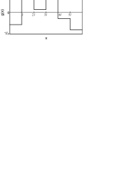
Figure 1: Sample path of a piecewise constant random force $g(x)$.

Assuming that the probability that $|g(x)|=g_{0}$ equals zero, i.e., the probability density $u(g)$ is not concentrated at the edges of the interval $[-g_{0},g_{0}]$, one can make sure that $I\to 1$ and so $\langle L\rangle\to\infty$ as $f\to g_{0}$. Hence, at $f=g_{0}$ the condition ${X_{t}|}_{t\to\infty}\to\infty$ holds almost surely, i.e., with probability one. In contrast, if the probability density $u(g)$ has unbounded support with $g_{0}=\infty$ as, e.g., for a Gaussian distribution, then $I<1$ and so $\langle L\rangle$ is finite for all finite values of the driving force $f$. In other words, in this case particles cannot be transported to an arbitrary large distance. It is therefore we consider here only a class of probability densities $u(g)$ with bounded support. It should be noted in this context that, since infinite values of $g(x)$ are physically not relevant, the assumption of bounded support is not too restrictive.

Our aim is to study the long-time behavior of the particle position $X_{t}$ at $f\geq g_{0}$. The main statistical characteristic of $X_{t}$ is its probability density function $P(x,t)$ defined as $P(x,t)=\langle\delta(x-X_{t})\rangle$, where $\delta(x)$ is the Dirac $\delta$ function. If the solution of Eq. (1) were known for all sample paths of $g(x)$, it would be, in principle, possible to determine $P(x,t)$ directly from the definition. However, this approach is difficult to implement and, what is more important, it is not necessary for finding the long-time behavior of the moments of $X_{t}$. Moreover, since at long times $X_{t}$ can be accurately evaluated as a total length of the intervals $(nl,nl+l)$ ($n=0,1,\ldots$) which a particle passes, many of the details of the particle dynamics described by Eq. (1) are needless for this purpose.

It is therefore reasonable to consider, instead of the model based on Eq. (1), the unidirectional CTRW of a particle on a semi-infinite one-dimensional lattice with the period $l$. Introduced more than four decades ago MW , the CTRW model has become one of the most effective and powerful tools in the theory of anomalous diffusion (see, e.g., Refs. MK ; Z ; KRS ). Within this model, we describe the particle position by a discrete variable $Y_{t}=lN(t)$, where $N(t)$ is the random number of jumps up to time $t$. In order to guarantee that the long-time behavior of $Y_{t}$ and $X_{t}$ are the same, we assume that for all $n$ the waiting time $\tau^{(n)}$, i.e., the time of occupation of the site $nl$, is equal to the time that a particle spends moving from the site $nl$ to the site $nl+l$. If the inertial effects can be neglected then Eq. (1) yields $\tau^{(n)}=\nu l/(f+g^{(n)})$, where $g^{(n)}=g(x)$ and $x$ belongs to the $n$th interval, i.e., $x\in[nl,nl+l)$. Since the random forces $g_{n}$ are statistically independent and distributed with the same probability density $u(g)$, the waiting times $\tau^{(n)}$ are also statistically independent variables whose probability density is given by

$$p(\tau)=\left\{\begin{array}[]{ll}\displaystyle\frac{\nu l}{\tau^{2}}\,u\!\left(\frac{\nu l}{\tau}-f\right),\quad\tau\in[\tau_{\rm{min}},\tau_{\rm{max}}]\\[12.0pt] 0,\quad\rm{otherwise}\end{array}\right.,$$ (3)

where

$$\tau_{\rm{min}}=\frac{\nu l}{f+g_{0}},\quad\tau_{\rm{max}}=\frac{\nu l}{f-g_{0}}.$$ (4)

It is important to emphasize that the inertial effects, at least in the underdamped regime characterized by the condition $\nu\tau_{\rm{min}}/\mu\gg 1$ (weakly underdamped regime), can also be incorporated into the CTRW framework. In order to illustrate this, let us first write the particle velocity $v^{(n)}(\Delta t)$ [$\Delta t\in(0,\tau^{(n)})$] on the $n$th ($n\geq 1$) interval. The straightforward integration of Eq. (1) yields

$$v^{(n)}(\Delta t)=\frac{f+g^{(n)}}{\nu}+\left(v^{(n)}_{-}-\frac{f+g^{(n)}}{\nu}\right)\!e^{-\kappa\Delta t},$$ (5)

where $\kappa=\nu/\mu$ and $v^{(n)}_{-}=v^{(n)}(0)$ is the particle velocity at the left end of the $n$th interval. Introducing also the particle velocity at the right end of this interval, $v^{(n)}_{+}=v^{(n)}(\tau^{(n)})$, from Eq. (5) we obtain

$$v^{(n)}_{+}=\frac{f+g^{(n)}}{\nu}+\left(v^{(n)}_{-}-\frac{f+g^{(n)}}{\nu}\right)\!e^{-\kappa\tau^{(n)}}.$$ (6)

Then, taking into account that $l=\int_{0}^{\tau^{(n)}}d(\Delta t)\,v^{(n)}(\Delta t)$, with the help of Eqs. (5) and (6) we find

$$l=\frac{f+g^{(n)}}{\nu}\,\tau^{(n)}-\frac{v^{(n)}_{+}-v^{(n)}_{-}}{\kappa}.$$ (7)

Since in the case under consideration $\kappa\tau^{(n)}\gg 1$, the exponential term in Eq. (6) can be neglected yielding $v^{(n)}_{+}=(f+g^{(n)})/\nu$. According to this approximation, the particle velocity at the end of the $n$th interval is determined by the random force on this interval. Therefore, using the continuity condition for the particle velocity, $v^{(n)}_{-}=v^{(n-1)}_{+}$, we obtain $v^{(n)}_{-}=(f+g^{(n-1)})/\nu$. Substituting these expressions for $v^{(n)}_{+}$ and $v^{(n)}_{-}$ into Eq. (7), we arrive to the following result:

$$\tau^{(n)}=\frac{\kappa\nu l+g^{(n)}-g^{(n-1)}}{\kappa(f+g^{(n)})}.$$ (8)

It shows that in the weakly underdamped regime the waiting time $\tau^{(n)}$ depends not only on the random force $g^{(n)}$, as in the overdamped case, but also on the random force $g^{(n-1)}$. Since these forces are statistically independent, the probability density of the waiting time can be written in the form

$$p(\tau)=\int_{-g_{0}}^{g_{0}}\int_{-g_{0}}^{g_{0}}dgdg^{\prime}u(g)u(g^{\prime})\,\delta\!\left(\tau-\frac{\kappa\nu l+g-g^{\prime}}{\kappa(f+g)}\right)$$ (9)

if $\tau\in[\tau_{\rm{min}},\tau_{\rm{max}}]$, otherwise it equals zero. It is not difficult to verify that in the overdamped case (when $\kappa=\infty$) Eq. (9) reduces to Eq. (3).

Next, we express the first two moments of the random variable $Y_{t}$ through the waiting time probability density $p(\tau)$. Since the moments of $N(t)$ are known from the CTRW theory (see, e.g., Ref. Hughes ), we reproduce here only the main results related to our situation. Introducing the probability $\mathcal{P}(n,t)$ that $N(t)=n$, we define the $k$th moment of the particle position $Y_{t}$ in the usual way:

$$\langle Y^{k}_{t}\rangle=l^{k}\sum_{n=1}^{\infty}n^{k}\mathcal{P}(n,t)$$ (10)

$(k=1,2,\ldots)$. Then, using the Laplace transform of a function $h(t)$, $h_{s}=\mathcal{L}\{h(t)\}=\int_{0}^{\infty}dt\,e^{-st}h(t)$ ($\rm{Re}\,s>0$), and taking into account that $\mathcal{P}(0,t)=\int_{t}^{\infty}d\tau\,p(\tau)$ and

$$\mathcal{P}(n,t)=\int_{0}^{t}d\tau\,p(\tau)\mathcal{P}(n-1,t-\tau)$$ (11)

($n\geq 1$), we obtain

$$\langle Y^{k}_{t}\rangle_{s}=l^{k}\frac{1-p_{s}}{s}\left(p_{s}\frac{d}{dp_{s}}\right)^{\!k}\frac{1}{1-p_{s}}.$$ (12)

Finally, applying to Eq. (12) the inverse Laplace transform defined as $h(t)=\mathcal{L}^{-1}\{h_{s}\}=(1/2\pi i)\int_{c-i\infty}^{c+i\infty}ds\,e^{st}h_{s}$ ($c$ is chosen to be larger than the real parts of all singularities of $h_{s}$), we find the first

$$\langle Y_{t}\rangle=l\,\mathcal{L}^{-1}\!\left\{\frac{p_{s}}{s(1-p_{s})}\right\}$$ (13)

and the second

$$\langle Y^{2}_{t}\rangle=l^{2}\mathcal{L}^{-1}\!\left\{\frac{p_{s}^{2}+p_{s}}{s(1-p_{s})^{2}}\right\}$$ (14)

moments of $Y_{t}$, which in turn determine the variance of the particle position:

$$\sigma^{2}(t)=\langle Y^{2}_{t}\rangle-\langle Y_{t}\rangle^{2}.$$ (15)

III CONDITIONS OF ANOMALOUS DIFFUSION

As it follows from the waiting time probability density (9), the $m$th moment of the waiting time, $\overline{\tau^{m}}=\int_{0}^{\infty}d\tau\,\tau^{m}p(\tau)$ $(m=1,2,\ldots)$, can be written in the form

$$\overline{\tau^{m}}=\int_{-g_{0}}^{g_{0}}\int_{-g_{0}}^{g_{0}}dgdg^{\prime}u(g)u(g^{\prime})\!\left(\frac{\kappa\nu l+g-g^{\prime}}{\kappa(f+g)}\right)^{\!m}\!.$$ (16)

Since the probability density $u(g)$ is normalized on the interval $[-g_{0},g_{0}]$, from Eq. (16) it follows that $\overline{\tau^{m}}\leq(\nu l+2g_{0}/\kappa)^{m}/(f-g_{0})^{m}$. Thus, if $f>g_{0}$ then all these moments are finite, and so in this case the classical central limit theorem for sums of a random number of random variables GK is applied to $Y_{t}$. This implies that $\sigma^{2}(t)\propto t$ as $t\to\infty$, i.e., at $f>g_{0}$ the biased diffusion of particles is normal, and the rescaled probability density $\mathcal{P}(\psi,t)=\sigma(t)P(\langle Y_{t}\rangle+\sigma(t)\psi,t)$ in the long-time limit tends to the probability density $\mathcal{P}(\psi,\infty)=(2\pi)^{-1/2}e^{-\psi^{2}/2}$ of the standard normal distribution.

It is clear from the above that the anomalous long-time behavior of the variance $\sigma^{2}(t)$ is expected at $\overline{\tau^{2}}=\infty$ when the mentioned central limit theorem becomes inapplicable. The condition $\overline{\tau^{2}}=\infty$ implies $f=g_{0}$ that, in accordance with (4), yields $\tau_{\rm{min}}=\nu l/2g_{0}$ and $\tau_{\rm{max}}=\infty$. Since the divergence of $\overline{\tau^{2}}$ occurs when $p(\tau)$ at $\tau\to\infty$ tends to zero slowly enough, next we assume that

$$p(\tau)\sim\frac{a}{\tau^{1+\alpha}}$$ (17)

$(\tau\to\infty)$ with $a>0$ and $\alpha\in(0,2]$. Thus, the biased diffusion in a randomly layered medium is expected to be anomalous if both conditions, $f=g_{0}$ and $\alpha\in(0,2]$, hold. The former guarantees that the waiting time $\tau$ can be arbitrarily large ($\tau_{\rm{max}}=\infty$), and so it is a necessary condition for anomalous diffusion. We note also that in this case one may expect that the rescaled probability density $\mathcal{P}(\psi,t)$ at $t\to\infty$ approaches the stable probability density, as the generalized central limit theorem Feller suggests.

The coefficient of proportionality $a$ and the exponent $\alpha$ are in general not independent and can be found from the asymptotic behavior of the probability density $u(g)$ in the vicinity of the point $g=-g_{0}$. Indeed, using the condition $\int_{-g_{0}}^{g_{0}}dg\,gu(g)=0$, which is a consequence of the symmetry property of $u(g)$, from Eq. (9) at $f=g_{0}$ we obtain

$$p(\tau)\sim\frac{\nu l}{\tau^{2}}\left[1-\frac{g_{0}}{\kappa\nu l}\!\left(1-\tau\frac{\partial}{\partial\tau}\right)\right]u\!\left(\frac{\nu l}{\tau}-g_{0}\right)$$ (18)

($\tau\to\infty,\kappa\to\infty$). Then, assuming that

$$u(g)\sim b\!\left(1+\frac{g}{g_{0}}\right)^{\!\beta-1}\!,$$ (19)

where $g\to-g_{0}$, $b>0$ and $\beta>0$, the asymptotic formula (18) takes the form

$$p(\tau)\sim bg_{0}\!\left(\frac{\nu l}{g_{0}}\right)^{\!\beta}\!\left(1-\frac{\beta g_{0}}{\kappa\nu l}\right)\!\frac{1}{\tau^{1+\beta}}.$$ (20)

Finally, comparing (20) with (17), we find $\alpha=\beta$ and

$$a=a_{\rm{od}}\!\left(1-\frac{\alpha g_{0}}{\kappa\nu l}\right)\!,$$ (21)

where $a_{\rm{od}}=bg_{0}(\nu l/g_{0})^{\alpha}$ is the parameter $a$ in the overdamped limit. According to these results, the particle mass decreases the parameter $a$ in comparison with the overdamped case but does not change the exponent $\alpha$.

An example of $u(g)$ having the asymptotic behavior (19) is the probability density

$$u(g)=\frac{\Gamma(\beta+1/2)}{g_{0}\sqrt{\pi}\,\Gamma(\beta)}\!\left(1-\frac{g^{2}}{g_{0}^{2}}\right)^{\!\beta-1}\!,$$ (22)

where $\Gamma(x)=\int_{0}^{\infty}dy\,y^{x-1}e^{-y}$ is the gamma function, which corresponds to the symmetric beta distribution. According to Eq. (22), this distribution is unimodal with the maximum at $g=0$ if $\beta>1$, bimodal with infinite maxima at $g=\pm g_{0}$ if $\beta<1$, and uniform if $\beta=1$. Determining the parameter $b$ directly from the density function (22), for this example we obtain

$$a_{\rm{od}}=\frac{\Gamma(\alpha+1/2)}{2\sqrt{\pi}\,\Gamma(\alpha)}\left(\frac{2\nu l}{g_{0}}\right)^{\!\alpha}.$$ (23)

IV LAWS OF ANOMALOUS DIFFUSION

IV.1 Long-time behavior of the inverse Laplace transform

From a formal point of view, the moments $\langle Y_{t}\rangle$ and $\langle Y^{2}_{t}\rangle$ completely determine the variance $\sigma^{2}(t)$. But the calculation of the inverse Laplace transforms in Eqs. (13) and (14) is a difficult technical problem because of the contour integration in the complex plane $s$. Fortunately, in the long-time limit this problem can be avoided. Such a possibility provides the celebrated Tauberian theorem for the Laplace transform Feller which is widely used in the theory of CTRW and its applications. According to this theorem, if $h(t)$ is ultimately monotone and

$$h_{s}=\mathcal{L}\{h(t)\}\sim L\!\left(\frac{1}{s}\right)\!\frac{1}{s^{\rho}}$$ (24)

($0<\rho<\infty$) as $s\to 0$ then

$$h(t)=\mathcal{L}^{-1}\{h_{s}\}\sim\frac{1}{\Gamma(\rho)}\,L(t)\,t^{\rho-1}$$ (25)

as $t\to\infty$, where $L(t)$ is a slowly varying function at infinity. The term ‘slowly varying’ means that $L(\lambda t)\sim L(t)$, i.e., $\lim_{t\to\infty}L(\lambda t)/L(t)=1$, for all $\lambda>0$. We note that, in contrast to Eqs. (13) and (14), the parameter $s$ in (24) is assumed to be a positive real number.

The Tauberian theorem in the above form permits to find only the leading terms of the asymptotic expansion of the moments $\langle Y_{t}\rangle$ and $\langle Y^{2}_{t}\rangle$ as $t\to\infty$. If $\lim_{t\to\infty}\langle Y_{t}\rangle^{2}/\langle Y^{2}_{t}\rangle\neq 1$ then, according to the definition (15), these terms completely determine also the leading term of the long-time expansion of $\sigma^{2}(t)$. However, if $\lim_{t\to\infty}\langle Y_{t}\rangle^{2}/\langle Y^{2}_{t}\rangle=1$ then for finding the leading term of $\sigma^{2}(t)$ at least the first two terms of each of the asymptotic expansions of $\langle Y_{t}\rangle$ and $\langle Y^{2}_{t}\rangle$ should be evaluated. Remarkably, these terms can also be determined from the Tauberian theorem if the Laplace transforms $\langle Y_{t}\rangle_{s}$ and $\langle Y^{2}_{t}\rangle_{s}$ at $s\to 0$ have the asymptotic form

$$h_{s}-\frac{q}{s^{\eta}}\sim L\!\left(\frac{1}{s}\right)\!\frac{1}{s^{\rho}}$$ (26)

with $\eta>\rho$. In this case, replacing $h_{s}$ by $h_{s}-q/s^{\eta}$ and using the exact result $\mathcal{L}^{-1}\{1/s^{\eta}\}=t^{\eta-1}/\Gamma(\eta)$ Erd , from (25) we obtain

$$h(t)-\frac{q}{\Gamma(\eta)}t^{\eta-1}\sim\frac{1}{\Gamma(\rho)}\,L(t)\,t^{\rho-1}.$$ (27)

It should be noted that $qt^{\eta-1}/\Gamma(\eta)$ and $L(t)t^{\rho-1}/\Gamma(\rho)$ actually represent the first two terms of the long-time expansion of $h(t)$ only if $\eta>\rho$. In the opposite case, when $L(1/s)/s^{\rho}$ is the leading term of the asymptotic expansion of $h_{s}$, this may not be true. The reason is that in this case the second term of the asymptotic expansion of $\mathcal{L}^{-1}\{L(1/s)/s^{\rho}\}$ at $t\to\infty$ may not be negligible in comparison with $qt^{\eta-1}/\Gamma(\eta)$. To illustrate this fact, let us assume that $L(1/s)=k\ln(1/s)$ ($k$ is a scale factor) and $\rho=2$, and consider the Laplace transform $h_{s}=q/s^{\eta}+(k/s^{2})\ln(1/s)$. Since $\mathcal{L}^{-1}\{(1/s^{2})\ln(1/s)\}=t(\ln t+\gamma-1)$, where $\gamma=0.5772$ is the Euler constant Erd , for the inverse Laplace transform of $h_{s}$ we obtain an exact result $h(t)=qt^{\eta-1}/\Gamma(\eta)+kt(\ln t+\gamma-1)$. If $\eta>2$ and $t\to\infty$ then, keeping in $h(t)$ the two leading terms, in accordance with (27) we find $h(t)-qt^{\eta-1}/\Gamma(\eta)\sim kt\ln t$. However, if $\eta\leq 2$ then the second term of the asymptotic expansion of $\mathcal{L}^{-1}\{L(1/s)/s^{\rho}\}$, $k(\gamma-1)t$, is not negligible compared to $qt^{\eta-1}/\Gamma(\eta)$ and, as a consequence, the asymptotic formula (27) does not hold. In this case only the leading term of $h(t)$, $kt\ln t$, is determined from the Tauberian theorem. Thus, while at $\eta>\rho$ the first two terms of the asymptotic expansion of $h(t)$ can be determined from the modified Tauberian theorem, Eqs. (26) and (27), to solve this problem in the opposite case it is necessary to go beyond the Tauberian theorem.

Next, we use the Tauberian theorem, Eqs. (24) and (25), and its modified version, Eqs. (26) and (27), to find the long-time behavior of the first two moments, $\langle Y_{t}\rangle$ and $\langle Y^{2}_{t}\rangle$, and the variance $\sigma^{2}(t)$ in the case of anomalous diffusion, i.e., when the conditions $f=g_{0}$ and $\alpha\in(0,2]$ hold simultaneously. Since the asymptotic solution of the CTRW is different for different intervals of $\alpha$ Shles , we consider the cases with $\alpha\in(0,1)$, $\alpha\in(1,2)$, $\alpha=1$, and $\alpha=2$ separately.

IV.2 $\alpha\in(0,1)$

In this case it is convenient to represent the Laplace transform of the waiting time probability density $p({\tau})$ in the form

$$p_{s}=1-\int_{\tau_{\rm{min}}}^{\infty}d\tau\,(1-e^{-s\tau})p(\tau),$$ (28)

which follows from the definition $p_{s}=\int_{\tau_{\rm{min}}}^{\infty}d\tau\,e^{-s\tau}p(\tau)$ and the normalization condition $\int_{\tau_{\rm{min}}}^{\infty}d\tau\,p(\tau)=1$. Introducing the new variable of integration $x=s\tau$ and using the asymptotic formula (17), we obtain

$$1-p_{s}\sim s^{\alpha}a\int_{0}^{\infty}dx\,\frac{1-e^{-x}}{x^{1+\alpha}}$$ (29)

as $s\to 0$. An integration by parts together with the integral representation of the gamma function AS , $\Gamma(x)=\int_{0}^{\infty}dy\,e^{-y}y^{x-1}$, reduces (29) to the form

$$1-p_{s}\sim\frac{a\Gamma(1-\alpha)}{\alpha}\,s^{\alpha}.$$ (30)

Now, using this result and the Laplace transforms

$$\langle Y_{t}\rangle_{s}=l\,\frac{p_{s}}{s(1-p_{s})},\quad\;\langle Y_{t}^{2}\rangle_{s}=l^{2}\frac{p_{s}^{2}+p_{s}}{s(1-p_{s})^{2}}$$ (31)

of the first two moments of $Y_{t}$, we find in the limit $s\to 0$:

$$\langle Y_{t}\rangle_{s}\sim\frac{l\alpha}{a\Gamma(1-\alpha)}\,\frac{1}{s^{1+\alpha}}$$ (32)

and

$$\langle Y_{t}^{2}\rangle_{s}\sim\frac{2l^{2}\alpha^{2}}{a^{2}\Gamma^{2}(1-\alpha)}\,\frac{1}{s^{1+2\alpha}}.$$ (33)

Since these asymptotic formulas are particular cases of the asymptotic formula (24) in which the slowly varying function $L(1/s)$ is a constant, from (25) we obtain in the long-time limit

$$\langle Y_{t}\rangle\sim\frac{l\alpha}{a\Gamma(1-\alpha)\Gamma(1+\alpha)}\,t^{\alpha}$$ (34)

and

$$\langle Y_{t}^{2}\rangle\sim\frac{2l^{2}\alpha^{2}}{a^{2}\Gamma^{2}(1-\alpha)\Gamma(1+2\alpha)}\,t^{2\alpha}.$$ (35)

Thus, in this case $\lim_{t\to\infty}\langle Y_{t}\rangle^{2}/\langle Y^{2}_{t}\rangle\neq 1$ and the above asymptotic expressions yield

$$\sigma^{2}(t)\sim\frac{l^{2}\alpha^{2}}{a^{2}\Gamma^{2}(1-\alpha)}\left(\!\frac{2}{\Gamma(1+2\alpha)}-\frac{1}{\Gamma^{2}(1+\alpha)}\right)\!t^{2\alpha}.$$ (36)

According to this result, which agrees with that obtained in the context of the asymptotic solution of the CTRW Shles , subdiffusion occurs if $\alpha\in(0,1/2)$ and superdiffusion if $\alpha\in(1/2,1)$. If $\alpha=1/2$ then $\sigma^{2}(t)\propto t$ and, in accordance with the commonly used terminology, the biased diffusion is normal. However, for normal diffusion processes both the mean and variance are proportional to time. Therefore, since $\langle Y_{t}\rangle\propto t^{1/2}$ at $\alpha=1/2$, this type of diffusion should be more appropriately termed as quasi-normal. It is also worthy to note that, according to Eqs. (21) and (36), the larger is the particle mass, the stronger is diffusion.

IV.3 $\alpha\in(1,2)$

Since in this case $\lim_{t\to\infty}\langle Y_{t}\rangle^{2}/\langle Y^{2}_{t}\rangle=1$ (see below), for finding the long-time behavior of $\sigma^{2}(t)$ we should determine the first two terms of the asymptotic expansion of $\langle Y_{t}\rangle$ and $\langle Y_{t}^{2}\rangle$ as $t\to\infty$. To this end, taking into account that at $\alpha\in(1,2)$ the mean waiting time $\overline{\tau}=\int_{\tau_{\rm{min}}}^{\infty}d\tau\,\tau p(\tau)$ exists, we use the following formula:

$$p_{s}=1-\overline{\tau}s-\int_{\tau_{\rm{min}}}^{\infty}d\tau(1-s\tau-e^{-s\tau})p(\tau).$$ (37)

Proceeding in the same way as before, we obtain

$$p_{s}-1+\overline{\tau}s\sim\frac{a\Gamma(2-\alpha)}{\alpha(\alpha-1)}\,s^{\alpha}$$ (38)

as $s\to 0$, and the straightforward calculation of the Laplace transforms (31) yields

$$\langle Y_{t}\rangle_{s}-\frac{l}{\overline{\tau}}\,\frac{1}{s^{2}}\sim\frac{la\Gamma(2-\alpha)}{\overline{\tau}^{2}\alpha(\alpha-1)}\,\frac{1}{s^{3-\alpha}}$$ (39)

and

$$\langle Y_{t}^{2}\rangle_{s}-\frac{2l^{2}}{\overline{\tau}^{2}}\,\frac{1}{s^{3}}\sim\frac{4l^{2}a\Gamma(2-\alpha)}{\overline{\tau}^{3}\alpha(\alpha-1)}\,\frac{1}{s^{4-\alpha}}.$$ (40)

These asymptotic formulas are particular cases of the asymptotic formula (26) with $L(1/s)=\rm{const}$. Therefore, using the well-known property of the gamma function, $\Gamma(1+x)=x\Gamma(x)$, from (27) we get

$$\langle Y_{t}\rangle-\frac{l}{\overline{\tau}}\,t\sim\frac{la}{\overline{\tau}^{2}\alpha(\alpha-1)(2-\alpha)}\,t^{2-\alpha}$$ (41)

and

$$\langle Y_{t}^{2}\rangle-\frac{l^{2}}{\overline{\tau}^{2}}\,t^{2}\sim\frac{4l^{2}a}{\overline{\tau}^{3}\alpha(\alpha-1)(2-\alpha)(3-\alpha)}\,t^{3-\alpha}$$ (42)

as $t\to\infty$. Accordingly, the long-time behavior of the variance $\sigma^{2}(t)$ is described by the power law

$$\sigma^{2}(t)\sim\frac{2l^{2}a}{\overline{\tau}^{3}\alpha(2-\alpha)(3-\alpha)}\,t^{3-\alpha}.$$ (43)

Thus, since $\alpha\in(1,2)$, the transport of particles is superdiffusive. Interestingly, depending on the exponent $\alpha$, the increase of the particle mass $\mu$ can either enhance or suppress the biased diffusion. In order to show this, we first use Eq. (16) with $m=1$ to represent the mean waiting time $\overline{\tau}$ in the form

$$\overline{\tau}=\overline{\tau}_{\rm{od}}\!\left(1+\frac{1}{\kappa\overline{\tau}_{\rm{od}}}-\frac{g_{0}}{\kappa\nu l}\right)\!,$$ (44)

where $\overline{\tau}_{\rm{od}}=\nu l\int_{-g_{0}}^{g_{0}}dg\,u(g)/(g_{0}+g)$ is the mean waiting time in the overdamped limit. Then, using this formula for $\overline{\tau}$, the expression (21) for the parameter $a$ and the condition $\kappa\tau_{\rm{min}}\gg 1$, we obtain

$$\frac{a}{\overline{\tau}^{3}}=\frac{a_{\rm{od}}}{\overline{\tau}_{\rm{od}}^{3}}\!\left(1-\frac{3}{\kappa\overline{\tau}_{\rm{od}}}+\frac{(3-\alpha)g_{0}}{\kappa\nu l}\right)\!.$$ (45)

According to this result, the biased diffusion is enhanced by the particle mass at $(3-\alpha)\overline{\tau}_{\rm{od}}>3\nu l/g_{0}$ and is suppressed at $(3-\alpha)\overline{\tau}_{\rm{od}}<3\nu l/g_{0}$. In particular, if the probability density $u(g)$ is given by Eq. (22) then

$$\overline{\tau}_{\rm{od}}=\frac{\nu l}{g_{0}}\,\frac{\alpha-1/2}{\alpha-1},$$ (46)

and so the former case occurs at $\alpha\in(1,3/2)$ and the latter at $\alpha\in(3/2,2)$.

IV.4 $\alpha=1$

Here our starting point is the Laplace transform of the waiting time probability density $p(\tau)$ represented as

$$p_{s}=1-aq_{s}-\int_{\tau_{\rm{min}}}^{\infty}d\tau(1-e^{-s\tau})\left(p(\tau)-\frac{a}{\tau^{2}}\right)\!,$$ (47)

where $q_{s}=\int_{\tau_{\rm{min}}}^{\infty}d\tau\,(1-e^{-s\tau})/\tau^{2}$. The advantage of this representation is that the term $aq_{s}$ accounts for the asymptotic behavior of $p(\tau)$, $p(\tau)\sim a/\tau^{2}$ as $\tau\to\infty$, in an explicit form. With the definition of the exponential integral AS , $E_{1}(x)=\int_{x}^{\infty}dy\,e^{-y}/y$, $q_{s}$ can be written as

$$q_{s}=s\frac{1-e^{-\xi}}{\xi}+sE_{1}(\xi)$$ (48)

($\xi=s\tau_{\rm{min}}$). Since $p(\tau)-a/\tau^{2}=o(1/\tau^{2})$ ($\tau\to\infty$), the integral term in Eq. (47) at $s\to 0$ can be neglected compared to $aq_{s}$. Therefore, taking into account the asymptotic formula $E_{1}(\xi)\sim\ln(1/s)$ AS , we obtain

$$1-p_{s}\sim as\ln\frac{1}{s}.$$ (49)

Using this result and Eq. (31) for calculating the leading terms of the Laplace transforms at $s\to 0$,

$$\langle Y_{t}\rangle_{s}\sim\frac{l}{a}\,\frac{1}{s^{2}\ln(1/s)},\quad\;\langle Y_{t}^{2}\rangle_{s}\sim\frac{l^{2}}{a^{2}}\,\frac{2}{s^{3}\ln^{2}(1/s)},$$ (50)

from the Tauberian theorem, Eqs. (24) and (25), we find the long-time behavior of the first two moments

$$\langle Y_{t}\rangle\sim\frac{l}{a}\,\frac{t}{\ln t},\quad\;\langle Y_{t}^{2}\rangle\sim\frac{l^{2}}{a^{2}}\,\frac{t^{2}}{\ln^{2}t}.$$ (51)

It should be noted that similar asymptotic formulas for $\langle Y_{t}\rangle$ and $\langle Y_{t}^{2}\rangle$ were obtained in Ref. Shles . But because of the use of the waiting time probability density $p(\tau)$ of a particular form, the asymptotic formulas derived in that paper do not depend on the parameter $a$. At the same time, as it was shown above, the parameter $a$ contains an important information about the role of quenched disorder and particle mass. In particular, Eq. (21) shows that the moments (51) increase with the particle mass.

Since $\lim_{t\to\infty}\langle Y_{t}\rangle^{2}/\langle Y_{t}^{2}\rangle=1$, for finding $\sigma^{2}(t)$ as $t\to\infty$ we need to know at least the two leading terms of the long-time expansion of $\langle Y_{t}\rangle$ and $\langle Y_{t}^{2}\rangle$. In principle, using Eq. (48) and the integral term in Eq. (47), we could easily find the asymptotic behavior of $1-p_{s}-as\ln(1/s)$ as $s\to 0$ and, in this way, obtain the second terms of the asymptotic expansion of $\langle Y_{t}\rangle_{s}$ and $\langle Y_{t}^{2}\rangle_{s}$. However, in contrast to the previous case, a straightforward application of the Tauberian theorem to this case does not provide a precise determination of the second terms of the asymptotic expansion of $\langle Y_{t}\rangle$ and $\langle Y_{t}^{2}\rangle$. As it was argued in Sec. IV.1, in order to find these terms it is necessary to go beyond the Tauberian theorem.

IV.5 $\alpha=2$

In this case we use the following representation for the Laplace transform of $p(\tau)$:

$$p_{s}=1-\overline{\tau}s-ar_{s}-\int_{\tau_{\rm{min}}}^{\infty}d\tau(1-s\tau-e^{-s\tau})\left(p(\tau)-\frac{a}{\tau^{3}}\right)\!,$$ (52)

where

$$r_{s} = \int_{\tau_{\rm{min}}}^{\infty}d\tau\,\frac{1}{\tau^{3}}(1-s\tau-e^{-s\tau})$$ (53)

$$= s^{2}\frac{1-2\xi-(1-\xi)\,e^{-\xi}}{2\xi^{2}}-\frac{s^{2}}{2}E_{1}(\xi).$$

This form of $p_{s}$ explicitly accounts for both the finiteness of $\overline{\tau}$ and the asymptotic behavior of $p(\tau)$. Since $p(\tau)-a/\tau^{3}=o(1/\tau^{3})$ ($\tau\to\infty$), at $s\to 0$ we can neglect the integral term in Eq. (52) in comparison with $ar_{s}$. This, together with the asymptotic formula $r_{s}\sim-(s^{2}/2)\ln(1/s)$ ($s\to 0$), yields

$$p_{s}-1+\overline{\tau}s\sim\frac{a}{2}s^{2}\ln\frac{1}{s}.$$ (54)

Using this result, the Laplace transforms of the first two moments of $Y_{t}$ at $s\to 0$ can be written as

$$\langle Y_{t}\rangle_{s}-\frac{l}{\overline{\tau}}\,\frac{1}{s^{2}}\sim\frac{la}{2\overline{\tau}^{2}}\,\frac{1}{s}\ln\frac{1}{s}$$ (55)

and

$$\langle Y_{t}^{2}\rangle_{s}-\frac{2l^{2}}{\overline{\tau}^{2}}\,\frac{1}{s^{3}}\sim\frac{2l^{2}a}{\overline{\tau}^{3}}\,\frac{1}{s^{2}}\ln\frac{1}{s}.$$ (56)

Therefore, in accordance with the modified Tauberian theorem, Eqs. (26) and (27), we obtain

$$\langle Y_{t}\rangle-\frac{l}{\overline{\tau}}\,t\sim\frac{la}{2\overline{\tau}^{2}}\,\ln t$$ (57)

and

$$\langle Y_{t}^{2}\rangle-\frac{l^{2}}{\overline{\tau}^{2}}\,t^{2}\sim\frac{2l^{2}a}{\overline{\tau}^{3}}\,t\ln t.$$ (58)

As a consequence, the long-time behavior of the variance is described by the asymptotic formula

$$\sigma^{2}(t)\sim\frac{l^{2}a}{\overline{\tau}^{3}}\,t\ln t.$$ (59)

The fact that $\sigma^{2}(t)$ increases faster than $t$ is in accordance with the asymptotic formula (43). Indeed, while $t^{3-\alpha}$ approaches $t$, the coefficient of proportionality between $\sigma^{2}(t)$ and $t$ tends to infinity as $\alpha\to 2-0$. We note also that the ratio $a/\overline{\tau}^{3}$ at $\alpha=2$ is determined by the same Eq. (45). Therefore, if $u(g)$ is given by Eq. (22) then the larger is the particle mass, the weaker is diffusion.

In conclusion of this subsection we would like to draw attention to the differences between our model and one-dimensional iterated maps which generate trajectories according to the rule $x_{n+1}=x_{n}+F(x_{n})$. It is usually assumed DetMap that $F(x)$ is an antisymmetric, $F(-x)=-F(x)$, and periodic, $F(x+N)=F(x)$ ($N$ is an integer), function. Due to these conditions, there is no drift, i.e., the quantity $\langle x\rangle\equiv\langle x_{n+t}-x_{n}\rangle$ can be taken to be zero, where the angular brackets denote an average over a properly chosen set of initial conditions of $x_{n}$ and $t$ plays the role of the number of iterations. The same property, $\langle x\rangle=0$, holds also for maps perturbed by time dependent noise BMWG and quenched disorder Rad with zero means. Thus, these maps are unbiased and so the variance of $x_{n+t}-x_{n}$, i.e., $\langle x^{2}\rangle-\langle x\rangle^{2}$, reduces to $\langle x^{2}\rangle$. Using the CTRW theory, in most cases it is possible to write this variance as the inverse Laplace transform and use the ordinary Tauberian theorem for finding its long-time behavior DetMap ; BMWG . In contrast, in our model $\langle Y_{t}\rangle$ grows with time and although the moments $\langle Y_{t}\rangle$ and $\langle Y_{t}^{2}\rangle$ can also be represented as the inverse Laplace transform, the variance $\sigma^{2}(t)=\langle Y_{t}^{2}\rangle-\langle Y_{t}\rangle^{2}$ cannot. Therefore, if $\lim_{t\to\infty}\langle Y_{t}\rangle^{2}/\langle Y_{t}^{2}\rangle=1$, the leading term of the asymptotic expansion of $\sigma^{2}(t)$ as $t\to\infty$ cannot be determined by applying the ordinary Tauberian theorem. We have solved this problem (for $\alpha\neq 1$) by using the modified Tauberian theorem. It should also be noted that adding to $F(x)$ a weak uniform bias breaks the symmetry of the system and, as a consequence, leads to a time dependence of $\langle x\rangle$ BiasMap . However, the biased maps considered in BiasMap do not exhibit anomalous diffusion at long times.

IV.6 Role of thermal fluctuations

We complete our analysis with a qualitative discussion of the role of thermal fluctuations. These fluctuations can be accounted for by adding the thermal noise term to the right-hand side of Eq. (1). In this case some important conclusions can be drawn from the asymptotic behavior of the correlator $K(x,y)=\langle[U(x)-U(y)]^{2}\rangle$ as $|x-y|\to\infty$, where $U(x)$ is the random potential that corresponds to the random force $g(x)=-dU(x)/dx$. Since under thermal fluctuations particles can move in both directions, the random force and potential should be determined on the entire $x$-axis. Using the properties of $g(x)$ and the continuity condition for $U(x)$ with $U(0)=0$, we obtain

$$U(x)=-(x-nl)g^{(n)}+U(nl).$$ (60)

Here, $x\in[nl,nl+l)$, $n=0,\pm 1,\ldots$, and $U(nl)=-l\sum_{s=0}^{n}g^{(s)}+lg^{(n)}$ if $n\geq 0$ and $U(nl)=l\sum_{s=-1}^{n}g^{(s)}$ if $n\leq-1$. Taking into account that the random forces $g^{(s)}$ with different $s$ are statistically independent, the definition of the correlator $K(x,y)$ and Eq. (60) lead to the asymptotic expression

$$K(x,y)\sim l\sigma^{2}_{g}|x-y|$$ (61)

($|x-y|\to\infty$), where $\sigma^{2}_{g}=\int_{-g_{0}}^{g_{0}}dg\,g^{2}u(g)$.

The systems with $K(x,y)\propto|x-y|$ have long been a subject of extensive study (see, e.g., Refs. BG ; Mon and references therein). A remarkable result obtained for these systems in the overdamped regime is that there always exists a threshold value $f_{\rm{tr}}$ of the external force $f$ in which the depinning transition occurs. This transition is characterized by vanishing the average particle velocity in the pinning state, when $f\leq f_{\rm{tr}}$, while in the depinning state, when $f>f_{\rm{tr}}$, particles move with a nonzero average velocity which strongly depends on $f$. According to Den , if $g(x)$ is a bounded function then $f_{\rm{tr}}<g_{0}$ ($f_{\rm{tr}}\to g_{0}$ as the temperature approaches zero) and the mean first-passage time in the depinning and pinning states is finite and infinite, respectively. Since the moments of the first-passage time can be associated with the moments of the waiting time, we may expect therefore that at nonzero temperatures and $f<g_{0}$ the exponent $\alpha$ and so the character of anomalous diffusion becomes depending on $f$ (the diffusion behavior at $f>g_{0}$ is expected to be normal). Specifically, with decreasing of $f$ from $g_{0}$ to $f_{\rm{tr}}$ the exponent $\alpha$ should also decrease from 2 to 1, and if $f<f_{\rm{tr}}$ then $\alpha<1$. Of course, in order to find the dependence of $\alpha$ on $f$ and the diffusion laws a quantitative consideration of the problem is needed. It is especially important because the effects arising from the joint action of quenched disorder and thermal fluctuations are often unexpected and even counterintuitive.

V CONCLUSIONS

We have studied in the long-time limit the unidirectional transport of particles which occurs under a constant force in a randomly layered medium. The influence of the layers is modeled by a piecewise constant random force whose values in different layers are assumed to be independent and identically distributed with bounded support. We have reduced the problem of the unidirectional transport, initially formulated in the framework of the motion equation, to a continuous-time random walk on a semi-infinite chain. The main statistical characteristic of this approach, the waiting time probability density, is expressed through the probability density of the random force and particle characteristics, including the particle mass. By analyzing the dependence of the moments of the waiting time on the external force, we have formulated the conditions under which the biased diffusion exhibits the anomalous behavior. It has been shown that this behavior may occur only if the external force is equal to the boundary value of the random force.

In order to find in the anomalous regime the long-time behavior of the first and second moments of the particle position, we have used the Tauberian theorem and its modified version allowing, in most cases, to determine the first two terms of the asymptotic expansion of these moments. Within this approach, we have found, with one exception, the explicit asymptotic formulas for the variance of the particle position, i.e., the laws of diffusion. The time dependence of the variance is completely controlled by the exponent describing the asymptotic behavior of the probability density of the random force in the vicinity of its minimum value. It has also been shown that, depending on the value of this exponent, the particle mass in the weakly underdamped regime can either enhance or suppress the anomalous diffusion without changing its time dependence.

References

- (1) L. F. Richardson, Proc. Roy. Soc. London A 110, 709 (1926).
- (2) H. Scher and E. W. Montroll, Phys. Rev. B 12, 2455 (1975).
- (3) T. H. Solomon, E. R. Weeks, and H. L. Swinney, Phys. Rev. Lett. 71, 3975 (1993).
- (4) H. Yang, G. Luo, P. Karnchanaphanurach, T.-M. Louie, I. Rech, S. Cova, L. Xun, and X. S. Xie, Science 302, 262 (2003).
- (5) P. Brault, C. Josserand, J.-M. Bauchire, A. Caillard, C. Charles, and R. W. Boswell, Phys. Rev. Lett. 102, 045901 (2009).
- (6) J. P. Bouchaud and A. Georges, Phys. Rep. 195, 127 (1990).
- (7) D. ben-Avraham and S. Havlin, Diffusion and Reactions in Fractals and Disordered Systems (Cambridge University Press, Cambridge, 2000).
- (8) R. Metzler and J. Klafter, Phys. Rep. 339, 1 (2000).
- (9) G. Zaslavsky, Phys. Rep. 371, 461 (2002).
- (10) Anomalous Transport: Foundations and Applications, edited by R. Klages, G. Radons, and I. M. Sokolov (Wiley-VCH, Berlin, 2008).
- (11) S. Scheidl, Z. Phys. B 97, 345 (1995); P. Le Doussal and V. M. Vinokur, Physica C 254, 63 (1995); P. E. Parris, M. Kuś, D. H. Dunlap, and V. M. Kenkre, Phys. Rev. E 56, 5295 (1997); D. A. Gorokhov and G. Blatter, Phys. Rev. B 58, 213 (1998); A. V. Lopatin and V. M. Vinokur, Phys. Rev. Lett. 86, 1817 (2001); P. Reimann and R. Eichhorn, ibid. 101, 180601 (2008).
- (12) M. N. Popescu, C. M. Arizmendi, A. L. Salas-Brito, and F. Family, Phys. Rev. Lett. 85, 3321 (2000); L. Gao, X. Luo, S. Zhu, and B. Hu, Phys. Rev. E 67, 062104 (2003); D. G. Zarlenga, H. A. Larrondo, C. M. Arizmendi, and F. Family, ibid. 75, 051101 (2007); S. I. Denisov, T. V. Lyutyy, E. S. Denisova, P. Hänggi, and H. Kantz, ibid. 79, 051102 (2009).
- (13) H. Kunz, R. Livi, and A. Sütő, Phys. Rev. E 67, 011102 (2003).
- (14) S. I. Denisov, M. Kostur, E. S. Denisova, and P. Hänggi, Phys. Rev. E 75, 061123 (2007); ibid. 76, 031101 (2007).
- (15) E. W. Montroll and G. H. Weiss, J. Math. Phys. 6, 167 (1965).
- (16) B. D. Hughes, Random Walks and Random Environments (Clarendon Press, Oxford, 1995), Vol. 1.
- (17) B. V. Gnedenko and V. Yu. Korolev, Random Summation: Limit Theorems and Applications (CRC Press, Boca Raton, 1996).
- (18) W. Feller, An Introduction to Probability Theory and its Applications (Wiley, New York, 1971), Vol. 2.
- (19) A. Erdélyi, Tables of Integral Transforms (McGraw-Hill, New York, 1954), Vol. 1.
- (20) M. F. Shlesinger, J. Stat. Phys. 10, 421 (1974).
- (21) M. Abramowitz and I. A. Stegun, Handbook of Mathematical Functions (Dover, New York, 1972).
- (22) T. Geisel and S. Thomae, Phys. Rev. Lett. 52, 1936 (1984); G. Zumofen and J. Klafter, Phys. Rev. E 47, 851 (1993); J. Dräger and J. Klafter, Phys. Rev. Lett. 84, 5998 (2000).
- (23) R. Bettin, R. Mannella, B. J. West, and P. Grigolini, Phys. Rev. E 51, 212 (1995).
- (24) G. Radons, Phys. Rev. Lett. 77, 4748 (1996).
- (25) E. Barkai and J. Klafter, Phys. Rev. Lett. 79, 2245 (1997); Phys. Rev. E 57, 5237 (1998).
- (26) C. Monthus, Lett. Math. Phys. 78, 207 (2006).
- (27) S. I. Denisov and R. Yu. Lopatkin, Phys. Scr. 56, 423 (1997); S. I. Denisov and W. Horsthemke, Phys. Rev. E 62, 3311 (2000).