Parametrized Abel–Jacobi maps
and abelian cycles in the Torelli group

Abstract

Let $\mathcal{I}_{g,\ast}$ denote the Torelli group of the genus $g\geq 2$ surface $S_{g}$ with one marked point. This is the group of homotopy classes (rel basepoint) of homeomorphisms of $S_{g}$ fixing the basepoint and acting trivially on $H\mathrel{\mathop{:}}\mkern-1.2mu=H_{1}(S_{g},\mathbb{Q})$. In 1983 Johnson constructed a beautiful family of invariants

$$\tau_{i}\colon H_{i}(\mathcal{I}_{g,\ast},\mathbb{Q})\to\textstyle{\bigwedge}^{i+2}H$$

for $0\leq i\leq 2g-2$, using a kind of Abel–Jacobi map for families. He used these invariants to detect nontrivial cycles in $\mathcal{I}_{g,\ast}$. Johnson proved that $\tau_{1}$ is an isomorphism, and asked if the same is true for $\tau_{i}$ with $i>1$.

The goal of this paper is to introduce various methods for computing $\tau_{i}$; in particular we prove that $\tau_{i}$ is not injective for any $2\leq i<g$, answering Johnson’s question in the negative. We also show that $\tau_{2}$ is surjective. For $g\geq 3$, we find many classes in the image of $\tau_{i}$ and use them to deduce that $H_{i}(\mathcal{I}_{g,\ast},\mathbb{Q})\neq 0$ for each $1\leq i<g$. This is in contrast with the case of mapping class groups. Many of our classes are stable, so we can deduce that $H_{i}(\mathcal{I}_{\infty,1},\mathbb{Q})$ is infinite-dimensional for each $i\geq 1$. Finally, we conjecture a new kind of “representation-theoretic stability” for the homology of the Torelli group, for which our results provide evidence.

1 Introduction

Let $S_{g}$ be a connected, closed, oriented surface of genus $g\geq 2$, let $H\mathrel{\mathop{:}}\mkern-1.2mu=H_{1}(S_{g},\mathbb{Q})$, and let $H_{\mathbb{Z}}\mathrel{\mathop{:}}\mkern-1.2mu=H_{1}(S_{g},\mathbb{Z})$. The (pointed) Torelli group $\mathcal{I}_{g,\ast}$ is the group of pointed homotopy classes of pointed homeomorphisms of $S_{g}$ acting trivially on $H_{\mathbb{Z}}$. Understanding $\mathcal{I}_{g,\ast}$, and particularly its (co)homology, is an important problem in topology and algebraic geometry (see, e.g., [Jo83], [Ha95] and [Mo99] for discussions).

Parametrized Abel–Jacobi maps. In [Jo83], Johnson produced a beautiful family of invariants, and used them to prove that certain cycles in $H_{\ast}(\mathcal{I}_{g,\ast},\mathbb{Q})$ are nontrivial. He did this by constructing, for each $0\leq i\leq 2g-2$, an $\operatorname{Sp}(2g,\mathbb{Z})$–equivariant homomorphism

$$\tau_{i}\colon H_{i}(\mathcal{I}_{g,\ast},\mathbb{Q})\to\textstyle{\bigwedge}^{i+2}H.$$

The maps $\tau_{i}$ can be described using a kind of parametrized Abel–Jacobi map, as follows. We first outline an explicit construction of $\tau_{1}\colon H_{1}(\mathcal{I}_{g,\ast},\mathbb{Q})\to\textstyle{\bigwedge}^{3}H$. Let $S_{g,\ast}$ denote $S_{g}$ with a marked point. For any $f\in\mathcal{I}_{g,\ast}$, the image $\tau_{1}([f])\in\textstyle{\bigwedge}^{3}H$ can be computed as follows. Construct the mapping torus

$$M_{f}\mathrel{\mathop{:}}\mkern-1.2mu=S_{g,\ast}\times[0,1]/(f(p),0)\sim(p,1).$$

This 3–manifold is naturally a bundle with section $S_{g,\ast}\to M_{f}\to S^{1}$, and the fact that $f$ acts trivially on $H_{1}(S_{g,\ast})$ implies that $H_{1}(M_{f})$ is canonically isomorphic to $H_{1}(S_{g,\ast})\times H_{1}(S^{1})$.

The Jacobian of a Riemann surface $S_{g}$ is the complex torus $\operatorname{Jac}(S_{g})\approx T^{2g}$given by $(H^{1}(S_{g},\mathbb{C}))^{*}/H_{1}(S_{g},\mathbb{Z})$. The Abel–Jacobi map is a holomorphic map$j\colon(S_{g},\ast)\to(\operatorname{Jac}(S_{g}),0)$ unique in its homotopy class, with the property that the induced map on fundamental group $j_{*}\colon\pi_{1}(S_{g},\ast)\to\pi_{1}(\operatorname{Jac}(S_{g,\ast}),0)\approx H_{\mathbb{Z}}$ is the abelianization. The composition

$$\pi_{1}(M_{f})\to H_{1}(M_{f})\approx H_{1}(S_{g,\ast})\times H_{1}(S^{1})\to H_{1}(S_{g,\ast})$$

induces a map

$$J\colon M_{f}\to\operatorname{Jac}(S_{g})$$ (1)

unique up to homotopy. Now $\tau_{1}([f])$ is defined as the image of the fundamental class $[M_{f}]\in H_{3}(M_{f},\mathbb{Q})$ under the induced map $J_{*}\colon H_{3}(M_{f},\mathbb{Q})\to H_{3}(\operatorname{Jac}(S_{g}),\mathbb{Q})\approx\textstyle{\bigwedge}^{3}H$.

For the definition of $\tau_{i}$ for all $i\geq 1$, let $\operatorname{{\cal T}}_{g,\ast}$ denote the Torelli space of Riemann surfaces diffeomorphic to $S_{g}$ endowed with a homology marking and a marked point; that is, $\operatorname{{\cal T}}_{g,\ast}$ is the quotient of the Teichmüller space $\operatorname{Teich}_{g,\ast}$ by the (free) action of $\mathcal{I}_{g,\ast}$. As $\operatorname{Teich}_{g,\ast}$ is contractible, we have that $H_{i}(\mathcal{I}_{g,\ast})\approx H_{i}(\operatorname{{\cal T}}_{g,\ast})$. Let

$$S_{g,\ast}\to\operatorname{{\cal T}}^{\ast}_{g,\ast}\overset{\pi}{\to}\operatorname{{\cal T}}_{g,\ast}$$ (2)

denote the universal $S_{g,\ast}$–bundle over $\operatorname{{\cal T}}_{g,\ast}$. There is also a universal bundle

$$\operatorname{Jac}(S_{g})\to\operatorname{{\cal T}}^{\operatorname{Jac}}_{g,\ast}\to\operatorname{{\cal T}}_{g,\ast}$$ (3)

of Jacobians, and the Abel–Jacobi map $j$ globalizes to give a (holomorphic) map

$$J\colon\operatorname{{\cal T}}^{*}_{g,\ast}\to\operatorname{{\cal T}}^{\operatorname{Jac}}_{g,\ast}.$$ (4)

Note that the zero element in each fiber gives a section of the bundle (3), and that $\mathcal{I}_{g,*}$ acts trivially on the fiber $\operatorname{Jac}(S_{g})$. These are the only obstructions to triviality for a torus bundle, so the bundle $\operatorname{{\cal T}}^{\operatorname{Jac}}_{g,\ast}\to\operatorname{{\cal T}}_{g,\ast}$ is topologically trivial. Let $p\colon\operatorname{{\cal T}}^{\operatorname{Jac}}_{g,\ast}\to\operatorname{Jac}(S_{g})$ denote projection to the torus factor.

We can now define $\tau_{i}(\sigma)$ for an $i$–cycle $\sigma$ in $\operatorname{{\cal T}}_{g,\ast}$, where $i\leq 2g-2$. The inverse image $\pi^{-1}(\sigma)$ in $\operatorname{{\cal T}}^{\ast}_{g,\ast}$ gives an $(i+2)$–cycle (this operation is sometimes called the Gysin homomorphism), and we can take the image of this $(i+2)$–cycle under the composition $p\circ J$, giving us an element $\tau_{i}(\sigma)\in H_{i+2}(\operatorname{Jac}(S_{g}),\mathbb{Q})\approx\textstyle{\bigwedge}^{i+2}H$.

The images of the maps $\tau_{0}$ and $\tau_{1}$ are worked out explicitly in Section 2 below. In particular, as proved by Hain in [Ha97] (see also Proposition 2.2 below), the map $\tau_{1}$ agrees with the original, purely algebraic definition of the Johnson homomorphism, which plays a central role in the study of $\mathcal{I}_{g,\ast}$. In a series of papers, Johnson proved that $\tau_{1}$ is, modulo torsion, an isomorphism (see [Jo83] for a summary of this work). In his 1983 paper [Jo83], Johnson constructed $\tau_{i}$ as above, and as Question C he asked if $\tau_{i}$ is a rational isomorphism for all $i\geq 1$. In [Ha97] Hain used continuous cohomology and representation theory to prove that $\tau_{2}$ is not injective; it seems that Hain’s method cannot be extended to the case when $i\geq 3$. In this paper we develop a method for concretely computing the values of the $\tau_{i}$. Our first main result answers Johnson’s question negatively in degrees $2\leq i<g$.

Theorem 1.1.

The map $\tau_{i}$ is not injective for any $2\leq i<g$.

Remark. The map $\tau_{i}$ can be defined on integral homology, with target $\textstyle{\bigwedge}^{i+2}H_{\mathbb{Z}}$. Since the target is free abelian, and since the elements we construct in the kernel of $\tau_{i}$ are integral classes, Theorem 1.1 implies that our classes also lie in the kernel of this integral version of $\tau_{i}$.

We will find a number of sources for nontrivial cycles in $\ker\tau_{i}$. One source will be certain “abelian cycles” coming from bounding pair maps (see below). These cycles are determined by certain collections of simple closed curves. The (non)vanishing of $\tau_{i}$ on such cycles will depend on the topological configuration of the collection of curves, namely whether or not they are “truly nested” (see Definition 3.3). The nontriviality of cycles in the kernel of $\tau_{i}$ is detected by combining certain operations in the homology of Torelli groups with other $\tau_{j}$ for $j\neq i$. We remark that Bestvina–Bux–Margalit [BBM] found nontrivial elements of $H_{3g-3}(\mathcal{I}_{g,\ast},\mathbb{Q})$; there is no $\tau_{i}$ defined in this dimension since $3g-3>2g-2$.

In the positive direction of Johnson’s question, we show that the $\tau_{i}$ detect nontrivial classes in each dimension; in particular we prove that $\tau_{2}$ is surjective. Our general theorem in this direction is most simply stated in the language of symplectic representation theory. From the standard exact sequence

$$1\to\mathcal{I}_{g,\ast}\to\operatorname{Mod}_{g,\ast}\to\operatorname{Sp}(2g,\mathbb{Z})\to 1,$$

the conjugation action of $\operatorname{Mod}_{g,\ast}$ on $\mathcal{I}_{g,\ast}$ descends to an action of $\operatorname{Sp}(2g,\mathbb{Z})$ by outer automorphisms, which gives $H_{i}(\mathcal{I}_{g,1},\mathbb{Q})$ the structure of an $\operatorname{Sp}(2g,\mathbb{Z})$–module. The construction of the homomorphism $\tau_{i}$ shows that it is $\operatorname{Sp}(2g,\mathbb{Z})$–equivariant.

Irreducibility remark. Let $V$ be an irreducible $\operatorname{Sp}(2g,\mathbb{Q})$–representation. It follows from Proposition 3.2 of [Bo] that $V$ is an irreducible $\operatorname{Sp}(2g,\mathbb{Z})$–module (this is close to the statement of the Borel Density Theorem in this case). Henceforth we will not make the distinction of irreducibility over $\mathbb{Q}$ versus irreducibility over $\mathbb{Z}$.

The algebraic irreducible representations of $\operatorname{Sp}(2g,\mathbb{Q})$ are classified by their highest weight vectors (a good reference is [FH]). Choose a set $\lambda_{1},\ldots,\lambda_{g}$ of fundamental weights for $\operatorname{Sp}(2g,\mathbb{Q})$. A highest weight vector is a linear combination $\lambda=\sum c_{i}\lambda_{i}$, where the coefficients are nonnegative integers. We denote the irreducible representation of $\operatorname{Sp}(2g,\mathbb{Q})$ with highest weight vector $\lambda$ by $V(\lambda)$. For example, $V(\lambda_{i})$ is the kernel of the contraction $C_{i}:\textstyle{\bigwedge}^{i}H\to\textstyle{\bigwedge}^{i-2}H$ defined by:

$$C_{i}(x_{1}\wedge\cdots\wedge x_{i})=\sum_{j<k}(-1)^{j+k+1}\omega(x_{j},x_{k})x_{1}\wedge\cdots\wedge\widehat{x}_{j}\wedge\cdots\wedge\widehat{x}_{k}\wedge\cdots\wedge x_{i}$$ (5)

The $\operatorname{Sp}(2g,\mathbb{Q})$–module $\textstyle{\bigwedge}^{k}H$ for $k\leq g$ decomposes into irreducible representations as

$$\textstyle{\bigwedge}^{k}H\approx V(\lambda_{k})\oplus V(\lambda_{k-2})\oplus\cdots\oplus V(\lambda_{\varepsilon})$$

where $\varepsilon=0$ or $1$ depending on whether $k$ is even or odd. Our second main result is the following.

Theorem 1.2.

Suppose $g\geq 2$. Then for $1\leq i\leq g-2$, we have

$$\tau_{i}(H_{i}(\mathcal{I}_{g,\ast},\mathbb{Q}))\supseteq V(\lambda_{i+2})\oplus V(\lambda_{i}).$$ (6)

In addition, for $1\leq i\leq g$ and $i$ even, we have

$$\tau_{i}(H_{i}(\mathcal{I}_{g,\ast},\mathbb{Q}))\supseteq V(\lambda_{i-2}).$$ (7)

For $i=g-1$, the term $V(\lambda_{i+2})$ in (6) is not meaningful, but the proof of Theorem 1.2 will show that $\tau_{g-1}(H_{g-1}(\mathcal{I}_{g,\ast},\mathbb{Q}))$ contains $V(\lambda_{g-1})$.

Since $\textstyle{\bigwedge}^{4}H=V(\lambda_{4})\oplus V(\lambda_{2})\oplus V(\lambda_{0})$, we have the following.

Corollary 1.3.

Let $g\geq 2$. Then $\tau_{2}$ is surjective.

We wish to point out that Morita announced in [Mo89] that a map closely related to $\tau_{2}$ is surjective. As another corollary of Theorem 1.2 we deduce the following.

Corollary 1.4.

Let $g\geq 2$. Then $H_{i}(\mathcal{I}_{g,*},\mathbb{Q})$ is nonzero for each $1\leq i<g$. When $g$ is even, $H_{g}(\mathcal{I}_{g,*},\mathbb{Q})$ is also nonzero.

Theorem 1.2 also provides evidence for a “homological stability” conjecture for the Torelli group, which we now outline.

Stable classes. The nontrivial classes we construct above are stable. In order to explain this we need to extend our picture to surfaces with boundary. Let $\mathcal{I}_{g,1}$ denote the group of homotopy classes of homeomorphisms of the compact genus $g\geq 2$ surface $S_{g,1}$ with one boundary component, acting trivially on $H_{1}(S_{g,1},\mathbb{Z})$. Here both the homeomorphisms and homotopies are taken to be the identity on $\partial S_{g,1}$.

The map $S_{g,1}\to S_{g,*}$ that identifies $\partial S_{g,1}$ to a single (marked) point gives a homomorphism $\nu\colon\mathcal{I}_{g,1}\to\mathcal{I}_{g,\ast}$ whose kernel is the cyclic group generated by the Dehn twist about $\partial S_{g,1}$. We define a homomorphism

$$\widehat{\tau_{i}}\colon H_{i}(\mathcal{I}_{g,1},\mathbb{Q})\to\textstyle{\bigwedge}^{i+2}H$$

by composing $\tau_{i}$ with the map on homology induced by $\nu$. From the proof of Theorem 1.2, we immediately obtain, for $1\leq i\leq g-2$, that

$$\widehat{\tau_{i}}(H_{i}(\mathcal{I}_{g,1},\mathbb{Q}))\supseteq V(\lambda_{i+2})\oplus V(\lambda_{i}).$$

Now, the natural inclusion $S_{g,1}\hookrightarrow S_{g+1,1}$ induces a natural inclusion $\mathcal{I}_{g,1}\hookrightarrow\mathcal{I}_{g+1,1}$. We can thus form the direct limit

$$\mathcal{I}_{\infty,1}\mathrel{\mathop{:}}\mkern-1.2mu=\lim_{g\rightarrow\infty}\mathcal{I}_{g,1},$$

called the stable Torelli group. It is easy to see from the definitions that the following diagram is commutative, where $H_{g}=H_{1}(S_{g,1},\mathbb{Q})$ and $H_{g+1}=H_{1}(S_{g+1,1},\mathbb{Q})$:

It follows that each nontrivial class in $H_{i}(\mathcal{I}_{g,1},\mathbb{Q})$ constructed above is stable, in that its image in $H_{i}(\mathcal{I}_{g+k,1},\mathbb{Q})$ is nontrivial for each $k\geq 0$. As homology preserves direct limits, and since $\dim V(\lambda_{i})\to\infty$ as $g\to\infty$, we have the following corollary.

Corollary 1.5.

For each $i\geq 1$, the vector space $H_{i}(\mathcal{I}_{\infty,1},\mathbb{Q})$ is infinite-dimensional.

This greatly contrasts with the situation for the stable mapping class group, whose odd-dimensional homology vanishes, and whose even-dimensional homology has finite rank (see [MW]).

A stability conjecture for $H_{\ast}(\mathcal{I}_{g,1},\mathbb{Q})$. The stability of the homology classes we construct, together with the presence of nontrivial $\operatorname{Sp}(2g,\mathbb{Z})$–modules in $H_{i}(\mathcal{I}_{g,1},\mathbb{Q})$, shows that the classical kind of homological stability, satisfied for example by $\operatorname{GL}_{n},\operatorname{Out}(F_{n})$, and the mapping class group, does not hold for the Torelli group. However, our results provide evidence for a new kind of “representation-theoretic stability”, which we now describe.

We begin with the simplest, quickest-to-state form of our conjecture. When we want to emphasize the group that acts, we will denote by $V(\lambda)_{2g}$ the irreducible $\operatorname{Sp}(2g,\mathbb{Z})$–representation with highest weight vector $\lambda$.

Conjecture 1.6 (Representation stability, I).

The homology of the Torelli group is representation stable with respect to $g$: for each $i\geq 1$ and each $g$ sufficiently large (depending on $i$), we have that the $\operatorname{Sp}(2g,\mathbb{Z})$–module $H_{i}(\mathcal{I}_{g,1},\mathbb{Q})$ contains the representation $V(\lambda)_{2g}$ with some multiplicity $0\leq m\leq\infty$ if and only if for each $h\geq g$ the $\operatorname{Sp}(2h,\mathbb{Z})$–module $H_{i}(\mathcal{I}_{h,1},\mathbb{Q})$ contains the representation $V(\lambda)_{2h}$ with multiplicity $m$, and similarly for $\mathcal{I}_{g,\ast}$ and $\mathcal{I}_{g}$.

Applying a result of Kawazumi–Morita [KM, Theorem 5.5], it can be deduced that the truth of this conjecture for $\mathcal{I}_{g,\ast}$ is equivalent to the truth of the conjecture for $\mathcal{I}_{g}$. We expect that the conjecture for $\mathcal{I}_{g,1}$ is similarly equivalent.

Morita has conjectured [Mo99, Conjecture 3.4] that the $\operatorname{Sp}$–invariant stable cohomology of $\mathcal{I}_{g,1}$ is generated by the even Miller–Morita–Mumford classes. Morita’s Conjecture would immediately imply the special case of Conjecture 1.6 when $V(\lambda)$ is the trivial representation.

We would like to refine Conjecture 1.6 by giving a more direct comparison of the homology of different Torelli groups. Of course we cannot ask for an isomorphism of $H_{i}(\mathcal{I}_{g,1},\mathbb{Q})$ and $H_{i}(\mathcal{I}_{h,1},\mathbb{Q})$ as modules since the first is an $\operatorname{Sp}(2g,\mathbb{Z})$–module and the second is an $\operatorname{Sp}(2h,\mathbb{Z})$–module. However, there are meaningful injectivity and surjectivity statements one can ask for, as we will see in Conjecture 1.7 below.

Our main conjecture makes predictions about the finite-dimensional part of $H_{i}(\mathcal{I}_{g,1},\mathbb{Q})$. We define the finite-dimensional homology $H_{i}(\mathcal{I}_{g,1},\mathbb{Q})^{\operatorname{fd}}$ to be the subspace of $H_{i}(\mathcal{I}_{g,1},\mathbb{Q})$ consisting of those vectors whose $\operatorname{Sp}(2g,\mathbb{Z})$–orbit spans a finite-dimensional vector space.

Conjecture 1.7 (Representation stability, II).

For each $i\geq 1$ and each $g$ sufficiently large (depending on $i$), the following hold:

Finite-dimensionality: The natural map $i_{\ast}\colon H_{i}(\mathcal{I}_{g,1},\mathbb{Q})^{\operatorname{fd}}\to H_{i}(\mathcal{I}_{g+1,1},\mathbb{Q})$ induced by the inclusion $i\colon\mathcal{I}_{g,1}\to\mathcal{I}_{g+1,1}$ has image contained in $H_{i}(\mathcal{I}_{g+1,1},\mathbb{Q})^{\operatorname{fd}}$.

Injectivity: The natural map $i_{\ast}\colon H_{i}(\mathcal{I}_{g,1},\mathbb{Q})^{\operatorname{fd}}\to H_{i}(\mathcal{I}_{g+1,1},\mathbb{Q})$ is injective.

Surjectivity: The span of the $\operatorname{Sp}(2g+2,\mathbb{Z})$–orbit of $i_{\ast}(H_{i}(\mathcal{I}_{g,1},\mathbb{Q})^{\operatorname{fd}})$ equals all of $H_{i}(\mathcal{I}_{g+1},\mathbb{Q})^{\operatorname{fd}}$.

Rationality: Every irreducible $\operatorname{Sp}(2g,\mathbb{Z})$–subrepresentation in $H_{i}(\mathcal{I}_{g,1},\mathbb{Q})^{\operatorname{fd}}$ is the restriction of an irreducible $\operatorname{Sp}(2g,\mathbb{Q})$–representation.

Type preserving: For any representation $V(\lambda)_{2g}\subset H_{i}(\mathcal{I}_{g,1},\mathbb{Q})^{\operatorname{fd}}$, the span of the $\operatorname{Sp}(2g+2,\mathbb{Z})$–orbit of $V(\lambda)_{2g}$ is isomorphic to $V(\lambda)_{2g+2}$.

Remarks.

1. A form of the Margulis Superrigidity Theorem (see [Ma], Theorem VIII.B) gives that any finite-dimensional representation (over $\mathbb{C}$) of $\operatorname{Sp}(2g,\mathbb{Z})$ either (virtually) extends to a (rational) representation of $\operatorname{Sp}(2g,\mathbb{R})$ or factors through a finite group. The “rationality” statement of Conjecture 1.7 is meant to rule out the latter possibility for subrepresentations of $H_{i}(\mathcal{I}_{g,1},\mathbb{Q})^{\operatorname{fd}}$.

2. It is possible to embed the $\operatorname{Sp}(2g,\mathbb{Q})$–module $V(\lambda_{i})_{2g}$ into the $\operatorname{Sp}(2g+2,\mathbb{Q})$–module $V(\lambda_{i+1})_{2g+2}$ so that the $\operatorname{Sp}(2g+2,\mathbb{Q})$–span of the image is all of $V(\lambda_{i+1})_{2g+2}$, and similarly for other pairs of irreducible representations. The “type preserving” statement in Conjecture 1.7 is meant to rule out this type of phenomenon.

3. Theorem 1.2 shows that the “stable range” in Conjecture 1.7, meaning the smallest $g$ for which $H_{i}(\mathcal{I}_{g,1},\mathbb{Q})^{\operatorname{fd}}$ stabilizes, must be at least $i$.

4. Mess [Me] proved that $H_{1}(\mathcal{I}_{2,1},\mathbb{Q})$ contains an infinite-dimensional, irreducible permutation $\operatorname{Sp}(4,\mathbb{Z})$–module. Similarly, the classes in $H_{3g-2}(\mathcal{I}_{g,1},\mathbb{Q})$ found by Bestvina–Bux–Margalit [BBM] span an infinite-dimensional, permutation $\operatorname{Sp}(2g,\mathbb{Z})$–module. Neither of these is “stable” in $g$; one might hope that stably, such representations do not arise, and all irreducible $\operatorname{Sp}$–submodules of $H_{i}(\mathcal{I}_{g,1},\mathbb{Q})$ are finite-dimensional for $g\gg i$.

5. Conjecture 1.6 and Conjecture 1.7 would give an affirmative answer to Question 7.9 of Hain–Looijenga [HL], which asked “Is $H^{k}(T_{g})$ expressible as an $\operatorname{Sp}_{2g}(\mathbb{Z})$–module in a way that is independent of $g$ if $g$ is large enough?”

Evidence. As mentioned above, Theorem 1.2 provides evidence in every dimension for Conjectures 1.6 and 1.7. Both conjectures are true in dimension 1, by Johnson’s computation that $H_{1}(\mathcal{I}_{g,1})\approx H_{1}(\mathcal{I}_{g,\ast})\approx V(\lambda_{3})\oplus V(\lambda_{1})$ and $H_{1}(\mathcal{I}_{g})\approx V(\lambda_{3})$. Other than this, very little is known about the homology of the Torelli group. However, in low dimensions we have work of Hain, who found a large subspace of $H_{2}(\mathcal{I}_{g})$, and Sakasai, who found a large subspace of $H_{3}(\mathcal{I}_{g})$. We describe their methods and state their results in Section 5.3; the resulting subspaces satisfy Conjecture 1.7.

Since this paper was first distributed, Boldsen–Dollerup [BD] have proved that the surjectivity condition in Conjecture 1.7 holds for $H_{2}(\mathcal{I}_{g,1};\mathbb{Q})$ as long as $g\geq 6$.

In the paper [CF] we situate these conjectures in the much broader framework of a general theory of “representation stability”.

Outline of paper. In §2 we outline our general approach to computing the $\tau_{i}$, and explicitly work out $\tau_{0}$ and $\tau_{1}$ as a warmup. In §3 we give two ways of computing $\tau_{i}$. We first show how to compute the image under $\tau_{i}$ of the “product” of a cycle supported on a subsurface with a bounding pair map. We then give a vanishing result for cycles built from gluing subsurfaces along a pair-of-pants. We then apply these tools in order to compute both vanishing and nonvanishing results for $\tau_{i}$ of abelian cycles in $H_{i}(\mathcal{I}_{g,\ast})$. Section 4 gives a computation of $\tau_{i}$ on cycles in $H_{i}(\mathcal{I}_{g,\ast})$ that are surface bundles over certain tori in $H_{i-2}(\mathcal{I}_{g})$. This computation reveals the phenomenon of an even/odd dichotomy for the nonvanishing/vanishing of cycles; in particular we obtain many new nonzero classes in $H_{i}(\mathcal{I}_{g,\ast})$. In §5 we use all the computations above to complete the proofs of Theorem 1.1 and Theorem 1.2. We conclude by explaining how theorems of Hain and Sakasai give further evidence for Conjecture 1.6 and Conjecture 1.7.

Acknowledgements. We are extremely grateful to the referee for all of their comments and corrections.

2 Setup and first examples

In this section, we outline the framework of the computations in this paper. We then compute $\tau_{0}$ and $\tau_{1}$ as the simplest examples of our methods. For the rest of the paper, all homology groups are taken with coefficients in $\mathbb{Q}$, although the reader may just as well imagine the coefficients are $\mathbb{Z}$ if preferred.

Bundles representing homology classes. As mentioned in the introduction, the bundle $S_{g,\ast}\to\operatorname{{\cal T}}^{\ast}_{g,\ast}\overset{\pi}{\to}\operatorname{{\cal T}}_{g,\ast}$ described in (2) is the universal genus $g$ surface bundle equipped with a section and a trivialization of its fiberwise homology. (All the surface bundles we consider in this paper will be endowed with such a trivialization, namely an identification of the homology of each fiber with $H_{1}(S_{g})$.) This means that for any base $B$, there is a bijective correspondence between such bundles over $B$ up to isomorphism and maps $f\colon B\to\operatorname{{\cal T}}_{g,\ast}$ up to homotopy; the correspondence is induced by pulling back the universal bundle along the map $f$.

Given a homology class $\sigma\in H_{i}(\operatorname{{\cal T}}_{g,\ast})$, we say that a bundle $S_{g,\ast}\to E\to B$ and a homology class $x\in H_{i}(B)$ represent $\sigma$ if the induced homology class $f_{*}(x)\in H_{i}(\operatorname{{\cal T}}_{g,\ast})$ is equal to $\sigma$. It is sometimes mentally simplifying to assume that $B$ is a closed manifold, which can be done as follows. Thom [Th, Theorem II.29] proved that every homology class in a closed orientable manifold has an integral multiple which can be represented by (the fundamental class of) a closed submanifold. This can be strengthened to show that every homology class in any CW complex has an odd integral multiple which can be represented by a closed submanifold, see e.g. Conner [Co, Corollary 15.3]. Thus every homology class $\sigma\in H_{i}(\operatorname{{\cal T}}_{g,\ast})$ has a multiple represented by the fundamental class $[B]\in H_{i}(B)$ for a bundle $S_{g,\ast}\to E^{i+2}\to B^{i}$ of closed manifolds. Although this assumption is not logically necessary for our arguments, we let it influence us by often referring to the representing homology class as $[B]\in H_{i}(B)$.

Parametrized Abel–Jacobi maps. Given a bundle $S_{g,\ast}\to E\to B$ and homology class $[B]\in H_{i}(B)$ representing $\sigma\in H_{i}(\operatorname{{\cal T}}_{g,\ast})\approx H_{i}(\mathcal{I}_{g,\ast})$, we can use the bundle $E\to B$ to compute the Johnson invariant $\tau_{i}(\sigma)$, as follows. The globalized Abel–Jacobi map (4) restricts to a map $J_{E}\colon E\to T^{2g}$ defined up to homotopy. We remark that the target should be thought out of not just as a torus $T^{2g}$, but as a $K(H_{\mathbb{Z}},1)$, so that choosing a basis for $H_{\mathbb{Z}}$ gives corresponding coordinates on $T^{2g}$.

We call the map $J_{E}\colon E\to T^{2g}$ a parametrized Abel–Jacobi map, since on each fiber it restricts to a map homotopic to the classical Abel–Jacobi map. Since $T^{2g}$ is aspherical, it is determined (up to homotopy) by the induced map on fundamental group, which is determined by the following two properties:

1. On the fiber $S_{g}$ the map $J_{E}$ induces the abelianization $\pi_{1}(S_{g})\to H_{\mathbb{Z}}$.

2. On the image of the section $B\to E$ the map $J_{E}$ is constant.

In this situation, the preimage of $[B]$ in $E$ is a class $[E]\in H_{i+2}(E)$. Then the Johnson invariant $\tau_{i}$ can be computed as follows:

$$\tau_{i}(\sigma)=(J_{E})_{*}[E]\in H_{i+2}(T^{2g})\approx\textstyle{\bigwedge}^{i+2}H$$ (8)

The key to our computations in this paper is to find convenient models for $E\to B$ and for the parametrized Abel–Jacobi map $J_{E}$ so that $(J_{E})_{*}[E]$ can be calculated explicitly.

Computing $\tau_{0}$. The intersection form on $H=H_{1}(S)$ can be represented by an element $\omega\in\textstyle{\bigwedge}^{2}H$; if $a_{1},b_{1},\ldots,a_{g},b_{g}$ is a symplectic basis, we have

$$\omega=a_{1}\wedge b_{1}+\cdots+a_{g}\wedge b_{g}.$$

Since $\tau_{0}$ is a map from $H_{0}(\mathcal{I}_{g,\ast})\approx\mathbb{Q}$, it is determined by the image of the generator.

Proposition 2.1.

The image of the generator under $\tau_{0}\colon H_{0}(\mathcal{I}_{g,\ast})\to\textstyle{\bigwedge}^{2}H$ is $\omega$.

Proof.

Since the generator of $H_{0}(\mathcal{I}_{g,\ast})$ is induced by the inclusion of a point, we see that the image of $\tau_{0}$ is equal to $j_{\ast}[\Sigma_{g}]\in H_{2}(T^{2g})=\textstyle{\bigwedge}^{2}H$, the image of the fundamental class $[\Sigma_{g}]$ under the Abel–Jacobi map, which we now compute.

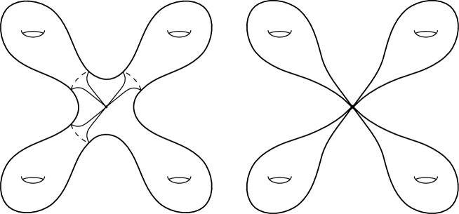
Figure 1: The surface $S_{g}$ and its quotient $Y=\bigvee T_{i}$.

We begin by giving an explicit construction of a map $j$ homotopic to the Abel–Jacobi map that will be useful for our purposes. We will sometimes refer to such a map $j$ as an Abel–Jacobi map, since it is uniquely defined only up to homotopy. First, let $Y=\bigvee_{i=1}^{g}T_{i}$ be the wedge of 2–dimensional tori. There is a natural quotient map $S_{g}\to Y$, obtained for example by collapsing a graph as in Figure 1. In any torus, specifying $k$ distinct coordinates determines a $k$–dimensional subspace homeomorphic to a torus $T^{k}$. The coordinates of $T^{2g}$ are labeled by the symplectic basis $a_{1},b_{1},\ldots,a_{g},b_{g}$. Identify the $i$th torus $T_{i}$ with the torus $T^{2}\subset T^{2g}$ determined by the $a_{i}$ and $b_{i}$ coordinates. These identifications agree at the origins of the tori $T_{i}$, and thus induce an inclusion $Y=\bigvee T_{i}\hookrightarrow T^{2g}$. The composition $j\colon S_{g}\to Y\to T^{2g}$ is homotopic to the Abel–Jacobi map; to see this, it is enough to observe that the generators $a_{i}$ and $b_{i}$ of $\pi_{1}(S_{g})$ are taken to the corresponding elements of $\pi_{1}(T^{2g})=H_{\mathbb{Z}}$.

Finally, we must find $j_{*}[S_{g}]\in H_{2}(T^{2g})$. Under the quotient map $S_{g}\to Y=\bigvee T_{i}$, the fundamental class $[S_{g}]\in H_{2}(S_{g})$ is sent to $\sum[T_{i}]\in H_{2}(Y)$. Then $T_{i}$ is included as the torus determined by the $a_{i}$ and $b_{i}$ coordinates; under the natural isomorphism $H_{k}(T^{2g})\approx\textstyle{\bigwedge}^{k}H$, this torus represents $a_{i}\wedge b_{i}$. Thus we have

$$j_{\ast}\colon[S_{g}]\mapsto\sum[T_{i}]\mapsto\sum a_{i}\wedge b_{i}=\omega$$

as claimed. ∎

Computing $\tau_{1}$. In [Jo80], Johnson used the action of $\mathcal{I}_{g,\ast}$ on the second universal $2$–step nilpotent quotient of $\pi_{1}(S_{g,\ast})$ to define in a purely algebraic way an $\operatorname{Sp}(2g,\mathbb{Z})$–equivariant homomorphism $\tau_{J}:\mathcal{I}_{g,\ast}\to\textstyle{\bigwedge}^{3}H$ which is now called the Johnson homomorphism.

Recall that a bounding pair map in $\mathcal{I}_{g,\ast}$ is a composition of two Dehn twists $T_{\alpha}T_{\beta}^{-1}$, where $\alpha$ and $\beta$ are nonhomotopic, homologous, disjoint nonseparating simple closed curves. For any bounding pair map, up to homeomorphism of $S_{g}$, the curves $\alpha$ and $\beta$ are of the form depicted in Figure 2a. Let $S^{\prime}$ be the component of $S_{g}\setminus(\alpha\cup\beta)$ not containing the basepoint, and fix $1<k\leq g$ so that $S^{\prime}$ has genus $k-1$. Let $\{a_{1},b_{1},\ldots,a_{g},b_{g}\}$ be a symplectic basis for $H_{1}(S_{g})$ with the property that $\alpha$ (oriented with $S^{\prime}$ on the left) is homologous to $a_{k}$, and so that $\{a_{1},b_{1},\ldots,a_{k-1},b_{k-1},a_{k}\}$ descends to a basis for $H_{1}(S^{\prime})$. Johnson showed in [Jo80] that

$$\tau_{J}(f)=(a_{1}\wedge b_{1}+\cdots+a_{k-1}\wedge b_{k-1})\wedge a_{k}.$$ (9)

The following proposition was stated by Johnson in [Jo83] as the motivation for investigating the maps $\tau_{i}$. Hain gave a proof in [Ha97] using the work of Sullivan and the cup product structure on the cohomology of mapping tori. Our proof is elementary, and more importantly, it can be generalized to higher-dimensional cycles. Indeed, the ideas introduced in this proof will appear throughout Sections 3 and 4.

Proposition 2.2 (Johnson, Hain [Ha97]).

The map $\tau_{1}\colon H_{1}(\mathcal{I}_{g,*})\to\textstyle{\bigwedge}^{3}H$ coincides with the Johnson homomorphism $\tau_{J}$.

Proposition 2.2 can be thought of as a “parametrized” version of the proof of Proposition 2.1 above.

Proof.

Building on work of Birman [Bi] and Powell [Po], Johnson proved in [Jo79] that $\mathcal{I}_{g,*}$ is generated by bounding pair maps for $g\geq 3$; see Hatcher–Margalit [HM] for a modern proof. (For $g=2$ separating twists are also necessary; however $\tau_{J}$ is known to vanish on separating twists, and $\tau_{1}$ vanishes on separating twists by Proposition 3.6.) Thus it suffices to check that $\tau_{1}$ coincides on bounding pair maps with Johnson’s map $\tau_{J}$.

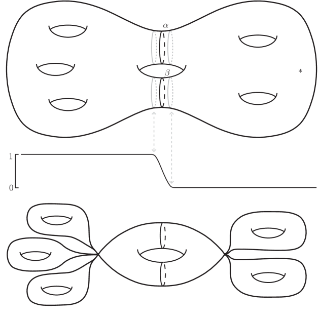
Figure 2: a. The surface $S_{g,*}$ and the bounding pair $f$. b. The $a_{k}$ component of $\delta$.
c. The quotient $Y=\bigcup T_{i}$. The torus $T_{k}$ is in the middle, the tori $T_{i}$ for $i<k$ are on the left, and the tori $T_{i}$ for $i>k$ are on the right.

To compute $\tau_{1}(f)$, we first find a bundle $S_{g,*}\to E\to S^{1}$ representing $[f]\in H_{1}(\mathcal{I}_{g,*})$. The natural choice is the mapping torus $S_{g,*}\to M_{f}\to S^{1}$, which can be defined as the quotient

$$M_{f}=S_{g}\times[0,1]/(f(p),0)\sim(p,1).$$

The image of the basepoint $\ast\in S_{g}$ in each fiber gives a section of this bundle.

To describe the parametrized Abel–Jacobi map $J=J_{M_{f}}\colon M_{f}\to T^{2g}$, we will define $J$ on the cylinder $S_{g}\times[0,1]$ in such a way that it descends to $M_{f}=S_{g}\times[0,1]/\sim$. One obvious first approach is to define $J$ on the fiber $S_{g}\times\{0\}$ just by the Abel–Jacobi map $j$. The identification $\sim$ then forces the restriction of $J$ to $S_{g}\times\{1\}$ to be $j\circ f$. We might naively try to define $J$ simply by interpolating between $j$ and $j\circ f$:

$$J(p,t)\overset{?}{=}(1-t)\cdot j(p)+t\cdot j\circ f(p)$$ (10)

But $j$ and $j\circ f$ take values in the torus $T^{2g}$, so the first term $(1-t)\cdot j(p)$, for example, is not well-defined. However, we can accomplish this idea as follows. Since $f\in\mathcal{I}_{g,\ast}$, the two maps $j\circ f$ and $j$ induce the same map on the fundamental group and thus are homotopic. Equivalently, their pointwise difference $j\circ f-j$ is homotopically trivial as a map $S_{g}\to T^{2g}$. We may thus take a lift $\delta\colon S_{g}\to\mathbb{R}^{2g}$ of $j\circ f-j$; that is, the unique map satisfying $\delta(\ast)=0$ and

$$j\circ f-j=\delta\bmod{\mathbb{Z}^{2g}}.$$

For convenience, we will take $j$ to be an Abel–Jacobi map chosen so that the only coordinate of $\delta$ which is nonzero is that corresponding to $a_{k}$, and in that coordinate $\delta$ is of the form shown in Figure 2b. In particular $\delta(p)$ only depends on the “horizontal” coordinate of $p$ in the depiction in Figure 2a.

One way to ensure this is as follows. The twists $T_{\alpha}$ and $T_{\beta}$ are supported on annular neighborhoods $N_{\alpha}$ and $N_{\beta}$ of $\alpha$ and $\beta$ respectively. Identify these with $S^{1}\times[0,1]$ so that $T_{\alpha}(\theta,t)=(\theta+t,t)$ on $N_{\alpha}$ and $T_{\beta}^{-1}(\theta,t)=(\theta-t,t)$ on $N_{\beta}$. We define $j$ to be zero on $S_{g}\setminus(N_{\alpha}\cup N_{\beta})$; on $N_{\alpha}$ and on $N_{\beta}$ the $a_{k}$ coordinate of $j$ is given by $\theta$, and all other coordinates are zero. Since $j=j\circ f$ outside $N_{\alpha}\cup N_{\beta}$, the function $\delta$ is constant there. On $N_{\alpha}$ the $a_{k}$ coordinate of $j\circ f-j$ is given by $t$, and similarly on $N_{\beta}$ by $-t$. Thus $\delta$ has the properties claimed above.

Now we may define $J\colon M_{f}\to T^{2g}$ by

$$J(p,t)=j(p)+t\cdot\delta(p).$$

Substituting $j\circ f-j=\delta\bmod{\mathbb{Z}^{2g}}$, we see that this definition realizes the idea set out in (10) above. The bounding pair map $f$ does not factor through a wedge of tori, but it does factor through the space $Y=\bigcup T_{i}$ depicted in Figure 2c, which is the union of tori $T_{i}$ meeting pairwise in at most 1 point. We may assume that the sympletic basis $\{a_{1},b_{1},\ldots,a_{g},b_{g}\}$ was chosen so that $\{a_{i},b_{i}\}$ descends to a basis for $H_{1}(T_{i})$ for each $1\leq i\leq g$. It is easy to see that $j$ factors through $S_{g}\to Y$ as well, and thus so does $\delta$. From our explicit formula for $J$, we see that $J$ factors through the space

$$Z\mathrel{\mathop{:}}\mkern-1.2mu=Y\times[0,1]/(f(p),0)\sim(p,1),$$

which fibers as a bundle $Y\to Z\to S^{1}$. Just as $Y$ is the union of tori, we see that $Z$ is the union of torus bundles $T_{i}\to Z_{i}\to S^{1}$ meeting pairwise in at most a circle.The quotient $M_{f}\to Z$ maps the fundamental class $[M_{f}]$ to $\sum[Z_{i}]$. Thus it remains to understand $J_{*}[Z_{i}]$.

Note that $f$ is supported on the torus $T_{k}$; it follows that for $i\neq k$ the torus bundle $T_{i}\to Z_{i}\to S^{1}$ is in fact a product $Z_{i}\approx T_{i}\times S^{1}$. For $i\neq k$, since $j$ and $j\circ f$ agree on $T_{i}$, we have that $\delta$ is constant on $T_{i}$. Since $\delta$ is as depicted in Figure 2b, we have that the $a_{k}$ component of $\delta$ is 1 on $T_{i}$ for $i<k$ and is 0 on $T_{i}$ for $i>k$. Thus when $i<k$, the restriction of $J$ to $Z_{i}\approx T_{i}\times S^{1}$ is given by

$$J(p,t)=j(p)+(0,\ldots,0,t,0,\ldots,0).$$

This is just the inclusion of $T^{3}\subset T^{2g}$ determined by the $a_{i}$, $b_{i}$, and $a_{k}$ coordinates; in particular, we have

$$J_{*}[Z_{i}]=a_{i}\wedge b_{i}\wedge a_{k}\mbox{\ for \ }i<k.$$

When $i>k$, we have that $J(p,t)=j(p)$, so the image of $J$ is contained in the 2–dimensional subspace determined by $a_{i}$ and $b_{i}$. Since $H_{3}(T^{2})\subset H_{3}(T^{2g})$ is trivial, we have $J_{*}[Z_{i}]=0$ for $i>k$. Finally, on $T_{k}$ the function $\delta$ is nonconstant; however, the images of both $j$ and $\delta$ are contained in the 2–dimensional subspace determined by $a_{k}$ and $b_{k}$. The same is thus true of the image of $J$, so $J_{*}[Z_{k}]=0$ as well. We conclude that

$$J_{*}\colon[M_{f}]\mapsto\sum_{i=1}^{g}[Z_{i}]\mapsto\sum_{i<k}a_{i}\wedge b_{i}\wedge a_{k}=\tau_{J}(f),$$

as desired. ∎

Andy Putman has pointed out that one can view the idea of this proof as “moving the cycle represented by $M_{f}$ to the boundary of Torelli space”, where the computation is easier to verify; from this viewpoint, moving to the boundary of Torelli space corresponds to the degeneration of $S_{g}$ to the union-of-tori $Y=\bigcup T_{i}$.

3 Tools for computing $\tau_{i}$

In this section we provide two of our main tools for computing $\tau_{i}$, and we use them to compute $\tau_{i}$ on abelian cycles. It will be convenient for us to state our results for the case of surfaces with boundary, namely for the map $\widehat{\tau_{i}}$ mentioned in the introduction. For simplicity of notation we will call this map $\tau_{i}$ as well.

Product with a bounding pair map. Our first proposition gives a method to bootstrap up homology classes which can be detected using $\tau_{i}$. Let $S_{g,1}\hookrightarrow S_{g+1,1}$ be the standard inclusion, inducing an inclusion $\mathcal{I}_{g,1}\hookrightarrow\mathcal{I}_{g+1,1}$. Let $f=T_{\alpha}T_{\beta}^{-1}$ be a bounding pair map supported in the complement of $S_{g,1}$, and let $a$ be the common homology class of $\alpha$ and $\beta$ (oriented with $S_{g,1}$ on the left). Then we have a natural map

$$\cdot\times f\colon H_{i}(\mathcal{I}_{g,1})\to H_{i+1}(\mathcal{I}_{g+1,1})$$

given by the Gysin homomorphism $H_{i}(\mathcal{I}_{g,1})\to H_{i+1}(\mathcal{I}_{g,1}\times\langle f\rangle)$ followed by the inclusion $\mathcal{I}_{g,1}\times\langle f\rangle\to\mathcal{I}_{g+1,1}$.

Proposition 3.1.

Let $f$ be as above. For any $\sigma\in H_{i}(\mathcal{I}_{g,1})$ we have

$$\tau_{i+1}(\sigma\times f)=\tau_{i}(\sigma)\wedge a.$$

Note that Proposition 2.2 can be deduced from Proposition 2.1 by applying Proposition 3.1.

Proof.

Let $S_{g,1}\to E^{\prime}\to B$ be a bundle with a homology class $[B]\in H_{i}(B)$ representing $\sigma\in H_{i}(\mathcal{I}_{g,1})$. There is an associated bundle $S_{g,*}\to E\to B$ representing $\sigma\in H_{i}(\mathcal{I}_{g,*})$. Recall that by (8), $\tau_{i}(\sigma)$ is the image of $[E]$ under the parametrized Abel–Jacobi map $J_{E}\colon E\to T^{2g}$.

Similarly, there is a bundle $S_{g+1,*}\to\overline{E}\to B\times S^{1}$ representing

$$[B]\times[S^{1}]\mapsto\sigma\times f\in H_{i+1}(\mathcal{I}_{g+1,*}).$$

Here $[B]\times[S^{1}]\in H_{i+1}(B\times S^{1})$ is the class corresponding to $[B]\otimes[S^{1}]\in H_{i}(B)\otimes H_{1}(S^{1})$ under the Künneth formula; the preimage of $[B]\times[S^{1}]$ is a class denoted $[\overline{E}]\in H_{i+3}(\overline{E})$.

To compute $\tau_{i+1}(\sigma\times f)$, we need to explicitly describe the space $\overline{E}$. By $S_{1,1,*}$ we mean a surface of genus 1 with one boundary component and a separate marked point. We can glue $E^{\prime}$ to the trivial bundle $S_{1,1,*}\times B$ fiberwise along their common boundary component $S^{1}\times B$. Now let

$$\overline{E}=(E^{\prime}\cup(S_{1,1,*}\times B))\times[0,1]/\sim,$$

where the identification is given by:

$$(e,0) \sim(e,1) \text{ for }e \in E^{\prime}$$

$$\big{(}(f(p),b),0\big{)} \sim\big{(}(p,b),1\big{)} \text{ for }(p,b) \in S_{1,1,*}\times B$$

Note that $\overline{E}$ naturally has the structure of a bundle

$$S_{g+1,*}\to\overline{E}\to B\times S^{1}.$$

Over $B\subset B\times S^{1}$, this bundle restricts to

$$S_{g+1,*}\to E^{\prime}\cup(S_{1,1,*}\times B)\to B,$$

which represents $[B]\mapsto\iota(\sigma)\in H_{i}(\mathcal{I}_{g+1,*})$. Over $S^{1}\subset B\times S^{1}$, it restricts to the mapping torus $S_{g+1,*}\to M_{f}\to S^{1}$ of $f$, which represents $[S^{1}]\mapsto[f]\in H_{1}(\mathcal{I}_{g+1,*})$. It follows that $\overline{E}\to B\times S^{1}$ represents $[B]\times[S^{1}]\mapsto\sigma\times f\in H_{i+1}(\mathcal{I}_{g+1,*})$, as desired.

Now we construct the parametrized Abel–Jacobi map $J_{\overline{E}}\colon\overline{E}\to T^{2g+2}$. The quotient $S_{g+1,*}\to S_{g}\vee S_{1,*}$ induces a quotient $\overline{E}\to Z$, where $Z$ is a bundle $S_{g}\vee S_{1,*}\to Z\to B\times S^{1}$. Note that $Z$ is the union of two subspaces: the first a bundle $S_{g}\to Z_{1}\to B\times S^{1}$ and the second a bundle $S_{1,*}\to Z_{2}\to B\times S^{1}$, meeting in a codimension 2 subspace homeomorphic to $B\times S^{1}$. By examination, we see that $Z_{1}$ is in fact simply $S_{g}\to E\times S^{1}\to B\times S^{1}$, and that $Z_{2}$ is simply $S_{1,*}\to B\times M_{f}\to B\times S_{1}$. In particular, the quotient $\overline{E}\to Z$ maps

$$[\overline{E}]\quad\mapsto\quad[E]\times[S^{1}]\ +\ [B]\times[M_{f}]\quad\in H_{i+3}(Z).$$

We will define $J_{\overline{E}}$ by defining it on the pieces $E\times S^{1}$ and $M_{f}\times B$ of the quotient space $Z$. Let $J_{E}\colon E\to T^{2g}$ be a parametrized Abel–Jacobi map for $E$. Let $j\colon S_{1,*}\to T^{2}$ be an Abel–Jacobi map, and as above let $\delta\colon S_{1,*}\to\mathbb{R}^{2}$ be the map defined by the conditions that $\delta(\ast)=0$ and $j\circ f-j=\delta\bmod{\mathbb{Z}^{2}}$. Assume that we have chosen a basis for $H_{1}(S_{g+1},*)$ so that $a=a_{g+1}$. We define the parametrized Abel–Jacobi map $J_{\overline{E}}\colon Z\to T^{2g+2}=T^{2g}\times T^{2}$ by

$$(e,t) \mapsto\big{(}J_{E}(e),\ (t,0)\big{)} \text{for }(e,t) \in E\times S^{1}$$

$$(b,(p,t)) \mapsto\big{(}0,\ j(p)+t\delta(p)\big{)} \text{for }(b,(p,t)) \in B\times M_{f}$$

On the intersection $(E\times S^{1})\cap(B\times M_{f})$ we have $J_{E}(e)=0$, while $j(p)=0$ and $\delta(p)=(1,0)$ (this can be checked as in the proof of Proposition 2.2); thus the resulting map $J_{\overline{E}}$ is well-defined. To see that $J_{\overline{E}}$ is a parametrized Abel–Jacobi map, we consider the restriction to a fiber and to the section. On the section, which is contained in $B\times M_{f}$, we have

$$(b,(\ast,t))\mapsto(0,j_{1}(\ast)+t\delta(\ast),j_{2}(\ast))=0$$

as desired. Restricted to a fiber $S_{g+1,*}$ of $\overline{E}$, the map $J_{\overline{E}}$ factors through $S_{g}\vee S_{1,*}$. On the first component the map is $(J_{E},0,0)$, which induces the abelianization; on the second component we have $(0,J_{M_{f}})$, which does the same. Thus $J_{\overline{E}}\colon\overline{E}\to T^{2g+2}$ is the desired parametrized Abel–Jacobi map.

It remains to compute $(J_{\overline{E}})_{*}([E]\times[S^{1}])$ and $(J_{\overline{E}})_{*}([B]\times[M_{f}])$. The restriction of $J_{\overline{E}}$ to $E\times S^{1}$ is of the form $J_{E}\times(t,0)$; it is then immediate that

$$(J_{\overline{E}})_{*}([E]\times[S^{1}])=(J_{E})_{*}([E])\wedge a.$$

The image of $J_{\overline{E}}$ restricted to $B\times M_{f}$ is contained in the 2–dimensional subtorus determined by the last two coordinates, and is thus trivial in $H_{i+3}(T^{2g+2})$. It follows that

$$\tau_{i+1}(\sigma\times f)=(J_{\overline{E}})_{*}[\overline{E}]=(J_{E})_{*}[E]\wedge a+0=\tau_{i}(\sigma)\wedge a$$

as desired. ∎

The pair-of-pants product. Our second kind of computation of $\tau_{i}$ is a vanishing result. To state it in a general form, we make the following definition. There is a natural inclusion $S_{g,1}\sqcup S_{h,1}\to S_{g+h,1}$ defined by gluing two surfaces $S_{g,1}$ and $S_{h,1}$ to a pair-of-pants $S_{0,3}$ along their boundary components, producing a surface homeomorphic to $S_{g+h,1}$, as depicted in Figure 3.

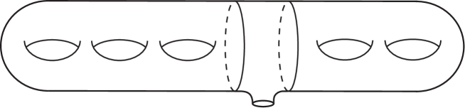
Figure 3: Gluing $S_{3,1}$ to $S_{2,1}$ to produce $S_{5,1}$.

This inclusion induces a map

$$\mathcal{I}_{g,1}\times\mathcal{I}_{h,1}\to\mathcal{I}_{g+h,1}$$ (11)

The pair-of-pants product

$$H_{i}(\mathcal{I}_{g,1})\times H_{j}(\mathcal{I}_{h,1})\to H_{i+j}(\mathcal{I}_{g+h,1})$$

is the map obtained by composing the Künneth map $H_{i}(\mathcal{I}_{g,1})\times H_{j}(\mathcal{I}_{h,1})\to H_{i+j}(\mathcal{I}_{g,1}\times\mathcal{I}_{h,1})$ with the map on homology induced by (11). Given $\sigma\in H_{i}(\mathcal{I}_{g,1})$ and $\eta\in H_{j}(\mathcal{I}_{h,1})$, we denote their pair-of-pants product by $\sigma\times\eta\in H_{i+j}(\mathcal{I}_{g+h,1})$.

Proposition 3.2.

Given $\sigma\in H_{i}(\mathcal{I}_{g,1})$ and $\eta\in H_{j}(\mathcal{I}_{h,1})$ with $i,j\geq 1$, we have$\tau_{i+j}(\sigma\times\eta)=0$.

Proof.

Let $S_{g,1}\to E^{\prime}_{\sigma}\to B_{\sigma}$ represent $[B_{\sigma}]\mapsto\sigma\in H_{i}(\mathcal{I}_{g,1})$, with $S_{g,*}\to E_{\sigma}\to B_{\sigma}$ representing $[B_{\sigma}]\mapsto\sigma\in H_{i}(\mathcal{I}_{g,*})$; similarly define $S_{g,1}\to E^{\prime}_{\eta}\to B_{\eta}$ and$S_{g,*}\to E_{\eta}\to B_{\eta}$. Let $[E_{\sigma}]\in H_{i+2}(E_{\sigma})$ be the preimage of $[B_{\sigma}]$ in $E_{\sigma}$, and similarly for $[E_{\eta}]\in H_{j+2}(E_{\eta})$. Let the bundle $S_{g+h,*}\to\overline{E}\to B_{\sigma}\times B_{\eta}$ represent $[B_{\sigma}]\times[B_{\eta}]\mapsto\sigma\times\eta\in H_{i+j}(\mathcal{I}_{g+h,*})$. The restriction of $\overline{E}$ to $B_{\sigma}$ is the bundle obtained by identifying $S_{g,1}\to E^{\prime}_{\sigma}\to B_{\sigma}$ with the trivial bundle $S_{h,1,*}\to S_{h,1,*}\times B_{\sigma}\to B_{\sigma}$ along their mutual boundary component $S^{1}\times B_{\sigma}$; a similar observation applies to the restriction to $B_{\eta}$.

The quotient $S_{g+h,*}\to S_{g}\vee S_{h}$ induces a quotient $\overline{E}\to Z$, where $Z$ is a bundle $S_{g}\vee S_{h}\to Z\to B_{\sigma}\times B_{\eta}$. The point where the two surfaces intersect gives a basepoint for $S_{g}\vee S_{h}$, and taking this point in each fiber yields a section of $Z$. Note that $Z$ is the union of two subspaces: the first a bundle $S_{g}\to Z_{1}\to B_{\sigma}\times B_{\eta}$, and the second a bundle $S_{h}\to Z_{2}\to B_{\sigma}\times B_{\eta}$. By inspection, we see that $Z_{1}$ is just $S_{g}\to E_{\sigma}\times B_{\eta}\to B_{\sigma}\times B_{\eta}$, and similarly $Z_{2}$ is $S_{h}\to B_{\sigma}\times E_{\eta}\to B_{\sigma}\times B_{\eta}$. The quotient $\overline{E}\to Z$ maps

$$[\overline{E}]\quad\mapsto\quad[E_{\sigma}]\times[B_{\eta}]\ +\ [B_{\sigma}]\times[E_{\eta}]\quad\in H_{i+j+2}(Z).$$

The parametrized Abel–Jacobi map $J_{\overline{E}}\colon Z\to T^{2g+2h}$ can be defined on $E_{\sigma}\times B_{\eta}$ by $J_{E_{\sigma}}\times 0$, and on $B_{\sigma}\times E_{\eta}$ by $0\times J_{E_{\eta}}$. It is easy to check that this is well-defined, and that it induces the appropriate map on fundamental group. From this formula, we see that the image under $J_{\overline{E}}$ of the first piece $E_{\sigma}\times B_{\eta}$ is contained in the image of $J_{E_{\sigma}}$, which has dimension at most $i+2$. Thus $[E_{\sigma}]\times[B_{\eta}]\in H_{i+j+2}(E_{\sigma}\times B_{\eta})$ is mapped to zero in $H_{i+j+2}(T^{2g+2h})$. The same applies to the second piece $B_{\sigma}\times E_{\eta}$, and so we have

$$\tau_{i+j}(\sigma\times\eta)=(J_{\overline{E}})_{*}[\overline{E}]=(J_{\overline{E}})_{*}([E_{\sigma}]\times[B_{\eta}])+(J_{\overline{E}})_{*}([B_{\sigma}]\times[E_{\eta}])=0+0=0$$

as desired. ∎

Abelian cycles. A collection of commuting elements $f_{1},\ldots,f_{d}$ of a group $G$ induces a map $\mathbb{Z}^{d}\to G$; we denote the image of the fundamental class $[\mathbb{Z}^{d}]\in H_{d}(\mathbb{Z}^{d},\mathbb{Q})$ in $H_{d}(G,\mathbb{Q})$ by $\{f_{1},\ldots,f_{d}\}$. This is called an abelian cycle in $H_{d}(G,\mathbb{Q})$. Proposition 3.1 and Proposition 3.2 can be used to compute $\tau_{i}$ on certain abelian cycles.

Definition 3.3.

Let $f_{1},\ldots,f_{k}$ be a collection of bounding pair maps on $S_{g,*}$, with $f_{i}$ being the twist about $\alpha_{i}$ composed with the inverse twist about $\beta_{i}$. Recall that the curves $\alpha_{i},\beta_{i}$ are assumed to be nonseparating. We say that this collection is truly nested if

1. the curves $\alpha_{i}$ are pairwise non-homologous, and

2. after possibly re-ordering $\{f_{i}\}$, the union $\alpha_{j}\cup\beta_{j}$ separates the basepoint from $\alpha_{i}\cup\beta_{i}$ whenever $i<j$.

An easy induction shows that these conditions force the curves $\alpha_{i}$ and $\beta_{i}$ to be in one of the “standard configurations”, a representative example of which is given in Figure 4a. Note that, by this definition, a single bounding pair map is truly nested. For further examples, the collections depicted in Figures 5a, 6, 7, and 9 are truly nested, while the collection depicted in Figure 8 is not. We assume that any truly nested collection has been reordered so that the second condition above holds.

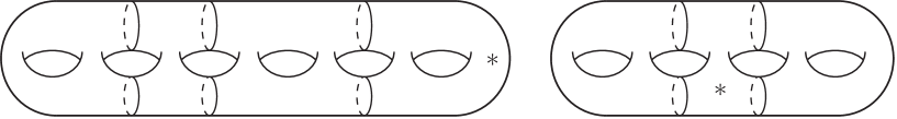
Figure 4: The first collection is truly nested; the second collection is not.

For any bounding pair $f_{i}$, let $c_{i}$ be the common homology class of $\alpha_{i}$ and $\beta_{i}$. If a collection is truly nested (and ordered as above), then consider the “farthest” subsurface cut off, namely the component of $S_{g,*}\setminus(\alpha_{1}\cup\beta_{1})$ not containing the basepoint. Choose $S_{0}$ to be a surface with one boundary component, contained in the “farthest” subsurface, of maximal genus. Let $\omega_{0}\in\textstyle{\bigwedge}^{2}H_{1}(S_{0})\subset\textstyle{\bigwedge}^{2}H_{1}(S_{g,*})$ be a symplectic form for $H_{1}(S_{0})$. Note that the subspace $H_{1}(S_{0})$ is not uniquely determined. However, the following theorem holds regardless of the choice of $S_{0}$.

Theorem 3.4.

Any truly nested collection of bounding pair maps determines a nonzero abelian cycle. More precisely, with notation as above, the image under $\tau_{k}$ of the abelian cycle $\{f_{1},\ldots,f_{k}\}$ is

$$\tau_{k}(\{f_{1},\ldots,f_{k}\})=\omega_{0}\wedge c_{1}\wedge\cdots\wedge c_{k}.$$

Proof.

Let $S_{0}$ be as above. For $1\leq i\leq k$, sequentially choose $S_{i}$ to be a subsurface of $S_{g,1}$ with one boundary component and maximal genus subject to the condition that $S_{i}$ contains $\alpha_{j}\cup\beta_{j}$ for all $j\leq i$, $S_{i}$ contains $S_{i-1}$, and $S_{i}$ is disjoint from $\alpha_{j}\cup\beta_{j}$ for all $j>i$. The existence of such subsurfaces $S_{i}$ follows from the assumption that the collection is truly nested. Note that $S_{k}$ is the whole surface $S_{g,1}$.

Let $1\in H_{0}(\mathcal{I}(S_{0}))$ be a generator. By Proposition 2.1, $\tau_{0}(1)=\omega_{0}$. For each $0\leq i\leq k$, the abelian cycle $\{f_{1},\ldots,f_{i}\}$ may be considered as an element of $H_{i}(\mathcal{I}(S_{i}))$. We show by induction that $\tau_{i}(\{f_{1},\ldots,f_{i}\})=\omega\wedge c_{1}\wedge\cdots\wedge c_{i}$. The abelian cycle $\{f_{1},\ldots,f_{i+1}\}$ can be written as the cross product $\{f_{1},\ldots,f_{i}\}\times f_{i+1}$ in the sense of Proposition 3.1, followed by the map to $H_{i+1}(S_{i+1})$ induced by the inclusion of the subsurface. The inductive step follows by applying Proposition 3.1. ∎

Conversely, we have the following.

Theorem 3.5.

If $f_{1},\ldots,f_{k}$ is a collection of commuting bounding pair maps that is not truly nested, then

$$\tau_{k}(\{f_{1},\ldots,f_{k}\})=0.$$

Proof.

A collection which is not truly nested must fail either the first or second condition in Definition 3.3.

Case I. We prove the following (a priori stronger) claim: if the homology classes of the curves $\alpha_{1},\ldots,\alpha_{k}$ are not linearly independent, then $\tau_{i}(\{f_{1},\ldots,f_{k}\})=0$. Let $m$ be the rank of the span of the homology classes $c_{1},\ldots,c_{k}$, and let $\gamma_{1},\ldots,\gamma_{2k}$ be the $\alpha_{i}$ and $\beta_{i}$, ordered arbitrarily. We will prove below that it is possible to choose curves $\delta_{1},\ldots,\delta_{2g}$ with the following properties:

1. their homology classes $d_{1},\ldots,d_{2g}$ are a symplectic basis for $H_{1}(S_{g})$, so that $(d_{i},d_{g+i})=1$ for $1\leq i\leq g$;

2. for $i\leq m$ each curve $\delta_{i}$ is one of the $\gamma_{j}$;

3. the span of $\langle d_{1},\ldots,d_{m}\rangle$ is the span of $\langle c_{1},\ldots,c_{k}\rangle$;

4. the curve $\delta_{i}$ is disjoint from all the curves $\gamma_{j}$ for all $i$ except $g+1\leq i\leq g+m$.

Given such a collection $\delta_{1},\ldots,\delta_{2g}$, we construct an Abel–Jacobi map $j\colon(S_{g},\ast)\to(T^{2g},0)$ supported on a neighborhood of the union $\delta_{1}\cup\cdots\cup\delta_{2g}$. One way to do this is to choose $1$–forms $\theta_{i}$ dual to $\delta_{i}$ and supported in a small neighborhood. Then $j$ is defined by:

$$j(p)=\left(\int_{\ast}^{p}\theta_{g+1}\,,\ \ldots\,,\ \int_{\ast}^{p}\theta_{2g}\,,\,\int_{\ast}^{p}-\theta_{1}\,,\ \ldots\,,\ \int_{\ast}^{p}-\theta_{g}\right)$$

By transversality, we may assume that the curves $\delta_{i}$ intersect at most pairwise; it follows that the image $j(S_{g})$ is contained in the $2$–skeleton of $T^{2g}$.

Consider the bundle $S_{g,*}\to E\to T^{k}$ representing $\{f_{1},\ldots,f_{k}\}\in H_{k}(\mathcal{I}_{g,*})$. As in the proof of Proposition 2.2, we may use the map $j$ to construct a parametrized Abel–Jacobi map $J_{E}\colon E\to T^{2g}$. The disjointness properties of $\delta_{i}$ imply that for each $\ell$, $j\circ f_{\ell}-j$ is nonzero only in the components determined by $d_{1},\ldots,d_{m}$. It follows from the construction of $J$ that the image $J_{E}(E)$ is contained in the finite union of the tori (of dimension at most $m+2$) determined by the components $d_{1},\ldots,d_{m}$ together with at most two other basis elements $d_{i}$ and $d_{j}$. This subcomplex of $T^{2g}$ has dimension $m+2$; since $m<k$, it follows that $(J_{E})_{*}[E]=0$ in $H_{k+2}(T^{2g})$.

We now show how to find such a collection $\delta_{i}$. We first find $\delta_{m+1},\ldots,\delta_{g}$ and $\delta_{g+m+1},\ldots,\delta_{2g}$ as follows. Consider again the complement $S_{g,1}\setminus\bigcup\gamma_{i}$. Each component of the complement is a surface of some genus $g_{j}\geq 0$; we may easily find $g_{j}$ pairs of curves on this subsurface, each pair intersecting in one point, and whose homology classes are a symplectic basis for the subspace they span. The claim is that doing so on each complementary subsurface yields $g-m$ such pairs. By collapsing to a point the genus 1 subsurface which is a regular neighborhood of such a pair, we may assume that each complementary subsurface has genus 0; to prove the claim, we need to prove that $m=g$ under this assumption. Consider the functionals $H_{1}(S_{g,1})\to\mathbb{Q}$ given by intersection with each of the $\gamma_{i}$. The space of functionals spanned by this collection has rank $m$. But if the complementary components have genus 0, their homology is spanned by the homology of their boundary components. Then Mayer–Vietoris implies that the mutual kernel of all these functionals is generated by the boundary components $\gamma_{i}$, and thus has rank $m$. We conclude that $H_{1}(S_{g,1})$ has rank $2m$; this verifies the claim, and so we have $g-m$ pairs of curves, which we take as $\delta_{m+1},\ldots,\delta_{g}$ and $\delta_{g+m+1},\ldots,\delta_{2g}$. At this point it is easy to choose $\delta_{1},\ldots,\delta_{m}$ and $\delta_{g},\ldots,\delta_{g+m}$. For the former, we choose any $m$ curves from the $\gamma_{j}$ whose homology classes are linearly independent to be $\delta_{1},\ldots,\delta_{m}$. Now the only condition on the remaining curves is that their homology classes should make $d_{1},\ldots,d_{2g}$ a symplectic basis, so we may choose $\delta_{g+m+1},\ldots,\delta_{2g}$ arbitrarily subject to this condition. This completes the proof in the first case.

Case II. Now consider the case when the second condition is violated. We explain first the case when no bounding pair separates the basepoint from the others. Consider the component $C$ of $S_{g,1}\setminus\bigcup\gamma_{i}$ which is adjacent to the boundary component. The boundary of $C$ consists of curves $\alpha_{i}$ or $\beta_{j}$ (plus $\partial S_{g,1})$, and under our assumptions it contains curves from at least two bounding pairs. There must be some bounding pair $f_{i}$ so that $C$ contains both $\alpha_{i}$ and $\beta_{i}$; otherwise, without loss of generality the boundary of $C$ would consist of $\alpha_{1},\ldots,\alpha_{j}$ for some $j$, plus $\partial S_{g,1}$. But then the homology classes of these curves would be linearly dependent, and this case has already been dealt with. Thus $C$ contains both $\alpha_{i}$ and $\beta_{i}$ for some $i$, and so there is a separating curve $\gamma$ in $C$ cutting off exactly $\alpha_{i}$ and $\beta_{i}$. Extend this arbitrarily to a pair-of-pants $S_{0,3}$ contained in $C$ having both $\gamma$ and $\partial S_{g,1}$ as boundary components.

Note that $S_{g,1}\setminus S_{0,3}$ has two components $S_{h,1}$ and $S_{g-h,1}$, each of which contains at least one bounding pair. Relabeling, we may assume that $f_{1},\ldots,f_{j}$ are contained in $S_{h,1}$ and $f_{j+1},\ldots,f_{k}$ are contained in $S_{g-h,1}$ for $0<j<k$. Then the abelian cycle $\{f_{1},\ldots,f_{k}\}\in H_{k}(\mathcal{I}_{g,1})$ is obtained as the pair-of-pants product of $\{f_{1},\ldots,f_{j}\}\in H_{j}(\mathcal{I}_{h,1})$ and $\{f_{j+1},\ldots,f_{k}\}\in H_{k-j}(\mathcal{I}_{g-h,1})$. Applying Proposition 3.1, we conclude that $\tau_{k}(\{f_{1},\ldots,f_{k}\})=0$.

In general such a configuration will be present, but not necessarily adjacent to the basepoint. We attempt to order the bounding pairs inductively as $f_{k}$, $f_{k-1}$, etc., so that for each $i$ the union $\alpha_{i}\cup\beta_{i}$ separates the basepoint from all bounding pairs not yet labeled. Since the collection is not truly nested, at some point we cannot continue this process; we are left with some subset $\{f_{1},\ldots,f_{\ell}\}$ which cannot be so ordered. Let $S_{\ell}$ be a subsurface with one boundary component and maximal genus subject to the condition that $S_{\ell}$ contains $\alpha_{i}\cup\beta_{i}$ if $i\leq\ell$ and is disjoint from $\alpha_{i}\cup\beta_{i}$ for $i>\ell$. Then $\{f_{1},\ldots,f_{\ell}\}\in H_{\ell}(\mathcal{I}(S_{\ell}))$ is as discussed in the previous two paragraphs, and so $\tau_{\ell}(\{f_{1},\ldots,f_{\ell}\})=0$. Now just as in the proof of Theorem 3.4, we may filter $S_{g,1}$ by nested subsurfaces $S_{i}$ for $\ell\leq i\leq k$ with $S_{i}$ containing $\alpha_{j}\cup\beta_{j}$ iff $j\leq i$. As before, $\{f_{1},\ldots,f_{i+1}\}$ is the cross product $\{f_{1},\ldots,f_{i}\}\times f_{i+1}$, so applying Proposition 3.1, we have by induction

$$\tau_{i+1}(\{f_{1},\ldots,f_{i+1}\})=\tau_{i}(\{f_{1},\ldots,f_{i}\})\wedge c_{i}=0\wedge c_{i}=0.\qed$$

Separating twists. We can try to generalize these techniques beyond bounding pair maps. In general, given $f\in\mathcal{I}_{g,\ast}$ and $\sigma\in H_{i}(\mathcal{I}_{g,\ast})$, we cannot form $\sigma\times f\in H_{i+1}(\mathcal{I}_{g,\ast})$. However, consider the inclusion of the centralizer $C_{\mathcal{I}}(f)$ into $\mathcal{I}_{g,\ast}$; if $\sigma$ is represented by some $\widetilde{\sigma}\in H_{i}(C_{\mathcal{I}}(f))$, we can consider $\widetilde{\sigma}\times f\in H_{i+1}(C_{\mathcal{I}}(f)\times\langle f\rangle)$ and define its image to be $\sigma\times f\in H_{i+1}(\mathcal{I}_{g,\ast})$. Of particular importance is the case when $f$ is a twist $T_{\gamma}$ about a separating curve. However, unlike bounding pair maps, separating twists do not produce nontrivial abelian cycles with respect to $\tau_{i}$.

Proposition 3.6.

Let $T_{\gamma}$ be the Dehn twist about a separating curve $\gamma$, and let$\sigma\in H_{i}(\mathcal{I}_{g,*})$ be such that $\sigma\times T_{\gamma}$ is well-defined. Then $\tau_{i+1}(\sigma\times T_{\gamma})=0$.

Proof.

Let $S_{g,*}\to E\to B$ represent $[B]\mapsto\sigma$. By assumption we may assume that the classifying map factors through $C_{\mathcal{I}}(f)$, so the entire image of $\pi_{1}(B)\to\mathcal{I}_{g,*}$ fixes the curve $\gamma$. Thus by fiberwise collapsing $\gamma$ to a point, we have the quotient $E\to Y$, where $Y$ fibers as

$$S_{h}\vee S_{g-h}\to Y\to B$$

for some $1\leq h<g$. This is the union of two subspaces, $S_{h}\to Y_{1}\to B$ and $S_{g-h}\to Y_{2}\to B$. Since $\gamma$ is separating, we may start with an Abel–Jacobi map $j\colon S_{g,*}\to T^{2g}$ so that $\gamma$ is mapped to 0, so we can find a parametrized Abel–Jacobi map $J_{E}\colon E\to T^{2g}$ which factors through $Y$.

The class $\sigma\times T_{\gamma}$ is represented by $S_{g,*}\to\overline{E}\to B\times S^{1}$, where as above $\overline{E}=E\times[0,1]/(T_{\gamma}(p),0)\sim(p,1)$. As above, $\overline{E}$ descends to a quotient $S_{h}\vee S_{g-h}\to Z\to B\times S^{1}$. This is the union of two subspaces, which are easily seen to be products $Y_{1}\times S^{1}$ and $Y_{2}\times S^{1}$. We may define $J_{\overline{E}}\colon Z\to T^{2g}$ on both $Y_{1}\times S^{1}$ and $Y_{2}\times S^{1}$ by $J_{E}\times 0$. Thus $J_{\overline{E}}$ factors through the $(i+2)$–dimensional complex $Y$, and so

$$\tau_{i+1}(\sigma\times T_{\gamma})=(J_{\overline{E}})_{*}[\overline{E}]=0.\qed$$

4 The Gysin homomorphism and $\tau_{i}$

In this section we show how the Gysin homomorphism can be used to construct nonzero cycles detectable by $\tau_{i}$. To this end, consider the universal surface bundle

$$1\to S_{g}\to\operatorname{{\cal T}}_{g,*}\overset{\pi}{\to}\operatorname{{\cal T}}_{g}\to 1.$$

We then have the Gysin homomorphism $\pi^{!}\colon H_{i}(\mathcal{I}_{g})\to H_{i+2}(\mathcal{I}_{g,*})$; by precomposing with the map $H_{i}(\mathcal{I}_{g,*})\to H_{i}(\mathcal{I}_{g})$ induced by $\pi$, we can also consider $\pi^{!}$ as a map $H_{i}(\mathcal{I}_{g,*})\to H_{i+2}(\mathcal{I}_{g,*})$. Composing with $\tau_{i+2}$ we obtain

$$\tau_{i+2}\circ\pi^{!}\colon H_{i}(\mathcal{I}_{g,\ast})\to\textstyle{\bigwedge}^{i+4}H.$$

We can use this map to detect new nontrivial cycles in $H_{i+2}(\mathcal{I}_{g,\ast})$. Let $\{f_{1},\ldots,f_{k}\}$ be a truly nested collection of bounding pair maps with homology classes $c_{1},\ldots,c_{k}$. As before, consider the component of $S_{g}\setminus(\alpha_{1}\cup\beta_{1})$ not containing the basepoint (the “farthest” subsurface), let $S_{0}$ be a maximal subsurface with one boundary component, and let $\omega_{0}$ represent the symplectic form on $H_{1}(S_{0})$. Similarly, consider the component of $S_{g}\setminus(\alpha_{k}\cup\beta_{k})$ containing the basepoint (the “closest” subsurface), let $S^{0}$ be a maximal subsurface with one boundary component, and let $\omega^{0}$ represent the symplectic form on $H_{1}(S^{0})$. The following theorem holds regardless of the choice of $S_{0}$ and $S^{0}$.

Theorem 4.1.

Let $k\geq 2$ be even, and let $\{f_{1},\ldots,f_{k}\}$ be a truly nested collection of bounding pair maps with homology classes $c_{1},\ldots,c_{k}$. Then with $\omega_{0}$ and $\omega^{0}$ as above,

$$\tau_{k+2}\big{(}\pi^{!}\{f_{1},\ldots,f_{k}\}\big{)}=2\cdot\omega_{0}\wedge\omega^{0}\wedge c_{1}\wedge\cdots\wedge c_{k}.$$

In contrast, when $k$ is odd, we have the following theorem.

Theorem 4.2.

If $k$ is odd, then $\tau_{k+2}\circ\pi^{!}$ is the zero map.

Before proving these theorems, we interpret $\pi^{!}$ in terms of bundles as above. The composition $\operatorname{{\cal T}}_{g,*}^{*}\to\operatorname{{\cal T}}_{g,*}\to\operatorname{{\cal T}}_{g}$ yields (as we will show in the following two paragraphs) a fiber bundle $S_{g}\times S_{g}\to\operatorname{{\cal T}}_{g,*}^{*}\overset{\Pi}{\to}\operatorname{{\cal T}}_{g}$ with associated Gysin homomorphism $\Pi^{!}\colon H_{i}(\mathcal{I}_{g})\to H_{i+4}(\mathcal{I}_{g,*}^{*})$. Recall that $J\colon\mathcal{I}_{g,*}^{*}\to H_{\mathbb{Z}}$ is the homomorphism which is the abelianization on the fiber and trivial on the subgroup $\mathcal{I}_{g,*}$. By definition, we have

$$\tau_{k+2}\circ\pi^{!}=J_{*}\circ\Pi^{!}\colon H_{k}(\mathcal{I}_{g})\to H_{k+4}(\mathcal{I}_{g,*}^{*})\to H_{k+4}(H_{\mathbb{Z}})\approx\textstyle{\bigwedge}^{k+4}H.$$

This can be described explicitly in terms of bundles, as follows.

Let $S_{g}\to E\to B$ represent $[B]\mapsto\sigma\in H_{k}(\mathcal{I}_{g})$, with $[E]\in H_{k+2}(E)$ denoting the preimage of $[B]$. Let $S_{g}\to\overline{E}\to E$ be the pullback of $S_{g}\to E\to B$ to $E$ by the map $p\colon E\to B$, and let $[\overline{E}]\in H_{k+4}(\overline{E})$ be the preimage of $[E]$. This pullback consists of pairs of points $(e_{1},e_{2})\in E\times E$ such that $p(e_{1})=p(e_{2})$. Thus the “diagonal” consisting of pairs $(e,e)$ gives a section $s\colon E\to\overline{E}$ of the bundle $S_{g}\to\overline{E}\to E$. In summary, we have the following diagram:

By composing with the map $E\to B$, we can consider $\overline{E}$ as a bundle over $B$. The fiber $F$ is a bundle-with-section of the form $S_{g,*}\to F\to S_{g}$. It can be verified that the monodromy $\pi_{1}(S_{g},\ast)\to\operatorname{Mod}_{g,*}$ is contained in the kernel of the natural map $\operatorname{Mod}_{g,*}\to\operatorname{Mod}_{g}$ (it is easy to check that this kernel is contained in $\mathcal{I}_{g,*}$). Indeed Birman proved (see, e.g. [FM, Theorem 4.6]) that this map gives an isomorphism

$$\pi_{1}(S_{g},\ast)\approx\ker(\operatorname{Mod}_{g,*}\to\operatorname{Mod}_{g})$$ (12)

It thus follows that as a surface bundle, $F\approx S_{g}\times S_{g}$. The section $s$ intersects each fiber $F$ in the diagonal $\Delta\subset S_{g}\times S_{g}$.

Since $[\overline{E}]=\Pi^{!}([B])$, we have that $\tau_{k+2}(\pi^{!}(\sigma))$ is the image of $[\overline{E}]$ under the parametrized Abel–Jacobi map $J_{\overline{E}}\colon\overline{E}\to T^{2g}$, which can be constructed as follows. Let $J_{E}\colon E\to T^{2g}$ be a parametrized Abel–Jacobi map, and define $J_{\overline{E}}\colon\overline{E}\to T^{2g}$ to be

$$J_{\overline{E}}\big{(}(e_{1},e_{2})\big{)}=J_{E}(e_{1})-J_{E}(e_{2}).$$

As above, to verify that $J_{\overline{E}}$ is the parametrized Abel–Jacobi map for $\overline{E}$, we need to check that the induced map on fundamental group is trivial when restricted to the section $s$, and is the abelianization when restricted to a fiber $S_{g}$. The former is immediate, since $s$ consists of pairs $(e,e)$. The fiber $S_{g}$ is the set of pairs $\{(e,e_{0})\}$ in $\overline{E}$, for some fixed $e_{0}\in E$. The map $e\mapsto(e,e_{0})$ identifies this with the fiber of $E$ containing $e_{0}$. Note that since $J_{E}$ is a parametrized Abel–Jacobi map for $E$, its restriction to a fiber induces the abelianization. Since $J_{\overline{E}}\big{(}(e,e_{0})\big{)}=J_{E}(e)-J_{E}(e_{0})$, the restriction of $J_{\overline{E}}$ to this fiber $S_{g}$ is the translate of $J_{E}$ by the constant $-J_{E}(e_{0})$. Thus when restricted to this fiber, $J_{\overline{E}}$ is homotopic to $J_{E}$ and thus induces the same map on the fundamental group.

With this description in terms of bundles in hand, we can now prove the theorems stated above.

Proof of Theorem 4.2.

The bundle $S_{g}\times S_{g}\to\overline{E}\to B$ admits a natural involution $\rho\colon\overline{E}\to\overline{E}$ defined by $\rho\big{(}(e_{1},e_{2})\big{)}=(e_{2},e_{1})$. Note that $\rho$ covers the identity $B\to B$. Restricted to a fiber, this is just the transposition of coordinates $S_{g}\times S_{g}\to S_{g}\times S_{g}$. Since $S_{g}$ is even-dimensional, this homeomorphism is orientation-preserving, and so it fixes the fundamental class $[S_{g}\times S_{g}]\in H_{4}(S_{g}\times S_{g})$. Thus by the naturality of the Gysin homomorphism (see e.g. [Mo01, Proposition 4.8(iii)]) we have $\rho_{*}\circ\Pi^{!}=\Pi^{!}$. Define $\nu\colon T^{2g}\to T^{2g}$ to be the map induced by the map $\mathbb{R}^{2g}\to\mathbb{R}^{2g}$ given by $v\mapsto-v$. Note that $\nu_{*}\colon H_{k}(T^{2g})\to H_{k}(T^{2g})$ is the identity when $k$ is even, and is minus the identity when $k$ is odd. From the way we constructed $J_{\overline{E}}$, we see that

$$J_{\overline{E}}\circ\rho=\nu\circ J_{\overline{E}}.$$

But now we have

$$(J_{\overline{E}})_{*}\circ\Pi^{!}=(J_{\overline{E}})_{*}\circ\rho_{*}\circ\Pi^{!}=\nu_{*}\circ(J_{\overline{E}})_{*}\circ\Pi^{!}$$

Thus when $k$ is odd, we have $(J_{\overline{E}})_{*}\circ\Pi^{!}=-(J_{\overline{E}})_{*}\circ\Pi^{!}$, which implies

$$\tau_{k+2}\circ\pi^{!}=(J_{\overline{E}})_{*}\circ\Pi^{!}=0$$

as desired. ∎

Proof of Theorem 4.1.

Let $S_{g}\to E\to T^{k}$ be the bundle classifying the abelian cycle $\sigma=\{f_{1},\ldots,f_{k}\}\in H_{k}(\mathcal{I}_{g})$. Form as above the fiber product bundle $S_{g}\to\overline{E}\to E$ representing $\pi^{!}(\sigma)$, and view it as a bundle $S_{g}\times S_{g}\to\overline{E}\to T^{k}$. The parametrized Abel–Jacobi map $J_{\overline{E}}\colon\overline{E}\to T^{2g}$ can be defined as in the proof of Proposition 2.2. We construct $\overline{E}$ as

$$S_{g}\times S_{g}\times[0,1]^{k}/\sim$$

where

$$(p,q,t_{1},\ldots,t_{i-1},0,t_{i+1},\ldots,t_{k})\sim(f_{i}(p),f_{i}(q),t_{1},\ldots,t_{i-1},1,t_{i+1},\ldots,t_{k}).$$

Let $j\colon S_{g}\to T^{2g}$ be the Abel–Jacobi map, and let $\delta_{i}\colon S_{g}\to\mathbb{R}^{2g}$ be the unique map satisfying $j\circ f_{i}=j+\delta_{i}\bmod{\mathbb{Z}^{2g}}$ and $\delta_{i}(\ast)=0$. Then $J_{\overline{E}}$ can now be defined by

$$J_{\overline{E}}\big{(}(p,q,t_{1},\ldots,t_{k})\big{)}=j(p)-j(q)+\sum_{i}t_{i}\big{(}\delta_{i}(p)-\delta_{i}(q)\big{)}.$$

The definition of $\delta_{i}$ was chosen exactly so that this descends to a map $J_{\overline{E}}\colon\overline{E}\to T^{2g}$.

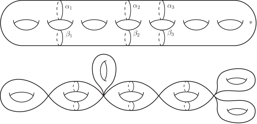
Figure 5: a. The bounding pair maps $f_{i}$. b. The quotient $Y=\bigcup T_{\ell}$.

Any truly nested collection of bounding pairs is, up to homeomorphism, of the form depicted in Figure 5a. The maps $f_{i}$ factors through a union of 2–dimensional tori $Y=\bigcup T_{\ell}$, any two of which meet in at most one point, as depicted in Figure 5b. We have a basis $\{a_{1},b_{1},\ldots,a_{g},b_{g}\}$ for $H$ so that $a_{\ell}$ and $b_{\ell}$ span the homology of the torus $T_{\ell}$. For each bounding pair map $f_{i}$, the homology class $c_{i}$ of its defining pair of curves is equal to $a_{\ell_{i}}$ for some $\ell_{i}$. As in the definition of a truly nested collection, we assume that $\ell_{i}<\ell_{i^{\prime}}$ if $i<i^{\prime}$; for simplicity, we order the $T_{\ell}$ so that $T_{\ell}$ is separated from the basepoint by $T_{\ell_{i}}$ iff $\ell<\ell_{i}$.

We can choose $j$ so that $j$, and thus also the $\delta_{i}$, factors through $Y$, and furthermore so that as in Proposition 2.2, $j$ and $j\circ f_{i}$ differ only in the component corresponding to $a_{\ell_{i}}$. The restriction of $j$ to the torus $T_{\ell}$ gives an identification with the linear subspace of $T^{2g}$ consisting of the $\langle a_{\ell},b_{\ell}\rangle$ plane; parametrizing $T_{\ell}$ by this identification, we have that the restriction of $j$ to $T_{\ell}$ is just the inclusion of this subspace.

It follows that $J_{\overline{E}}$ factors through a space $Z$ which fibers as a bundle$Y\times Y\to Z\to T^{k}$; call the resulting map $J_{Z}\colon Z\to T^{2g}$. This bundle is the union of subspaces of the form $T_{\ell}\times T_{\ell^{\prime}}\to Z_{\ell,\ell^{\prime}}\to T^{k}$; the intersection of two such subspaces has codimension at least 2, corresponding to $T_{\ell_{1}}\times T_{\ell^{\prime}}\cap T_{\ell_{2}}\times T_{\ell^{\prime}}=\ast\times T_{\ell^{\prime}}$ or to $T_{\ell_{1}}\times T_{\ell_{1}^{\prime}}\cap T_{\ell_{2}}\times T_{\ell_{2}^{\prime}}=\ast\times\ast$. It follows that the fundamental class $[\overline{E}]\in H_{k+4}(\overline{E})$ projects to the sum of the fundamental classes $\sum[Z_{\ell,\ell^{\prime}}]\in H_{k+4}(Z)$. Thus to compute $\tau_{k+2}(\pi^{!}\{f_{1},\ldots,f_{k}\})=(J_{\overline{E}})_{*}[\overline{E}]$, it remains to understand $(J_{Z})_{*}[Z_{\ell,\ell^{\prime}}]$.

Call the subspace $Z_{\ell,\ell^{\prime}}$ bad if either $\ell$ or $\ell^{\prime}$ is equal to $\ell_{i}$ for some $i$; otherwise call $Z_{\ell,\ell^{\prime}}$ good. First, let us check that for bad $Z_{\ell,\ell^{\prime}}$, we have $(J_{Z})_{*}[Z_{\ell,\ell^{\prime}}]=0$. For $(p,q,t_{1},\ldots,t_{k})\in Z_{\ell,\ell^{\prime}}$ we have $p\in T_{\ell}$ and $q\in T_{\ell^{\prime}}$; thus $j(p)$ and $j(q)$ are contained in the subspace determined by $\langle a_{\ell},b_{\ell}\rangle$ and $\langle a_{\ell^{\prime}},b_{\ell^{\prime}}\rangle$ respectively. Recall that each $\delta_{i}$ is nonzero only in the coordinate corresponding to $c_{i}$. Our formula for $J_{\overline{E}}((p,q,t_{1},\ldots,t_{k}))$ thus implies that $J_{Z}(Z_{\ell,\ell^{\prime}})$ is contained in the subspace determined by the collection $\langle a_{\ell},b_{\ell},a_{\ell^{\prime}},b_{\ell^{\prime}},c_{1},\ldots,c_{k}\rangle$. However, the assumption that $Z_{\ell,\ell^{\prime}}$ is bad implies that $a_{\ell}$ or $a_{\ell^{\prime}}$ coincides with some $c_{i}$. Thus this subspace has dimension at most $k+3$, and so $(J_{Z})_{*}[Z_{\ell,\ell^{\prime}}]\in H_{k+4}(T^{2g})$ must be zero.

Now we consider the good pieces $Z_{\ell,\ell^{\prime}}$. Since neither $\ell$ nor $\ell^{\prime}$ is of the form $\ell_{i}$ for any $i$, we have that each map $f_{i}$ is the identity on $T_{\ell}$ and $T_{\ell^{\prime}}$. It follows that the bundle $T_{\ell}\times T_{\ell^{\prime}}\to Z_{\ell,\ell^{\prime}}\to T^{k}$ is actually a product $Z_{\ell,\ell^{\prime}}\approx T_{\ell}\times T_{\ell^{\prime}}\times T^{k}$. Note that since $j\circ f_{i}=j$ on $T_{\ell}$, we have that each $\delta_{i}$ is constant on $T_{\ell}$ and is nonzero only in the component corresponding to $c_{i}$. In that component, we have as before that $\delta_{i}$ is either $1$ or $0$ on $T_{\ell}$, depending on whether the torus $T_{\ell}$ is cut off from the basepoint by $\alpha_{i}\cup\beta_{i}$ or not. Denoting this number by $n^{i}_{\ell}\in\{0,1\}$, we see that $n^{i}_{\ell}$ is $1$ if $\ell<\ell_{i}$ and is $0$ if $\ell_{i}<\ell$.

The restriction of $J_{Z}$ to $Z_{\ell,\ell^{\prime}}\approx T_{\ell}\times T_{\ell^{\prime}}\times T^{k}$ may now be read off from the formula for $J_{\overline{E}}$ above. The restriction is a linear map, which can be described on each factor. On the first and second factors, it is the inclusion of $T_{\ell}$ as the torus determined by $\langle a_{\ell},b_{\ell}\rangle$ and the inclusion of $T_{\ell^{\prime}}$ as the torus determined by $\langle a_{\ell^{\prime}},b_{\ell^{\prime}}\rangle$ respectively. Let $\varepsilon_{i}\in\{-1,0,1\}$ be the number $n^{i}_{\ell}-n^{i}_{\ell^{\prime}}$. On the third factor $T^{k}$, $J_{Z}$ is the composition of the map $T^{k}\to T^{k}$ given by

$$(t_{1},\ldots,t_{k})\mapsto(\varepsilon_{1}t_{1},\ldots,\varepsilon_{k}t_{k})$$ (13)

with the inclusion of $T^{k}$ as the torus determined by $\langle c_{1},c_{2},\ldots,c_{k}\rangle$. Note that the map $H_{k}(T^{k})\to H_{k}(T^{k})$ induced by (13) is multiplication by $\varepsilon_{\ell,\ell^{\prime}}=\varepsilon_{1}\cdots\varepsilon_{k}$. From this description we see that the image of the fundamental class $[Z_{\ell,\ell^{\prime}}]$ under $J_{Z}$ is

$$(J_{Z})_{*}[Z_{\ell,\ell^{\prime}}]=\varepsilon_{\ell,\ell^{\prime}}\cdot a_{\ell}\wedge b_{\ell}\wedge a_{\ell^{\prime}}\wedge b_{\ell^{\prime}}\wedge c_{1}\wedge\cdots\wedge c_{k}.$$

It thus remains only to understand $\varepsilon_{\ell,\ell^{\prime}}$. Since $n^{i}_{\ell}$ is $1$ if $\ell<\ell_{i}$ and $0$ otherwise, we have that $\varepsilon_{i}$ is 1 if $\ell<\ell_{i}<\ell^{\prime}$, $-1$ if $\ell^{\prime}<\ell_{i}<\ell$, and 0 otherwise. Thus $\varepsilon_{\ell,\ell^{\prime}}$ is nonzero only if we have $\ell<\ell_{1}<\cdots<\ell_{k}<\ell^{\prime}$ or $\ell^{\prime}<\ell_{1}<\cdots<\ell_{k}<\ell$. In the former case, each $\varepsilon_{i}=1$, so $\varepsilon_{\ell,\ell^{\prime}}=1$; in the latter, each $\varepsilon_{i}=-1$, but since $k$ is even we have $\varepsilon_{\ell,\ell^{\prime}}=\varepsilon_{1}\cdots\varepsilon_{k}=1$ again. Note that if $k$ were odd, these terms would instead cancel, yielding another proof of Theorem 4.2 (for the case of abelian cycles of bounding pairs). Combining these cases, we conclude that

$$J_{\overline{E}}\colon[\overline{E}] \mapsto\sum_{\ell,\ell^{\prime}}[Z_{\ell,\ell^{\prime}}]$$

$$\mapsto\sum_{\ell<\ell_{1}<\cdots<\ell_{k}<\ell^{\prime}}2\cdot a_{\ell}\wedge b_{\ell}\wedge a_{\ell^{\prime}}\wedge b_{\ell^{\prime}}\wedge c_{1}\wedge\cdots\wedge c_{k}$$

$$=2\cdot\omega_{0}\wedge\omega^{0}\wedge c_{1}\wedge\cdots\wedge c_{k}$$

and thus, as desired,

$$\tau_{k+2}\big{(}\pi^{!}\{f_{1},\ldots,f_{k}\}\big{)}=2\cdot\omega_{0}\wedge\omega^{0}\wedge c_{1}\wedge\cdots\wedge c_{k}.\qed$$

This proof is valid for $k=0$ as well, except for the last equality above; in this case we instead have just

$$\sum_{\ell<\ell^{\prime}}2\cdot a_{\ell}\wedge b_{\ell}\wedge a_{\ell^{\prime}}\wedge b_{\ell^{\prime}}=\omega\wedge\omega.$$

Thus if $[S_{g}]\in H_{2}(\mathcal{I}_{g,*})$ represents the point-pushing subgroup as in (12), we deduce the following, which is necessary for Corollary 1.3.

Corollary 4.3.

$\tau_{2}([S_{g}])=\omega\wedge\omega\in\textstyle{\bigwedge}^{4}H$.

5 The image and kernel of $\tau_{i}$

In this section we complete the proofs of Theorem 1.2 and Theorem 1.1.

5.1 Proof of Theorem 1.2

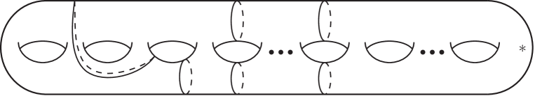
Figure 6: The collection of bounding pairs generating $V(\lambda_{i})\oplus V(\lambda_{i+2})$.

First, for all $i\leq g-2$, we show that $\tau_{i}(H_{i}(\mathcal{I}_{g,*}))$ contains $V(\lambda_{i})\oplus V(\lambda_{i+2})$. Consider the collection of bounding pairs displayed in Figure 6. Let $\sigma\in H_{i}(\mathcal{I}_{g,*})$ be the associated abelian cycle; by Theorem 3.4 we have

$$\tau_{i}(\sigma)=a_{1}\wedge b_{1}\wedge a_{3}\wedge\cdots\wedge a_{i+2}.$$

Recall that there is an $\operatorname{Sp}$–equivariant contraction $C_{k}\colon\textstyle{\bigwedge}^{k}H\to\textstyle{\bigwedge}^{k-2}H$, which was defined in (5). We claim that $\tau_{i}(\sigma)\in\textstyle{\bigwedge}^{i+2}H$ generates $\ker C_{i}\circ C_{i+2}$ as a module. As previously noted, $\ker C_{k}\approx V(\lambda_{k})$ and thus $\ker C_{i}\circ C_{i+2}\approx V(\lambda_{i})\oplus V(\lambda_{i+2})$, so this will verify this case of the theorem.

First note that $\tau_{i}(\sigma)$ is contained in $\ker C_{i}\circ C_{i+2}$; indeed, we have $C_{i+2}(\tau_{i}(\sigma))=a_{3}\wedge\cdots\wedge a_{i+2}$, which lies in $\ker C_{i}$. In particular, we see that $\tau_{i}(\sigma)$ is not contained in $\ker C_{i+2}\approx V(\lambda_{i+2})$. The element

$$\nu\mathrel{\mathop{:}}\mkern-1.2mu=a_{1}\wedge(b_{1}+a_{2})\wedge a_{3}\wedge\cdots\wedge a_{i+2}$$

is clearly in the $\operatorname{Sp}$–orbit of $\tau_{i}(\sigma)$. Thus $\nu-\tau_{i}(\sigma)=a_{1}\wedge a_{2}\wedge a_{3}\wedge\cdots\wedge a_{i+2}$, which lies in $\ker C_{i+2}\approx V(\lambda_{i+2})$, is in the image of $\tau_{i}$. We conclude that the $\operatorname{Sp}$–span of $\tau_{i}(\sigma)$ is contained in $V(\lambda_{i})\oplus V(\lambda_{i+2})$ and properly contains $V(\lambda_{i+2})$, and thus since the $V(\lambda_{k})$ are irreducible, the $\operatorname{Sp}$–span of $\tau_{i}(\sigma)$ is $V(\lambda_{i})\oplus V(\lambda_{i+2})$.

Note that for $i=g-1$, a similar collection of $g-1$ bounding pairs determines an abelian cycle $\sigma$ so that $\tau_{g-1}(\sigma)=a_{1}\wedge b_{1}\wedge a_{2}\wedge\cdots\wedge a_{g}\in\textstyle{\bigwedge}^{g+1}H$. The contraction $C_{g+1}\colon\textstyle{\bigwedge}^{g+1}H\to\textstyle{\bigwedge}^{g-1}H$ is injective [FH, Theorem 17.11]. The image $C_{g+1}(\tau_{g-1}(\sigma))=a_{2}\wedge\cdots\wedge a_{g}$ clearly generates $V(\lambda_{g-1})$, and so $\tau_{g-1}(H_{g-1}(\mathcal{I}_{g,*}))\supseteq V(\lambda_{g-1})$.

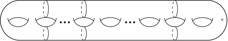
Figure 7: The $i-2$ bounding pairs used to generate $V(\lambda_{i-2})$.

We now show that when $1\leq i\leq g$ and $i$ is even, $\tau_{i}(H_{i}(\mathcal{I}_{g,*}))$ also contains $V(\lambda_{i-2})$. Take the collection of bounding pairs displayed in Figure 7, and let $\sigma\in H_{i-2}(\mathcal{I}_{g,*})$ be the associated abelian cycle; we will consider $\pi^{!}\sigma\in H_{i}(\mathcal{I}_{g,*})$. By Theorem 4.1,

$$\tau_{i}(\pi^{!}\sigma)=2\cdot a_{1}\wedge b_{1}\wedge a_{g}\wedge b_{g}\wedge a_{2}\wedge\cdots\wedge a_{i-2}\wedge a_{g-1}.$$

We claim that this element lies in $\ker C_{i-2}\circ C_{i}\circ C_{i+2}$, but not $\ker C_{i}\circ C_{i+2}$, and thus its $\operatorname{Sp}$–span contains $V(\lambda_{i-2})$ as desired. To see this, note that

$$C_{i+2}(\tau_{i}(\pi^{!}\sigma))=2\cdot(a_{1}\wedge b_{1}+a_{g}\wedge b_{g})\wedge a_{2}\wedge\cdots\wedge a_{i-2}\wedge a_{g-1},$$

so

$$C_{i}\circ C_{i+2}(\tau_{i}(\pi^{!}\sigma))=4\cdot a_{2}\wedge\cdots\wedge a_{i-2}\wedge a_{g-1},$$

which lies in $\ker C_{i-2}$ as claimed.

5.2 Proof of Theorem 1.1

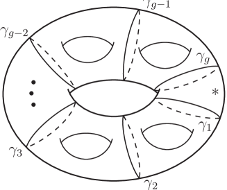
Figure 8: Nonseparating curves; each pair of adjacent curves yields a bounding pair $f_{k}$.

Consider the curves $\gamma_{1},\ldots,\gamma_{g}$ displayed in Figure 8. For $1\leq k<g$, let $f_{k}=T_{\gamma_{k+1}}T_{\gamma_{k}}^{-1}$, and for $2\leq i<g$, let $\sigma\in H_{i}(\mathcal{I}_{g,*})$ be the abelian cycle $\sigma\mathrel{\mathop{:}}\mkern-1.2mu=\{f_{1},\ldots,f_{i}\}$. By Theorem 3.5, $\tau_{i}(\sigma)=0$ since the bounding pairs $f_{k}$ are not truly nested. We will show that $\sigma$ is nontrivial in $H_{i}(\mathcal{I}_{g,*})$, proving the theorem.

Recall Johnson’s map $\tau_{J}\colon\mathcal{I}_{g,*}\to\textstyle{\bigwedge}^{3}H_{\mathbb{Z}}$, which induces

$$(\tau_{J})_{*}\colon H_{i}(\mathcal{I}_{g,*})\to H_{i}(\textstyle{\bigwedge}^{3}H_{\mathbb{Z}})\approx\textstyle{\bigwedge}^{i}(\textstyle{\bigwedge}^{3}H).$$

Let $\iota\colon\mathbb{Z}^{i}\to\mathcal{I}_{g,*}$ be the inclusion of the subgroup $\langle f_{1},\ldots,f_{i}\rangle$. By definition,

$$(\tau_{J})_{*}\sigma=(\tau_{J}\circ\iota)_{*}[\mathbb{Z}^{i}].$$

From the identification of $H_{i}(\textstyle{\bigwedge}^{3}H_{\mathbb{Z}})$ with $\textstyle{\bigwedge}^{i}(\textstyle{\bigwedge}^{3}H)$, we have that

$$(\tau_{J}\circ\iota)_{*}[\mathbb{Z}^{i}]=(\tau_{J})_{*}[f_{1}]\wedge\cdots\wedge(\tau_{J})_{*}[f_{i}].$$

Let $\{a_{1},b_{1},\ldots,a_{g},b_{g}\}$ be a symplectic basis for $H_{1}(S_{g})$ so that $[\gamma_{k}]=a_{g}$ for all ${1\leq k<g}$, and so that $\{a_{k},b_{k}\}$ gives a basis for the homology of the subsurface cut off by $\gamma_{k}$ and $\gamma_{k+1}$ for each $1\leq k<g$. By Johnson’s computation of $\tau_{J}$ (see (9) in Section 2 above), $(\tau_{J})_{*}[f_{k}]=a_{k}\wedge b_{k}\wedge a_{g}$, and thus

$$(\tau_{J})_{*}\sigma=\big{(}a_{1}\wedge b_{1}\wedge a_{g}\big{)}\wedge\cdots\wedge\big{(}a_{i}\wedge b_{i}\wedge a_{g}\big{)}.$$

This element is nonzero in $\textstyle{\bigwedge}^{i}(\textstyle{\bigwedge}^{3}H)$ since $\{a_{k}\wedge b_{k}\wedge a_{g}\}_{k=1}^{i}$ is linearly independent in $\textstyle{\bigwedge}^{3}H$. Thus $\tau_{J}(\sigma)\neq 0$ and so $\sigma\neq 0$, completing the proof of Theorem 1.1.

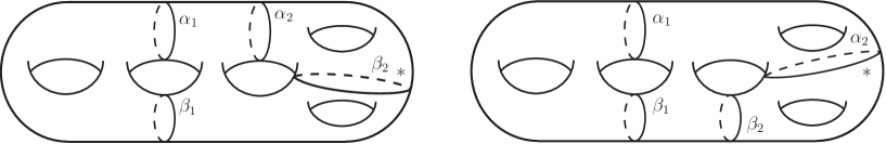
Figure 9: Homologically distinct abelian cycles not distinguishable by $\tau_{i}$.
a. The collection $\{f_{1},f_{2}\}$. b. The collection $\{g_{1},g_{2}\}$.

Remark. We now give another example showing the non-injectivity of $\tau_{i}$. One notable feature of this example is that we replace $\tau_{J}$ in the proof above by the maps $\tau_{i}$ themselves. For even $i\leq g-2$, let $\{f_{k}\}$ and $\{g_{k}\}$ be two truly nested collections of bounding pairs as in Figure 9, so that $f_{k}$ and $g_{k}$ are homologous; the collections cut off the same farthest subsurface; but the closest subsurfaces cut off by $\{f_{k}\}$ and $\{g_{k}\}$ determine different symplectic forms in $\bigwedge^{2}H_{1}(S_{g})$. By Theorem 3.4, $\tau_{i}(\{f_{1},\ldots,f_{i}\})=\tau_{i}(\{g_{1},\ldots,g_{i}\})$. However, Theorem 4.1 shows that $\pi^{!}(\{f_{1},\ldots,f_{i}\})$ is not equal to $\pi^{!}(\{g_{1},\ldots,g_{i}\})$, and thus $\{f_{1},\ldots,f_{i}\}$ is not equal to $\{g_{1},\ldots,g_{i}\}$ in $H_{i}(\mathcal{I}_{g,*})$. Finally, note that we may choose $\{f_{i}\}$ and $\{g_{i}\}$ so that $(\tau_{J})_{*}\{f_{1},\ldots,f_{i}\}=(\tau_{J})_{*}\{g_{1},\ldots,g_{i}\}$, so this method yields new elements of $\ker\tau_{i}$ which cannot be detected by $(\tau_{J})_{*}$.

5.3 Detecting homology using $\tau_{J}$

In general, computing the image of $(\tau_{J})_{*}$ is very difficult; in particular, by work of Kawazumi–Morita (see [Mo99, §6.4]), a complete solution would resolve the long-standing question of whether the even Morita–Mumford–Miller classes $e_{2i}\in H^{4i}(\mathcal{I}_{g,*})$ are nontrivial. However, in the lowest dimensions, the images have been found explicitly for the related case of closed surfaces. Considering the map

$$(\tau_{J})_{*}\colon H_{2}(\mathcal{I}_{g})\to\textstyle{\bigwedge}^{2}\big{(}\textstyle{\bigwedge}^{3}H/H\big{)},$$

Hain [Ha97] found that for $g\geq 6$, the image of $(\tau_{J})_{*}$ is isomorphic to

$$V(\lambda_{6})\oplus V(\lambda_{4})\oplus V(\lambda_{2})\oplus V(\lambda_{2}+\lambda_{4}).$$

Similarly, Sakasai [Sa] found that, up to possibly a factor of $V(\lambda_{1})=H$, the image of

$$(\tau_{J})_{*}\colon H_{3}(\mathcal{I}_{g})\to\textstyle{\bigwedge}^{3}(\textstyle{\bigwedge}^{3}H/H)$$

for $g\geq 9$ is isomorphic to

$$V(\lambda_{5}+2\lambda_{2})\oplus V(2\lambda_{4}+\lambda_{1})\oplus V(\lambda_{6}+\lambda_{3})\oplus V(\lambda_{4}+\lambda_{3})$$

$$\oplus V(\lambda_{7}+\lambda_{2})\oplus V(\lambda_{5}+\lambda_{2})\oplus V(\lambda_{3}+\lambda_{2})\oplus V(\lambda_{6}+\lambda_{1})\oplus V(\lambda_{4}+\lambda_{1})$$

$$\oplus V(\lambda_{9})\oplus V(\lambda_{7})\oplus V(\lambda_{5})\oplus V(\lambda_{5})\oplus V(\lambda_{3}).$$

The stability of these decompositions is exactly the behavior predicted by Conjecture 1.6. Hain and Sakasai also compute the decompositions for smaller $g$, but they do not stabilize until $g\geq 6$ and $g\geq 9$ respectively.

Department of Mathematics
University of Chicago
5734 University Ave.
Chicago, IL 60637
E-mail: tchurch@math.uchicago.edu, farb@math.uchicago.edu

References

[BBM] M. Bestvina, Kai-Uwe Bux, and D. Margalit, The
dimension of the Torelli group, Journal Amer. Math. Soc. 23 (2010), no. 1, 61–105.
[BMS] H. Bass, J. Milnor, and J.P. Serre, Solution of the
congruence subgroup problem for and , Publ. Math. IHES, No. 33 (1967),
59–137.
[Bi] J. Birman, On Siegel’s modular group, Math. Ann. 191 (1971), 59–68.
[BD] S. Boldsen and M. Dollerup, Towards representation stability for the second homology of the Torelli group, arXiv:1101.5767v2, February 2011.
[Bo] A. Borel, Density properties for certain subgroups of
semi-simple groups without compact components, Ann. of Math.
(2) 72 (1960), 179–188.
[CF] T. Church and B. Farb, Homological stability and representation theory, arXiv:1008.1368,
August 2010.
[Co] P. Conner, Differentiable Periodic Maps, second edition, Lecture Notes in Mathematics 738, Springer, Berlin, 1979.
[FH] W. Fulton and J. Harris, Representation theory. A
first course, Graduate Texts in Mathematics 129, Readings in
Mathematics, Springer-Verlag, New York, 1991.
[FM] B. Farb and D. Margalit, A primer on mapping class groups, to appear in Princeton Mathematical Series, Princeton University Press. Available at:http://www.math.utah.edu/~margalit/primer/
[Ha95] R. Hain, Torelli groups and geometry of moduli
spaces of curves, in Current topics in complex algebraic
geometry (Berkeley, CA, 1992/93), 97–143, Math. Sci. Res. Inst. Publ.,
Vol. 28, 1995.
[Ha97] R. Hain, Infinitesimal presentations of the
Torelli groups, J. Amer. Math. Soc. 10 (1997), no. 3, 597–651.
[HL] R. Hain and E. Looijenga, Mapping class groups and
moduli spaces of curves, in Algebraic geometry—Santa Cruz 1995, 97–142,
Proc. Sympos. Pure Math., 62, Part 2, Amer. Math. Soc.,
Providence, RI, 1997.
[HM] A. Hatcher and D. Margalit, Generating the Torelli group, preprint (2011).
[KM] N. Kawazumi and S. Morita, The primary approximation
to the cohomology of the moduli space of curves and cocycles for the
Mumford-Morita-Miller classes, preprint.
[Jo79] D. Johnson, Homeomorphisms of a surface which act trivially on homology,
Proc. Amer. Math. Soc. 75 (1979), no. 1, 119–125.
[Jo80] D. Johnson, An abelian quotient of the mapping
class group , Math. Ann. 249 1980 3, 225–242.
[Jo83] D. Johnson, A survey of the Torelli
group. In Low-dimensional topology (San Francisco,
Calif., 1981), volume 20 of Contemp. Math., pages
165–179. Amer. Math. Soc., 1983.
[Ma] G. Margulis, Discrete Subgroups of Semisimple Lie
Groups, Ergebnisse der Math. 17, Springer-Verlag, 1991.
[Me] G. Mess, The Torelli groups for genus and surfaces.
Topology 31 (1992), no. 4, 775–790.
[Mo89] S. Morita, On the structure and the homology of the
Torelli group, Proc. Japan Acad. Ser. A Math. Sci. 65
(1989), no. 5, 147–150.
[Mo99] S. Morita, Structure of the mapping class groups of
surfaces: a survey and a prospect. Proceedings of the Kirbyfest
(Berkeley, CA, 1998), 349–406, Geom. Topol. Monogr. 2, 1999.
[Mo01] S. Morita, Geometry of Characteristic Classes,
Transl. of Math. Monog., 199. Amer. Math. Soc., 2001.
[MW] I. Madsen and M. Weiss, The stable moduli space of
Riemann surfaces: Mumford’s conjecture, Ann. of Math. 165
(2007) 3, 843–941.
[Po] J. Powell, Two theorems on the mapping class group of a surface, Proc. Amer. Math. Soc. 68 (1978), no. 3, 347–350.
[Sa] T. Sakasai, The Johnson homomorphism and the third
rational cohomology group of the Torelli group, Topology and
its Applications 148 (2005), 83–111.
[Th]
R. Thom, Quelques propriétés globales des variétés différentiables,
Comment. Math. Helv. 28 (1954), 17–86.