Particle Swarm Optimization and gravitational wave data analysis: Performance on a binary inspiral testbed

Abstract

The detection and estimation of gravitational wave (GW) signals belonging to a parameterized family of waveforms requires, in general, the numerical maximization of a data-dependent function of the signal parameters. Due to noise in the data, the function to be maximized is often highly multi-modal with numerous local maxima. Searching for the global maximum then becomes computationally expensive, which in turn can limit the scientific scope of the search. Stochastic optimization is one possible approach to reducing computational costs in such applications. We report results from a first investigation of the Particle Swarm Optimization (PSO) method in this context. The method is applied to a testbed motivated by the problem of detection and estimation of a binary inspiral signal. Our results show that PSO works well in the presence of high multi-modality, making it a viable candidate method for further applications in GW data analysis.

I Introduction

The detection and estimation of a gravitational wave (GW) signal belonging to a parameterized family of waveforms requires, in general, the numerical maximization of some data-dependent function over the space of the signal parameters. For example, in the matched filtering helstrom ; wainstein+zubakov method, which is the focus of this paper, the function to be maximized is a suitably defined inner product between the data and parameterized signal waveforms. The global maximum of this function serves as a detection statistic. A point estimate of the signal parameters is furnished by the location of the global maximum in parameter space.

The presence of noise in the output of GW detectors leads to a large number of local maxima in this function that are distributed randomly in parameter space. The search for the global maximum in this forest of local maxima then becomes a computationally expensive task. This can affect the sensitivity of a search by limiting either the volume that is searched in parameter space or the integration length of data required for accumulating sufficient signal-to-noise ratio (SNR), or both. The computational efficiency of the search for the global maximum is, thus, an important issue in GW data analysis. The various search strategies proposed in the GW literature so far can be broadly divided into those based on sampling the function on predetermined grids of points in parameter space owen96 ; owen99 ; mohanty+dhurandhar:96 , and those that use stochastic optimization methods (e.g., christensen04 ; cornish+crowder:2005 ; wickham+etal:2006 ).

In the class of grid-based methods, significant savings in computational costs have been demonstrated with a hierarchy of grids mohanty+dhurandhar:96 ; mohanty98 ; sengupta+etal . A nice feature of grid-based methods is that they are easy to characterize statistically and, hence, design variables of the algorithm, such as the spacing of points, can be fixed systematically.

Stochastic methods do not use pre-determined grids but employ some form of random walk through the parameter space. The probabilistic rules of the random walk are tuned to maximize the chances of its terminating close to the global maximum. There are many algorithms that fall under the class of stochastic methods, a hybrid of simulated annealing and Metropolis-Hastings Markov Chain Monte Carlo (MCMC) being the most widely explored in GW data analysis christensen04 ; cornish+crowder:2005 ; wickham+etal:2006 .

Since the number of points in a grid grows exponentially with the dimensionality of the parameter space, stochastic methods tend to outperform grid-based ones with an increase in the number of signal parameters. It is worth noting here that stochastic methods in GW data analysis incur the additional computational cost of generating signal waveforms on the fly. In grid-based methods, on the other hand, waveforms can be computed and stored in advance of processing the data. Stochastic methods can, therefore, lose their advantage if the computational cost of generating waveforms becomes too high.

The performance of a stochastic method may be sensitive to the values to which its design variables are tuned. Since the tuning is usually done on simulated data, it is not clear how robust current stochastic methods are against features of real data such as non-stationarity and non-Gaussianity. Additionally, the number of design variables that require careful tuning is fairly large for some of the methods. In such cases, tuning becomes more of an art than a well defined procedure and this may also affect robustness. In some methods, prior information is used about generic features of the function to be maximized. This may not be reliable if the assumptions behind the prior information, such as a particular noise model, become invalid. To properly address issues such as these it is important that a wide variety of stochastic methods be explored in GW data analysis .

Particle Swarm Optimization (PSO) kennedy95 , first proposed by Kennedy and Eberhardt in 1995, is a stochastic method that has been garnering a lot of attention recently in many application areas proc:SIS09 . An attractive feature of PSO is that, in its basic form, it has a small number of design variables. On standard testbeds, PSO has been found to have comparable or superior performance to other well known methods such as MCMC.

This paper presents the first application of PSO to GW data analysis. We pose the following specific questions:

1. Is PSO a viable method when applied to a function that is highly multi-modal and essentially stochastic in nature? This is the typical case in GW data analysis.

2. How many design variables are there in PSO, and how many of them need to be tuned well?

3. Can the tuning of these variables be done without requiring prior information about features of the function, thus increasing the robustness of the method?

4. What is the computational cost of the method and what are the most important technical improvements required for the future?

To answer these questions in the most direct and reliable manner, we construct a testbed based on the well understood task of detecting and estimating binary inspiral signals in data from a single ground-based detector. This problem involves low-dimensionality but offers the more serious challenge of high multi-modality. To keep the focus on the latter, a simplification is made regarding the shape of the search region such that it admits unphysical waveforms. Thus, the implementation of PSO presented here is not directly applicable to binary inspiral searches at present. The required technical refinements are discussed in the paper. In addition, a novel and systematic tuning procedure is introduced that is based on data containing only noise. This procedure may be useful for other stochastic methods also.

The rest of the paper is organized as follows. Sec. II describes the testbed and Sec. III describes the PSO method. We explain our procedure for tuning the design variables of PSO in Sec. IV. Sec. V then presents results from numerical simulations. Our conclusions and pointers to future work are presented in Sec VI.

Notation

${\bf x}$, ${\bf y}$, etc: A time series with a finite number, $N$, of samples. The $k^{\rm th}$ sample, $0\leq k\leq N-1$, is denoted by $x[k]$.

$\delta_{s}$, $T$: The sampling interval and the duration of ${\bf x}$ respectively. The number of samples in ${\bf x}$ is $N=[T/\delta_{s}]$, where the square brackets denote truncation to the nearest integer.

$\Theta$ : The set of parameters describing a family of signals.

${\bf s}(\Theta)$: The time series of the signal corresponding to parameter values $\Theta$. The $k^{\rm th}$ sample of ${\bf s}(\Theta)$ is denoted by $s[k;\Theta]$. In our case, signals have a well-defined start and stop time and the interval between them may be less than $T$. However, ${\bf s}(\Theta)$ still consists of $N$ samples with the samples outside the interval enclosed by the start and stop times set to 0 (zero-padding).

$\widetilde{\bf x}$: The Discrete Fourier Transform (DFT) of ${\bf x}$. The DFT value at the frequency $k/T$, $k=0,1,\ldots,[N/2+1]$, is denoted as $\widetilde{x}[k]$. The DFT of ${\bf s}(\Theta)$ is denoted by $\widetilde{\bf s}(\Theta)$ and its value at the $k^{\rm th}$ frequency by $\widetilde{s}[k;\Theta]$.

$\langle{\bf x},{\bf y}\rangle$: The time series introduced above are elements of $\mathbb{R}^{N}$, the vector space of real $N$-tuples. From the point of view of detection and estimation of a signal in data with additive stationary noise, a natural inner product can be introduced on this vector space,

$$\langle{\bf x},{\bf y}\rangle=4\mathcal{R}\left(\sum_{k=0}^{[N/2+1]}{\frac{\widetilde{x}^{*}[k]\widetilde{y}[k]}{S_{n}[k]T}}\right)$$ (1)

where $S_{n}[k]$ is the one-sided Power Spectral Density (PSD) of the noise.

$\|{\bf y}\|$: the norm on $\mathbb{R}^{N}$,

$$\|{\bf y}\|^{2}=\langle{\bf y},{\bf y}\rangle\;,$$ (2)

induced by the inner product defined above. The signal to noise ratio (SNR) of a signal ${\bf s}(\Theta)$ is defined as $\|{\bf s}(\Theta)\|$.

II Test bed

In this section, we describe the testbed to which PSO is applied. The testbed is constituted by the noise model, signal family and the function to be maximized.

II.1 Noise model

A GW signal incident on an interferometric ground-based detector produces a difference in the lengths of its two arms. After calibrating out the common arm length and the transfer function of the detector, the data, ${\bf x}$, contains the measured GW-induced strain added to instrumental and environmental noise ${\bf n}$. Thus, ${\bf x}={\bf n}$ when no GW signal is present, and ${\bf x}={\bf s}(\Theta)+{\bf n}$ when there is. In our simulations, ${\bf n}$ is a realization of a stationary, Gaussian noise process with a PSD, $S_{n}[k]$, that matches the initial LIGO ligo design sensitivity curve in shape ifo_sensitivity .

II.2 Signal waveforms

We use the signal family associated with a non-spinning inspiraling binary system, computed up to the second post-Newtonian (2PN) order blanchet+etal . This system consists of two non-spinning compact stars (Neutron Stars or Black Holes) losing orbital binding energy through GW emission. Members of this signal family have chirp waveforms with monotonically increasing instantaneous amplitude and frequency.

For the case of a single detector, the parameters specifying the 2PN signal waveforms can be grouped into two sets. The first set is that of the chirp-time bss:chirptimes parameters, $\{\tau_{a}\}$, $a=0,1,1.5,2$, that are constructed out of the masses of the two components of the binary. Expressions for the chirp-time parameters are provided in Appendix A. The second set consists of the time-of-arrival, $t_{a}$, the initial phase, $\Phi_{a}$ and the amplitude, $\mathcal{A}$. Interferometric ground-based detectors have a sharp rise in seismic noise below some frequency $f_{a}$ ( $=40$ Hz for inital LIGO). The chirp signal from a binary inspiral is essentially unobservable when its instantaneous frequency is below $f_{a}$. The time at which the signal becomes visible is $t_{a}$ and the corresponding instantaneous phase of the signal is $\Phi_{a}$.

Since all the four chirp-times depend on the masses of the two compact stars, only two of them are independent. We choose $\tau_{0}$ and $\tau_{1.5}$ as the two independent chirp-time parameters. Thus, the set of signal parameters is $\Theta=\{\mathcal{A},\Phi_{a},t_{a},\theta=\{\tau_{0},\tau_{1.5}\}\}$.

As discussed in Sec. I, the computational cost of generating waveforms on the fly is important for stochastic methods like PSO. The 2PN signal family is amenable to a fast implementation because a sufficiently accurate analytical form exists for the Fourier transform of these waveforms droz+etal ,

$$\widetilde{s}[k;\Theta] = \left\{\begin{array}[]{ll}0\;,&k\leq[f_{a}T]\;,\\ \mathcal{A}\mathcal{N}f^{-7/6}\exp\left[-2\pi ift_{a}+i\Phi_{a}-i\psi(f;\theta)+i\frac{\pi}{4}\right]\;,&[f_{a}T]<k\leq[f_{c}T]\;,\\ 0\;,&k>[f_{c}T]\end{array}\right.$$ (6)

where, the lower cutoff frequency $f_{a}$ was explained above and the upper cutoff frequency $f_{c}$ follows from the termination of the inspiral waveform when the binary reaches its last stable orbit. For our testbed, we set $f_{c}=700$ Hz although in a real search it depends on the mass of the binary system. The expression for $\psi(f;\theta)$ is given in Appendix A. The normalization constant $\mathcal{N}$ is defined such that, $\|{\bf s}(\{\mathcal{A}=1,\Phi_{a},t_{a},\theta\})\|^{2}=1$. It follows that $\mathcal{A}$ is the SNR of the signal.

Later on, we use the fact that although not all values of $\theta$ correspond to valid binary mass components, Eq. 6 can still be used to generate perfectly normal waveforms. These waveforms are also chirps but their phase evolution does not correspond to any physical binary system.

II.3 Fitness function

The function to be maximized is,

$$\Lambda(t_{a},\theta|{\bf x}) = \left[\langle{\bf q}_{0}(t_{a},\theta),{\bf x}\rangle^{2}+\right.$$ (7)

$$\left.\langle{\bf q}_{\pi/2}(t_{a},\theta),{\bf x}\rangle^{2}\right]^{1/2}\;,$$

$${\bf q}_{\phi}(t_{a},\theta) = {\bf s}(\{\mathcal{A}=1,\Phi_{a}=\phi,t_{a},\theta\})\;.$$ (8)

This function is obtained by maximizing the log-likelihood, $\langle{\bf x},{\bf s}(\Theta)\rangle-(1/2)\|{\bf s}(\Theta)\|^{2}$ analytically over $\mathcal{A}$ and $\Phi_{a}$.

For given $\theta$, the evaluation of $\langle{\bf q}_{\phi}(t_{a},\theta),{\bf x}\rangle$ over $t_{a}=m\delta_{s}$, $m=0,1,\ldots,N-1$, is a cross-correlation operation that can be computed efficiently using the Fast Fourier Transform (FFT). Thus, the function that is maximized using PSO is,

$$\lambda(\theta|{\bf x})=\max_{t_{a}}\Lambda(t_{a},\theta|{\bf x})\;.$$ (9)

In the remainder of the paper, $\lambda(\theta|{\bf x})$ will be called the fitness function in keeping with the standard terminology used in much of the literature on stochastic methods.

The presence of noise in ${\bf x}$ makes the fitness function highly multi-modal as shown in Fig 1. The large number of local maxima with random locations and sizes poses a strong challenge to stochastic methods. When the noise is stationary and Gaussian, and the signal present in the data is from the waveform family that one is searching for, certain characteristic features are present in the fitness function. For example, the shape of the peak in Fig. 1 is elongated on the average along a predictable direction. MCMC methods in the GW literature use this type of prior information about the fitness function in tuning the design variables cornish+crowder:2005 .

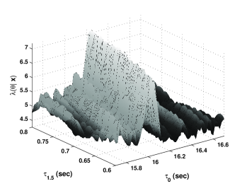
Figure 1: A realization of the fitness function for the binary inspiral testbed. The data contains a signal with an SNR=8.0. In the absence of noise, the fitness function has only one extremum at the location identified by the chirp-times of the signal. The presence of noise leads to a forest of local maxima.

III Particle Swarm Optimization

The PSO algorithm is first described in terms of a general fitness function $\lambda(\theta)$, over some parameter set $\theta$. Later, we specialize the discussion to the case of the binary inspiral testbed.

III.1 The PSO Algorithm

Let $\theta=\{\theta_{1},\theta_{2},\ldots,\theta_{D}\}$ denote a point in $\mathbb{R}^{D}$, and $\lambda(\theta)$ be the fitness function. The essential idea behind PSO is to compute $\lambda(\theta)$ simultaneously at several locations and use these samples to influence the locations for computing the next set of samples. This process continues iteratively until some stopping rule is satisfied. The process can be visualized by treating the sample locations as a swarm of particles that moves in $\mathbb{R}^{D}$, hence the name of the algorithm. A precise description now follows.

Let the coordinates in $\mathbb{R}^{D}$ of the $i^{\rm th}$ particle in a swarm of $N_{p}$ particles be $Q_{i}[k]$ at the $k^{\rm th}$ step in the search $(k=0,1,\ldots$). Associated with this particle is a velocity vector $V_{i}[k]$ that determines $Q_{i}[k+1]$,

$$Q_{i}[k+1] = Q_{i}[k]+V_{i}[k]\;.$$ (10)

The PSO algorithm is usually started with randomly chosen particle locations and velocities. In our implementation, we position the particles initially on a regular grid while the initial velocities are kept random.

Let the maximum value of $\lambda(\theta)$ found by the $i^{\rm th}$ particle over $k$ steps be $R_{i}(k)$ and the location of $R_{i}(k)$, called the particle’s best location pbest, be $P_{i}[k]$. Thus,

$$R_{i}(k)=\lambda(P_{i}[k])\geq\lambda(Q_{i}[j]);\;j\leq k\;.$$ (11)

Let the maximum over $\{R_{i}(k)\}$, $i=1,\ldots,N_{p}$, be $R_{g}(k)$ and its location, called the global best location gbest be $P_{g}[k]$,

$$R_{g}(k)=\lambda(P_{g}[k])\geq\lambda(P_{j}[k]);\;\forall j\;.$$ (12)

At any step, there is always one particle in the swarm whose pbest is also the gbest. We call this particle the best particle at step $k$. Note that both pbest and gbest are locations found over the entire past history of the motion of the particles. They need not necessarily change at every step.

The velocity for the $i^{\rm th}$ particle at the next step, $k+1$, is determined by the dynamical equation,

$$V_{i}[k+1] = wV_{i}[k]+c_{1}\chi_{1}(P_{i}[k]-Q_{i}[k])+$$ (13)

$$c_{2}\chi_{2}(P_{g}[k]-Q_{i}[k])\;,$$

where $w$, which can depend on $k$, is called the inertia weight, $c_{1}$ and $c_{2}$ are called acceleration constants, and $\chi_{1}$, $\chi_{2}$ are random numbers drawn independently at each step from the uniform distribution on $[0,1]$.

Finally, for any component $V_{i,m}[p]$ of the particle velocity $V_{i}[p]=(V_{i,1}[p],\ldots,V_{i,D}[p])$,

$$V_{i,m}[p]=\left\{\begin{array}[]{cc}V_{{\rm max},m}\;,&V_{i,m}[p]>V_{{\rm max},m}\\ -V_{{\rm max},m}\;,&V_{i,m}[p]<-V_{{\rm max},m}\end{array}\right.\;,$$ (14)

where $V_{{\rm max},k}>0$, $k=1,\ldots,D$, and $V_{\rm max}=(V_{{\rm max},1},\ldots,V_{{\rm max},D})$ is called the maximum velocity.

Like all stochastic methods, PSO involves a competition between wide ranging exploration of the fitness function and convergence to a best value. In order to avoid trapping by a local maximum, the method must be able to explore other parts of the parameter space, while to find the global maximum, the method must eventually explore a progressively smaller region around some point. The way this competition is implemented in the PSO algorithm is seen clearly from Eqs. 13. The first term simply moves a particle along a straight line, while the remaining two terms are sources of acceleration, one pulling it towards its pbest and another pulling it towards gbest. The last two effects are combined with random weights $\chi_{1}$ and $\chi_{2}$. The random deflections and inertial motion allow a particle to explore the fitness function, while the attractive pulls of pbest and gbest counter this behavior. With a dynamic inertia weight that decreases in time, the attractive pull eventually wins over. A rudimentary emulation of real biological swarming behavior is built in through each particle being aware of gbest.

The PSO algorithm has another interesting feature. The best particle, by definition, has its pbest $P_{i}[k]$ coincident with gbest, $P_{g}[k]$, making the terms $P_{i}[k]-Q_{i}[k]$ and $P_{g}[k]-Q_{i}[k]$ equal for it. This particle then accelerates towards gbest alone and only moves along a straight line through this location. This situation continues until a new gbest is found. In effect, one particle at any step shows a convergence behavior, exploring the neighborhood of the current gbest, while the other particles continue their exploration.

III.2 Termination criterion

For stochastic methods, the probability of convergence to the global maximum is usually guaranteed only in the asymptotic limit. Hence, any practical implementation of a stochastic method must include a criterion for terminating the search. The criterion we adopt for termination is specific to the fitness function for the binary inspiral testbed and, accordingly, $\theta$ now refers to the chirp time parameters.

If the particles in PSO continue to move over several steps but do not find a significantly different gbest, it is likely that the current gbest lies close to the global maximum. A natural criterion for termination then is to check if gbest stays confined to a small region over a predetermined number of steps.

When the data contains only a signal, ${\bf x}={\bf s}(\{\mathcal{A},\Phi_{a},t_{a},\theta\})$, the fitness function is maximum at the location $\theta$ of the signal. ( ${\bf s}(\theta)\equiv{\bf s}(\{\mathcal{A},\Phi_{a},t_{a},\theta\})$ for brevity in the following since the other parameters do not figure in the fitness function.) The fractional drop in the fitness function for a small displacement $\Delta\theta=(\Delta\theta_{1}=\Delta\tau_{0},\Delta\theta_{2}=\Delta\tau_{1.5})$ is given by,

$$1-\frac{\lambda(\theta+\Delta\theta|{\bf s}(\theta))}{\lambda(\theta|{\bf s}(\theta))} \simeq \frac{-\sum_{i,j=1}^{2}{\cal H}_{ij}\Delta\theta_{i}\Delta\theta_{j}}{2\lambda(\theta|{\bf s}(\theta))}\;,$$ (15)

$${\cal H}_{ij} = \left.\frac{\partial^{2}\lambda(\theta^{\prime}|{\bf s}(\theta))}{\partial\theta_{i}^{\prime}\partial\theta_{j}^{\prime}}\right|_{\theta^{\prime}=\theta}\;,$$ (16)

where $\theta$ is the location of the signal. For a small fractional drop $\alpha$, therefore, we get an ellipsoidal region $\mathcal{S}_{\alpha}(\theta)$ centered at $\theta$ such that $\lambda(\theta^{\prime}|{\bf s}(\theta))\geq(1-\alpha)\lambda(\theta|{\bf s}(\theta))$ if $\theta^{\prime}\in\mathcal{S}_{\alpha}(\theta)$.

Now, the neighborhood of the global maximum in the presence of noise is also $S_{\alpha}(\theta)$ on the average for a fractional drop $\alpha$. Therefore, it is natural to choose the region of convergence to be $\mathcal{S}_{\alpha}(\theta)$ in general. This reduces the task of specifying the region to simply choosing a value for $\alpha$. Following a convention widely used in the GW literature owen96 , we fix $\alpha=0.03$.

Thus, we arrive at the following criterion for terminating PSO. At each step $k$, (i) obtain the ellipsoid around gbest, that is, $\mathcal{S}_{\alpha}(P_{g}[k])$. (ii) If the best location $P_{g}[k+1]$ falls outside $\mathcal{S}_{\alpha}(P_{g}[k])$, then reset the region of convergence to the new best location, i.e., use $\mathcal{S}_{\alpha}(P_{g}[k+1])$. (iii) If the region of convergence is not found to change over $N_{t}$ successive steps, then terminate PSO.

The termination criterion implies that if PSO terminates near the true global maximum, the fitness value found will have a fractional drop less than $\alpha$. Consequently, it will have a performance comparable to a grid-based search in which the templates are spaced according to the minimal match criterion owen99 and the minimal match is $1-\alpha$. This is important for situations where a grid-based search is infeasible as it guarantees that PSO will perform as well or better. The probability of convergence to the global maximum must be high, however, and this is the objective of the tuning process described later.

III.3 Search Boundary

Even with the termination criterion in place, the search region must be finite in order for PSO to terminate in a finite number of steps. Otherwise, the swarm may continue to find a better gbest and the termination criterion may never be satisfied. This is especially relevant in the case when the data has only noise. Thus, the PSO dynamics must be supplemented with appropriate boundary conditions. Many approaches to this problem have been proposed, with a good summary provided in boundaryConditions . In this paper, we use the invisible wall boundary condition, but we also briefly describe some of the others below.

III.3.1 Types of boundary conditions

The boundary conditions proposed in the PSO literature are as follows. (This list is taken from boundaryConditions and is by no means an exhaustive one.)

Absorbing walls – When a particle crosses a rectangular boundary, the velocity component perpendicular to the boundary is zeroed. Eventually, this allows the particle to be pulled into the search domain.

Reflecting walls – As with the absorbing walls condition, the particle velocity is altered but instead of being zeroed, the velocity component perpendicular to the wall is reversed in sign. This throws the particle back into the search domain.

Invisible walls – No change is made to the dynamics of the boundary crossing particle but $\lambda(\theta|{\bf x})$ is set to zero and it is not evaluated as long as the particle stays outside the boundary.

We have tried all three boundary conditions but, like the authors of boundaryConditions , we find that the invisible wall condition tends to perform better than the other two.

III.3.2 Search region for the testbed

The simplest search region in $\theta$ parameter space is a rectangle $\tau_{0,min}\leq\tau_{0}\leq\tau_{0,max}$ and $\tau_{1.5,min}\leq\tau_{1.5}\leq\tau_{1.5,max}$. A part of this region, however, admits waveforms that do not correspond to a physically valid binary system. This is due to the dependence of $\tau_{0}$, $\tau_{1.5}$ on the symmetric combinations of binary component masses $M$ and $\mu$, the total and reduced mass of the binary respectively, and the inequality $M\geq 4\mu$. Nonetheless, as remarked in Sec. II.2, there is no technical problem in generating waveforms corresponding to the unphysical chirp times and nothing strange happens to the fitness function there. See Fig. 1, for example, where a part of the parameter region shown is unphysical. Since the primary utility of the binary inspiral problem in this paper is to provide a testbed for PSO, this physical constraint is ignored.

The rectangular search region allows the coordinate transformation,

$$x_{1} = (\tau_{0}-\tau_{0,min})/(\tau_{0,max}-\tau_{0,min})\;,$$ (17)

$$x_{2} = (\tau_{1.5}-\tau_{1.5,min})/(\tau_{1.5,max}-\tau_{1.5,min})\;,$$ (18)

such that $x_{i}\in[0,1]$, $i=1,2$. In our codes, all PSO equations use $x_{1}$ and $x_{2}$ and the corresponding velocity components.

We choose $\tau_{0,min}=0.94$ sec, $\tau_{0,max}=37.48$ sec, $\tau_{1.5,min}=0.234$ sec and $\tau_{1.5,max}=1.021$ sec. With $\tau_{0}$ and $\tau_{1.5}$ along the horizontal and vertical axes respectively, the upper right hand corner corresponds to binary component masses (in $M_{\odot}$) $m_{1}=1.1$ and $m_{2}=1.1$. The lower left hand corner corresponds to $m_{1}=10.5$ and $m_{2}=9.7$.

III.4 PSO design variables

One of the questions posed at the beginning was about the number of design variables in PSO. In our implementation, there are a total of 9 that are listed below for reference.

$N_{p}$: Number of particles in the swarm.

$c_{1},\,c_{2}$: Acceleration constants.

$V_{max}$: Maximum velocity of a particle.

$\alpha,\,N_{t}$: The parameters used to specify the termination criterion for PSO. These parameters are not part of the standard PSO algorithm.

Parameters governing the inertia decay law: The inertia weight is decreased in value as PSO progresses through a search. The PSO literature is full of different types of decay laws but, in general, it is known that a strictly linear decay law is not very useful. We have developed the following decay law that has elements of both linearity and non-linearity. Let $w[k]$ be the value of the inertia weight at step $k$,

$$w[k]=w_{0}-m(k-k_{0})/N_{t}\;,$$ (19)

where $w_{0}>0$ and $m>0$. The parameter $k_{0}$ starts with an initial value of $k_{0}=0$ and is kept fixed as long as gbest stays within the current region of convergence. If gbest exits the convergence region at some step $k^{\prime}$ without termination, $k_{0}$ is set equal to $k^{\prime}$. Thus, the value of the inertia is reset to the starting value of $w_{0}$ every time termination fails and the linear decay of the inertia starts anew.

$N_{rep}$: For given data ${\bf x}$, independent runs of PSO yield different values of $\lambda(\theta|{\bf x})$ corresponding to the different fitness values at termination. This is unavoidable for any stochastic method. However, termination near the true global maximum in independent runs of PSO on the same data should result in the clustering of the different values found and their locations. We can turn this argument around by running PSO independently several times on the same data and using the formation of a cluster as an indicator of successful termination in the vicinity of the global maximum. The number of independent runs of PSO on the same data, $N_{rep}$, is also a design variable.

IV Tuning the design variables

For any stochastic method, convergence to the global maximum can only be quantified as a probability. In some asymptotic limit, such as particle number $N_{p}\rightarrow\infty$ for PSO, this probability becomes unity. However, this also implies an infinitely large computing cost. Thus the design variables must be tuned to find the best trade-off between the probability of convergence and the associated computational cost. We present here the procedure followed for tuning the design variables of PSO.

In contrast to the tuning procedure used for most MCMC methods in the GW literature, our approach is not based on data containing a signal but data that is purely noise. The latter is the worst case scenario for any stochastic method. However, good performance in the pure noise case more or less guarantees success when a signal is present. Moreover, this approach to tuning avoids any bias due to the use of a particular set of signals or SNRs.

The tuning procedure presented here can be used, in principle, to tune all the nine design variables of PSO (c.f., Sec. III.4). However, applying the procedure to all of them is computationally too expensive, at least for the objectives of this paper. We focus instead on two of the most important variables for the performance of PSO, $N_{p}$ and $N_{t}$. For the rest, we either choose values commonly used in the literature or simply pick reasonable ones based on our experience with PSO. Thus, we set : $c_{1}=c_{2}=2$, $V_{max}=(0.5,0.5)$, $w_{0}=0.9$, $m=0.4$, $\alpha=0.03$ and $N_{rep}=5$.

IV.1 Criterion for optimal tuning

Measuring the probability of convergence for the pure noise case presents a practical problem. In simulations where a large SNR signal is present, we know that the true maximum is most likely to be in close proximity to the location of the signal and it can be found reliably using, say, a small area grid-based search. For the pure noise case, however, the location is not known a priori, even approximately, and the only reliable solution is a grid-based search over the entire search region. However, we avoid this solution because (i) the simulations become computationally very expensive, and more importantly, (ii) it would fail for higher dimensional problems where grid-based searches are infeasible.

To circumvent this problem, we invoke the argument outlined in Sec. III.4 for using $N_{rep}$ wherein termination in the vicinity of the global maximum is indicated by the clustering of the fitness and parameter values over independent runs of PSO. One way to further confirm the association between a cluster and the global maximum is to increase the number of particles significantly and verify that a cluster forms around the same location. This is similar to what is done, for example, in the numerical solution of differential equations. To check that a given solution is valid, the computational grid is made denser and the new solution is compared with the old one. The above ideas can be quantified as follows, allowing an objective criterion for tuning to be developed.

Let there be a number of independent trials, in each of which a new realization ${\bf n}$ of noise is obtained and PSO is run $N_{rep}$ times on ${\bf n}$. Thus, in each trial, $N_{rep}$ values are obtained for each of the chirp-times $\tau_{0}$ and $\tau_{1.5}$, and the corresponding fitness values $\lambda(\theta|{\bf n})$. We define a set of $N_{rep}=5$ numbers to be clustered if at least 3 of them lie in a range that is less than 30% of the entire range of the 5 numbers. This definition of clustering is applied to each of the three sets of $N_{rep}$ values above. We then define,

Probability of clustering: Let $P_{\tau_{0}}$, $P_{\tau_{1.5}}$ and $P_{\lambda}$ be the fraction of trials in which clustering occurs for $\tau_{0}$, $\tau_{1.5}$ and $\lambda(\theta|{\bf n})$ respectively. The maximum among $P_{\tau_{0}}$, $P_{\tau_{1.5}}$ and $P_{\lambda}$ is defined as the probability of clustering.

Consistency of clustering: If, for a given realization of noise, the $N_{rep}$ fitness values are found to be clustered, then the cluster is defined to be consistent if (i) the fitness values are also clustered for $N_{p}^{\prime}$ sufficiently greater than $N_{p}$, and (ii) the absolute difference between the maximum fitness values $\rho$ and $\rho^{\prime}$, corresponding to $N_{p}$ and $N_{p}^{\prime}$ respectively, is $\leq 10\%$ of their mean, $(\rho+\rho^{\prime})/2$. We define the consistency of clustering as the fraction of trials in which the clusters are consistent.

We deem a given combination of design variable values acceptable if both the probability and the consistency of clustering exceed 0.9 for that combination. Of all the combinations that are acceptable, the optimal is chosen to be the one that has the lowest computational cost in terms of the mean number of template evaluations.

IV.2 Simulations

The tuning procedure described above is now applied to the two design variables $N_{p}$ and $N_{t}$. The following set of points is used to find the acceptable combinations:

$$N_{p} \in \{42,81,121\}$$

$$N_{t} \in \{20,40,80,120,160\}$$

This particular domain in the $N_{p}$-$N_{t}$ plane is chosen based on our empirical experience with PSO. ($N_{p}=42$ corresponds to a 7-by-6 grid of initial positions, $81$ to a 9-by-9 and $121$ to an 11-by-11 one.) The number of trials is 50 and each realization of noise is 64 seconds long with sampling interval $\delta_{s}=1/2048$ sec.

The tuning procedure proceeds as follows.

Computational cost –

For each point in the $N_{p}$-$N_{t}$ plane, we record the mean number of fitness function evaluations. The results are shown in Table 1.

Table 1: Computational cost of PSO on data with no signals. For each combination of $N_{p}$ and $N_{t}$, the mean number of fitness function evaluations is listed along with the maximum (superscript) and minimum (subscript) over $50$ trials. The mean values have been rounded off to the nearest integers.

	$N_{p}=42$	$81$	$121$
$N_{t}=20$	$8309^{12768}_{5250}$	$16284^{21465}_{8910}$	$25006^{39688}_{13310}$
40	$17401^{24486}_{9618}$	$31694^{40824}_{19521}$	$44632^{61105}_{25410}$
80	$28920^{37338}_{22302}$	$52669^{66825}_{35559}$	$74115^{95469}_{53119}$
120	$38567^{51450}_{32550}$	$69982^{85293}_{49410}$	$101495^{143990}_{75262}$
160	$48147^{68880}_{38808}$	$86759^{109755}_{68040}$	$126346^{161535}_{98010}$

Probability of clustering –

Table 2 lists the probability of clustering for each combination of $N_{t}$ and $N_{p}$. Note that for the combination $N_{p}=121$ and $N_{t}=40$, $P_{\tau_{0}}=94\%$ is very different from $P_{\lambda}=76\%$ and $P_{\tau_{1.5}}=80\%$. This suggests that the abnormally high value of $P_{\tau_{0}}$ here is most likely a statistical outlier. Therefore, we do not consider this combination as having a probability of clustering $\geq 90\%$.

Table 2: Probability of clustering for different combinations of $N_{p}$ and $N_{t}$. For each combination, the fraction of trials (in %) $P_{\lambda}$, $P_{\tau_{0}}$ and $P_{\tau_{1.5}}$ for which the fitness, $\tau_{0}$ and $\tau_{1.5}$ values respectively were found to be clustered are listed. The probability of clustering, shown in bold, is the maximum over $P_{\lambda}$, $P_{\tau_{0}}$ and $P_{\tau_{1.5}}$. The number of trials for each combination is 50.

	$N_{p}=42$	$81$	$121$
$N_{t}=20$	$\begin{array}[]{c}(P_{\lambda})66\\ (P_{\tau_{0}}){\bf 74}\\ (P_{\tau_{1.5}})68\end{array}$	$\begin{array}[]{c}60\\ {\bf 72}\\ 72\end{array}$	$\begin{array}[]{c}70\\ {\bf 82}\\ 82\end{array}$
$40$	$\begin{array}[]{c}72\\ 82\\ {\bf 86}\end{array}$	$\begin{array}[]{c}76\\ {\bf 88}\\ 76\end{array}$	$\begin{array}[]{c}76\\ {\bf 94}\\ 80\end{array}$
$80$	$\begin{array}[]{c}84\\ 84\\ {\bf 88}\end{array}$	$\begin{array}[]{c}84\\ {\bf 90}\\ 86\end{array}$	$\begin{array}[]{c}90\\ {\bf 92}\\ 92\end{array}$
$120$	$\begin{array}[]{c}72\\ {\bf 78}\\ 68\end{array}$	$\begin{array}[]{c}88\\ {\bf 92}\\ 88\end{array}$	$\begin{array}[]{c}{\bf 96}\\ 92\\ 96\end{array}$
$160$	$\begin{array}[]{c}82\\ {\bf 88}\\ 78\end{array}$	$\begin{array}[]{c}86\\ {\bf 86}\\ 80\end{array}$	$\begin{array}[]{c}94\\ {\bf 94}\\ 92\end{array}$

Consistency of clustering –

Referring to Table 2, we see that the consistency test is required only for $N_{p}\geq 81$ and $N_{t}\geq 80$ for which, as per the definition of acceptability above, the probability of clustering is $\geq 90\%$. Further, for a given $N_{t}$, the computational cost is lower for $N_{p}=81$ than $N_{p}=121$. Hence, we only tune over $N_{t}\geq 80$ for $N_{p}=81$. No extra work is required for obtaining these results since for each trial, the same data realization was used for both $N_{p}=81$ and $N_{p}=121$ and the latter can be used to check if a cluster found by the former was consistent or not. In other words, $N_{p}=81$ and $N_{p}^{\prime}=121$ in the definition of the consistency of clustering given earlier.

We obtain the following results for the consistency of clustering: $91\%$, $93\%$ and $95\%$ for $N_{t}=80$, $120$ and $160$ respectively. Thus, according to our final criterion, we pick $N_{p}=81$ and $N_{t}=80$ as this is the acceptable combination with the lowest computing cost (c.f., Table 1).

IV.3 Trials with no clustering

So far, we have focussed on clustering as the main indicator of success in locating the true global maximum. Does this imply that in the trials in which there is no clustering, PSO fails to locate the global maximum? To address this, we carried out the following test. First, we retain the maximum among the $N_{rep}$ fitness values from each trial. For each combination of $N_{p}$ and $N_{t}$, we divide the set of maximum fitness values into two disjoint subsets: one in which all parameters, the two chirp-times and the fitness, were clustered and the other in which at least one parameter did not show clustering. For the former set, clustering of all three parameters is a strong indicator of successful termination near the global maximum. A two-sample Kolmogorov-Smirnov (KS) test wilcox is carried out to see if the two subsets were drawn from the same parent distribution. The results are summarized in Table 3.

As can be seen from the table, in all cases the test supports the hypothesis that the maximum fitness value is drawn from the same distribution irrespective of the clustering of the parameters. That this is a non-trivial result is further supported by the fact that if the same test is done with fitness values other than the maximum one, the null hypothesis is rejected strongly. Table 3 shows the results from the same test but using the set of minimum fitness values. In this case, it is seen that the values are drawn from different distributions, at least for $N_{p}=81$. Thus, we conclude that even in the absence of clustering, the PSO run that yields the maximum fitness value terminates, with high probability, in the vicinity of the global maximum for the $N_{p}=81$ and $N_{t}=80$ combination.

Table 3: Statistical difference in the distribution of maximum fitness values. The table entries are the significance values from a two sample Kolmogorov-Smirnov test with the null hypothesis: the maximum fitness values from trials that show clustering of all parameters and trials that do not are drawn from the same parent distribution. The numbers in parentheses are the significance values for the test done with minimum fitness values.

	$N_{p}=81$	$121$
$N_{t}=80$	$0.5(2\times 10^{-2})$	$0.9(0.7)$
120	$0.9(2\times 10^{-2})$	$0.4(0.4)$
160	$0.7(8\times 10^{-4})$	$0.4(0.9)$

We have traced the lack of clustering to the presence of distant peaks in the fitness function that are similar in value. The probability of this happening in the presence of a sufficiently strong signal is very small, but this need not be so for noise-only data.

IV.4 Comments

We have demonstrated a systematic tuning procedure for the design variables of PSO. It is important to note that no prior information about any special features of the fitness function was used. Hence, the procedure would stay the same if the testbed were changed.

A larger number of trials or a finer spacing of grid points in $N_{p}$ and $N_{t}$ will probably lead to a different end result. Instead of $N_{p}=81$, for example, $N_{p}=121$ may turn out to be the right choice. However, the main goal in this paper is to test the viability of PSO and, for this purpose, a coarse tuning such as the one presented here is adequate. Besides, a significant investment in refining the results of the tuning procedure would be rendered obsolete with future improvements in the implementation of PSO. Until a version of PSO is developed that is hard to improve upon, a strong focus on the results from tuning, as opposed to improvements to the tuning procedure itself, is not of much use.

For $N_{p}=121$, Table 3 shows that the minimum fitness values obtained with and without clustering are also mutually consistent. This observation suggests an alternative approach to tuning where one of the measures used for picking the optimal combination is this type of consistency. We leave this for future work to address.

V Results with signal present

In this section, we describe the results of simulations performed with signals added to data. We quantify the performance of PSO at four different values of signal SNR and four different locations in the $\tau_{0}$, $\tau_{1.5}$ plane,

$${\rm SNR} \in \{9.0,8.0,7.0,6.0\}\;,$$

$$(\tau_{0},\tau_{1.5}) \in \{(5.0,0.6),(10.0,0.75),$$

$$(16.0,0.762),(20.0,0.9)\}\;.$$

(The units for both $\tau_{0}$ and $\tau_{1.5}$ are in seconds). The corresponding masses (in $M_{\odot}$) of the binary components are, respectively, $\{(m_{1}=7.78,m_{2}=1.91),(4.71,1.35),(2.40,1.40),(2.61,1.03)\}$. Fig. 2 shows the physical part of the search region mapped into the $m_{1}$, $m_{2}$ plane along with the signal locations.

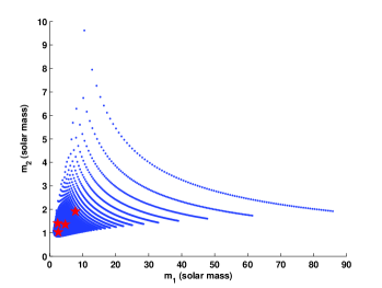
Figure 2: The region in the $m_{1}$, $m_{2}$ plane corresponding to the physically valid part of the $\tau_{0}$, $\tau_{1.5}$ plane. The region is indicated by taking a regular grid of points in the $\tau_{0}$, $\tau_{1.5}$ plane and mapping them to the corresponding values of $m_{1}$, $m_{2}$, where by convention $m_{1}\geq m_{2}$. The $\star$ markers shows the signal locations used in the simulations.

For each combination of signal location and SNR, 50 independent data realizations are generated. The length of each realization is $64$ sec, with $\delta_{s}=1/2048$ sec, and the signal is added at an offset of $10$ sec from the start.

V.1 Qualitative changes induced by a signal

It is instructive to observe how a signal affects the behavior of the swarm. In general, the presence of the signal leads to a broadening of the peak in the fitness function. As is well known, the broadening is more pronounced in one direction, due to the correlation between estimation errors, leading to the appearance of a thin ridge-like feature (c.f., Fig 1).

The particles begin by moving randomly in the parameter space but each time a particle crosses the ridge, its pbest tends to fall closer to the flanks of the ridge. As time progresses, the pbest of all particles cluster around the ridge. This increases its attractive power in the acceleration of the particles, progressively drawing more particles into exploration of the fitness function along the ridge.

Fig. 3 shows snapshots of PSO at different stages in the search and the progressive clustering of pbest locations is seen clearly. A key point to note here is that no prior knowledge is built into PSO about the ridge-like feature. It is found by the particles as they explore the search region.

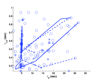
Figure 3: Evolution of a swarm in the presence of a signal. The ‘$\circ$’ and ‘$\ast$’ markers show the pbest locations of $N_{p}=81$ particles when 5% and 60% of the total number of steps were completed respectively. The lines show the paths followed by the pbest locations of 5 representative particles between these two steps. With time, the pbest locations tend to congregate around the ridge-like feature produced by a signal.

V.2 Figures of merit

In order to quantify the performance of PSO in the presence of a signal, we look at two figures of merit. The first is the probability of clustering defined in Sec. IV.1. Since the tuning procedure requires a minimum value of 90%, the probability of clustering in the presence of a strong signal should be significantly higher but it should be consistent with the pure noise case for weak signals.

When a signal is added to the data, we do not need the consistency of clustering criterion of Sec. IV.1 in order to confirm the association of a cluster with the global maximum. Since we know the location of the signal and since the expectation of the fitness function must be maximum at that location, it suffices to check if the maximum fitness in the cluster is larger than the value at the signal location. Our second figure of merit, therefore, is the fraction of trials in which this occurs. Ideally, this figure of merit should be unity.

Table 4 reports the first figure of merit for each combination of signal SNR and location. As expected, for the case of strong signals (SNR$\geq 7$) the probability of clustering is always, and often significantly, higher than 90%. For the weak signal SNR of $6.0$, the probability of clustering has an average value of 91% which is statistically consistent with the pure noise case of 90%.

Table 4: Probability of clustering for simulations with signal present in the data. For each combination of signal SNR and location, the fraction of trials (in %) $P_{\lambda}$, $P_{\tau_{0}}$ and $P_{\tau_{1.5}}$ for which the fitness, $\tau_{0}$ and $\tau_{1.5}$ values respectively were found to be clustered are listed. The probability of clustering, shown in bold, is the maximum over $P_{\lambda}$, $P_{\tau_{0}}$ and $P_{\tau_{1.5}}$. The number of trials for each combination is 50.

	$\begin{array}[]{c}(\tau_{0},\tau_{1.5})\\ =(5.0,0.6)\end{array}$	$(10.0,0.75)$	$(16.0,0.762)$	$(20.0,0.9)$
SNR=9.0	$\begin{array}[]{c}(P_{\lambda}){\bf 98}\\ (P_{\tau_{0}})94\\ (P_{\tau_{1.5}})94\end{array}$	$\begin{array}[]{c}{\bf 94}\\ 92\\ 94\end{array}$	$\begin{array}[]{c}94\\ {\bf 96}\\ 94\end{array}$	$\begin{array}[]{c}90\\ {\bf 98}\\ 94\end{array}$
8.0	$\begin{array}[]{c}96\\ {\bf 96}\\ 92\end{array}$	$\begin{array}[]{c}{\bf 98}\\ 96\\ 96\end{array}$	$\begin{array}[]{c}{\bf 98}\\ 92\\ 92\end{array}$	$\begin{array}[]{c}94\\ 92\\ {\bf 96}\end{array}$
7.0	$\begin{array}[]{c}{\bf 96}\\ 96\\ 90\end{array}$	$\begin{array}[]{c}{\bf 92}\\ 90\\ 88\end{array}$	$\begin{array}[]{c}{\bf 98}\\ 94\\ 98\end{array}$	$\begin{array}[]{c}{\bf 92}\\ 88\\ 90\end{array}$
6.0	$\begin{array}[]{c}92\\ {\bf 94}\\ 84\end{array}$	$\begin{array}[]{c}82\\ {\bf 86}\\ 86\end{array}$	$\begin{array}[]{c}{\bf 88}\\ 86\\ 84\end{array}$	$\begin{array}[]{c}94\\ {\bf 96}\\ 96\end{array}$

As far as the second figure of merit is concerned, we find that it is unity for all combinations of signal SNR and locations except for one, namely, $SNR=8.0$, $\tau_{0}=10.0$ sec and $\tau_{1.5}=0.75$ sec, for which it was 0.98. Fig. 4 shows the scatterplot between the maximum fitness found by PSO and the value at this signal location for all signal SNR values. It is seen that in one trial the maximum fitness fell below the value at the signal location. However, the two values are so close that the figure of merit should be considered to be practically unity for this case too.

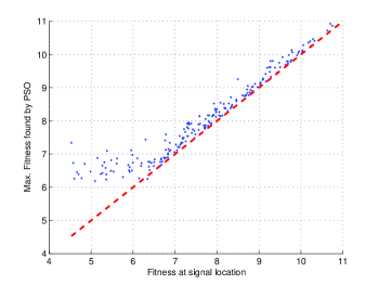
Figure 4: Scatterplot of maximum fitness value found by PSO (Y axis) against the value at the known signal location, $\tau_{0}=10.0$ sec, $\tau_{1.5}=0.75$ sec, for all signal SNR values. In one trial, the maximum fitness value (near 6.0 on the Y axis) dips below the line of equality (dashed).

Taken together, the figures of merit show that PSO almost always terminates near the true global maximum when a sufficiently strong signal is present. When the signal is weak, we recover the performance ensured by the tuning procedure for the pure noise case.

V.3 Signal detection and parameter estimation

In order to cast the results obtained so far in terms of signal detection and parameter estimation performance, we choose the maximum fitness value found over the $N_{rep}$ runs as the detection statistic and the location corresponding to the maximum fitness value as the estimator for the chirp time parameters.

V.3.1 Detection

It was discussed in Sec IV.3 that, after tuning PSO, the distribution of the detection statistic in trials with and without clustering remains the same. As the simultaneous clustering of the two chirp-times and the fitness values indicates termination in the vicinity of the global maximum, it follows that the probability distribution of the PSO detection statistic is about the same as that of the global maximum. Strictly speaking, the PSO detection statistic will always have a value less than the global maximum but, given our termination criterion, the relative difference between the two is less than 3%. Thus, the false alarm probabilities, for a given detection threshold, corresponding to the PSO detection statistic and the true global maximum are also nearly the same, with the former being slightly smaller.

In the presence of signals with an SNR of 8 or higher, which is the typical value sought in a real detection, it was shown that almost all trials exhibit clustering and that the detection statistic value was always higher than the fitness at the true signal location. Hence, the distribution of the detection statistic in the presence of a signal also closely follows that of the true global maximum. Strictly speaking, as with the false alarm probability, the detection probability will be slightly smaller for the PSO detection statistic, for a given threshold, as compared to that for the true global maximum.

The above line of reasoning suggests that the Receiver Operating Characteristics (ROC) of the PSO detection statistic should nearly be the same as that of the true global maximum. The only way to rigorously verify this is to carry out simulations with a large number of trials in which both PSO and grid-based searches are performed. This is a computationally expensive task which we plan to undertake in the future. However, it is important to note that such a comparison may not be possible for searches that are too expensive for a grid-based search.

V.3.2 Estimation

Table 5 summarizes the errors in the estimation of the chirp time parameters for signal SNR values $\geq 8$ at the different signal locations used in the simulations. Each entry in the table is an estimate of the root mean-square error (rmse) defined as,

$${\rm rmse}(\theta)=\left[E\left[\left(\widehat{\theta}-\theta\right)^{2}\right]\right]^{1/2}\;,$$ (20)

where $\widehat{\theta}$ is the estimator of $\theta$. The rmse includes the effects of both estimator variance and bias.

Since the search region in the current testbed includes unphysical chirp time parameters, the global maximum and, hence, the estimated chirp times fall there in some trials. Fig. 5 shows an example where the estimates from all the trials are shown for a signal SNR of 8. In an improved implementation of PSO, blocking the unphysical region should improve parameter estimation accuracy significantly. As an indicator of this, we also show in Table 5, the rmse obtained by dropping the trials where the estimate fell in the unphysical region. It is seen that the errors are reduced significantly, especially for the lower signal SNR value for which there is more scatter into the the unphysical region.

A comparison of Table 5 with existing results balasubramanian96 shows that the estimation errors due to PSO are consistent with grid-based searches.

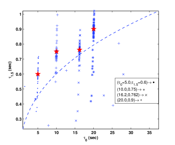
Figure 5: Estimation of parameter values for a signal SNR of 8.0. The true locations of the signals are indicated by the $\star$ marker and each of the markers, $\bullet$, $+$, $\ast$ and $\times$, indicates an estimated location corresponding to one of the true locations. The association between the markers and the true signal locations is indicated in the figure. For each true signal location, the simulation consisted of 50 trials.

Table 5: Signal parameter estimation errors with PSO. Each entry in the table is of the form $a(b)$, where $a$ and $b$ are the estimated root mean square errors (rmse) for $\tau_{0}$ and $\tau_{1.5}$ respectively (expressed as a percentage of the true parameter value). In each row, the top and bottom pairs of numbers refer to mse obtained without and with the physical boundary cut respectively. All the numbers have been rounded off, given the expected precision from the 50 trials used per combination of signal SNR and location.

	$\begin{array}[]{c}(\tau_{0},\tau_{1.5})\\ =(5.0,0.6)\end{array}$	$(10.0,0.75)$	$(16.2,0.762)$	$(20.0,0.9)$
SNR=9.0	$\begin{array}[]{c}2(13)\\ 2(12)\end{array}$	$\begin{array}[]{c}1(11)\\ 0.5(6)\end{array}$	$\begin{array}[]{c}0.3(6.0)\\ 0.2(4)\end{array}$	$\begin{array}[]{c}1(11)\\ 0.2(4)\end{array}$
8.0	$\begin{array}[]{c}44(13)\\ 10.5(10)\end{array}$	$\begin{array}[]{c}32(16)\\ 1(10)\end{array}$	$\begin{array}[]{c}12(16)\\ 0.3(5)\end{array}$	$\begin{array}[]{c}11(17)\\ 12(10)\end{array}$

V.4 Computational cost

The number of fitness function evaluations for each combination of signal SNR and location are shown in Table. 6. It is seen that for a signal SNR of 9.0, the maximum number of evaluations is about the same as the mean in the pure noise case (c.f., Table 1). This reduction is consistent with the fact that a strong signal makes it easier for the swarm to find the global maximum.

Table 6: Computational cost of PSO on data containing a signal. For each combination of signal SNR and location, the mean number of fitness function evaluations, over $50$ trials, is listed along with the maximum (superscript) and minimum (subscript). All numbers are in units of $10^{4}$ and rounded off to a single digit of precision.

	$\begin{array}[]{c}(\tau_{0},\tau_{1.5})\\ =(5.0,0.6)\end{array}$	$(10.0,0.75)$	$(16.0,0.762)$	$(20.0,0.9)$
SNR=9.0	$4.4_{3.8}^{5.2}$	$4.7_{4.1}^{5.7}$	$4.8_{4.2}^{5.6}$	$4.7_{4.2}^{5.8}$
8.0	$4.5_{3.8}^{6.0}$	$4.7_{3.7}^{6.5}$	$4.8_{4.1}^{5.6}$	$4.8_{4.2}^{5.9}$
7.0	$4.7_{3.6}^{6.4}$	$4.8_{3.9}^{6.3}$	$4.9_{3.7}^{6.2}$	$4.8_{3.8}^{5.9}$
6.0	$4.5_{3.3}^{6.1}$	$4.8_{2.9}^{7.0}$	$4.7_{3.2}^{5.9}$	$4.7_{3.6}^{6.0}$

For ground-based detectors, the dominant computational cost comes from the pure noise case. Although our tuning procedure produced $N_{p}=81$ and $N_{t}=80$ as the optimal combination, there is statistical uncertainty in this result due to the finite and somewhat small number of trials used. To make our estimate of the computational cost conservative, we use the combination $N_{p}=121$ and $N_{t}=80$ instead for which all the performance measures are significantly better. From Table 1, the typical number of fitness evaluations required for the testbed considered here is $\sim 7\times 10^{4}$ with a spread of about $\pm 2\times 10^{4}$. Of this, the termination criterion itself accounts for a fixed number, $(N_{t}=80)\times(N_{p}=121)=9680$, of evaluations.

A grid-based search provides a convenient perspective for evaluating the computational cost of PSO. According to (owen99, ), for 2PN waveform and initial LIGO noise PSD, the number of fitness function evaluations required in a single grid with a minimal match of 0.97 ($\Rightarrow\alpha=0.03$) is $1.1\times 10^{4}$ if the minimum mass used for constructing the template waveforms is $1M_{\odot}$. In the current testbed, the search region in the mass plane (c.f., Fig. 2) is not the simple one considered in owen99 although the minimum masses are similar. Additionally, (owen99, ) uses an analytic fit for the noise PSD that differs from the one used here. Ignoring these differences we find that the current implementation of PSO requires about 7 times as many evaluations, on the average, as a grid-based method.

VI Conclusions

We applied PSO to the binary inspiral testbed where the main challenge was to locate the global maximum of a highly multi-modal fitness function. Such functions, with an unpredictable number of extrema having random locations and sizes, are typical in GW data analysis.

In response to the questions posed at the beginning, the results obtained from simulations show clearly that:

1. PSO is a viable method for signal detection and estimation in GW data analysis as it can successfully handle the challenge of high multi-modality presented by such problems.

2. Good performance was achieved by tuning only two out of the nine design variables involved in the method. Thus, PSO is a stochastic method that offers the possibility of having a small number of design variables in practice.

3. The design variables were tuned using a systematic procedure that does not require any prior information about features of the fitness function. As such, the procedure should be widely applicable to other stochastic methods also.

4. PSO is about 7 times more expensive than a grid-based search in the number of fitness function evaluations required.

The higher cost of PSO is not surprising since grid-based searches are usually more efficient than stochastic methods in low-dimensional problems such as the one considered here. The performance gain of stochastic methods appears due to the slower rise in their computational cost, with increase in dimensionality, compared to the exponential one of grid-based searches. Therefore, we expect PSO to be cheaper than grid-based searches in higher dimensional problems. However, a definitive answer requires an actual test on problems such as the inspiral of high mass spinning binary components or the LISA Galactic Binary resolution problem babak+etal:mldc2 . The demonstration in this paper that PSO can handle the more serious challenge of high multi-modality is the first step towards such future investigations.

The computational cost of PSO may be significantly reduced by taking into account the physical boundary in parameter space (see Fig. 5). The current implementation of PSO requires the search to extend over a large unphysical region. In fact, as far as the binary inspiral problem goes, we find this to be the most outstanding issue. We have tried the invisible walls condition with the curved physical boundary but find that the performance of PSO is negatively affected. Specifically, termination takes a much longer time and the probability of clustering is significantly reduced. This behavior is attributable to the curved shape of the boundary allowing a significantly larger number of particles to escape the search domain. Once outside, particles contribute nothing to the search and keep moving until they are pulled back.

To solve this problem, it appears inevitable that the dynamical equations of PSO must be modified. For signals other than binary inspirals, such as Galactic Binaries in the case of LISA, the nature of the boundary problem would be different and it may not be an issue in some applications.

Finally, a comment about the use of Gaussian, stationary noise in the testbed. We emphasize here that PSO is a method for finding the global maximum of a fitness function irrespective of what produces that peak, a genuine GW signal or an instrumental transient. Since, the implementation of PSO in this paper uses no prior information about features of the fitness function, it should find the peak regardless of its source. Thus, there should be no significant difference in the performance of PSO and a grid-based method even for non-stationary, non-Gaussian noise. In future work, we will verify this explicitly by using non-GW signals in our simulations.

Appendix A Details of the signal waveform

A.1 Chirp-time parameters

The chirp-time parameters, $\{\tau_{a}\}$, $a=0,1,1.5,2$, are given in terms of the masses, $m_{1}$ and $m_{2}\leq m_{1}$, of the binary components (we use $c=G=1$),

$$\tau_{0} = \frac{5}{256}M^{-5/3}\eta^{-1}(\pi f_{a})^{-8/3}\;,$$ (21)

$$\tau_{1} = \frac{5}{192\mu(\pi f_{a})^{2}}\left(\frac{743}{336}+\frac{11}{4}\eta\right)\;,$$ (22)

$$\tau_{1.5} = \frac{1}{8\mu}\left(\frac{M}{\pi^{2}{f_{a}}^{5}}\right)^{1/3}\;,$$ (23)

$$\tau_{2} = \frac{5}{128\mu}\left(\frac{M}{\pi^{2}{f_{a}}^{2}}\right)^{2/3}\left(\frac{3058673}{1016064}+\frac{5429}{1008}\eta+\right.$$ (24)

$$\left.\frac{617}{144}\eta^{2}\right)\;,$$

where $M=m_{1}+m_{2}$ is the total mass of the compact binary, $\mu=m_{1}m_{2}/M$ is the reduced mass and $\eta=\mu/M$.

Since all the chirp time parameters depend on $m_{1}$ and $m_{2}$, only two of them are independent. It is convenient to choose $\tau_{0}$ and $\tau_{1.5}$ as the independent parameters since $M$ and $\mu$ can be obtained algebraically from them,

$$\mu = \frac{1}{16f_{a}^{2}}\left(\frac{5}{4\pi^{4}\tau_{0}\tau_{1.5}^{2}}\right)^{1/3}\;,$$ (25)

$$M = \frac{5}{32f_{a}}\frac{\tau_{1.5}}{\pi^{2}\tau_{0}}\;,$$ (26)

allowing $\tau_{1}$ and $\tau_{2}$ to be obtained algebraically from $\tau_{0}$ and $\tau_{1.5}$.

A.2 The phase function

In Eq. 6, the function $\psi(f;\theta)$ is given by,

$$\psi(f;\theta) = \sum_{i\in\{0,1,1.5,2\}}\!\!\!\alpha_{i}(f)\tau_{i}\;,$$ (27)

$$\alpha_{0}(f) = 2\pi f-\frac{16\pi f_{a}}{5}+\frac{6\pi f_{a}}{5}\left(\frac{f}{f_{a}}\right)^{-5/3}\;,$$ (28)

$$\alpha_{1}(f) = 2\pi f-4\pi f_{a}+2\pi f_{a}\left(\frac{f}{f_{a}}\right)^{-1}\;,$$ (29)

$$\alpha_{1.5}(f) = -2\pi f+5\pi f_{a}-3\pi f_{a}\left(\frac{f}{f_{a}}\right)^{-2/3}\;,$$ (30)

$$\alpha_{2}(f) = 2\pi f-8\pi f_{a}+6\pi f_{a}\left(\frac{f}{f_{a}}\right)^{-1/3}\;.$$ (31)

The functions $\alpha_{a}$, $a=0,1,1.5,2$ and the $f^{-7/6}$ factor in the amplitude of the signal (Eq. 6) can be pre-computed and stored, reducing the computational cost of generating waveforms.