Bridging length and time scales in sheared demixing systems: from the Cahn-Hilliard to the Doi-Ohta model

Abstract

We develop a systematic coarse-graining procedure which establishes the connection between models of mixtures of immiscible fluids at different length and time scales. We start from the Cahn-Hilliard model of spinodal decomposition in a binary fluid mixture under flow from which we derive the coarse-grained description. The crucial step in this procedure is to identify the relevant coarse-grained variables and find the appropriate mapping which expresses them in terms of the more microscopic variables. In order to capture the physics of the Doi-Ohta level, we introduce the interfacial width as an additional variable at that level. In this way, we account for the stretching of the interface under flow and derive analytically the convective behavior of the relevant coarse-grained variables, which in the long wavelength limit recovers the familiar phenomenological Doi-Ohta model. In addition, we obtain the expression for the interfacial tension in terms of the Cahn-Hilliard parameters as a direct result of the developed coarse-graining procedure. Finally, by analyzing the numerical results obtained from the simulations on the Cahn-Hilliard level, we discuss that dissipative processes at the Doi-Ohta level are of the same origin as in the Cahn-Hilliard model. The way to estimate the interface relaxation times of the Doi-Ohta model from the underlying morphology dynamics simulated at the Cahn-Hilliard level is established.

I Introduction

The problem of coarse graining in terms of bridging time and length scales between microscopic and macroscopic levels of description is a crucial issue in the physics of complex fluids, like polymer melts, colloids, liquid crystals and emulsions, out of equilibrium. The wide span of length and time scales is particularly evident in these systems, due to their internal structure leading to additional mesoscopic levels of description, intermediate between microscopic and macroscopic Larson_99 . Many of the practical applications of these fluids crucially depend on the evolution of their complex, multiphase morphologies developed through equilibrium self-assembling or during non-equilibrium processing of these systems. Some examples of such applications are food processing, membrane technology, encapsulation systems, drug delivery, coating, production of paint and cosmetics etc Larson_99 ; complex_fluids-1 ; complex_fluids-2 ; complex_fluids-3 . Therefore, the goal of connecting different levels of description of complex fluids is of great importance. In the present work, this problem is approached by considering the phase separation of binary fluid mixtures subjected to a shear flow.

When a binary (AB) fluid mixture is quenched from a high temperature homogeneous phase to an unstable region below the coexistence curve, it becomes unstable with respect to long-wavelength fluctuations in the composition and starts to phase separate Bray-94 . The interface between the A- and B-rich domains is initially very diffuse, but sharpens with time. In the later stages of phase separation, local equilibrium is achieved within each domain and the effects of interfacial energy become important. The domain pattern further coarsens in time, while the dynamics is governed by the minimization of the excess interfacial energy of the system. The kinetics of this nonequilibrium phenomena is an area of extensive research Bray-94 . Especially the effects of a shear flow on the deformation and kinetics of domain growth, and the corresponding rheological behavior, are challenging and technologically important topics Onuki-97R . The complexity of the problem lies in the presence of a complex interface and its motions due to coagulation, rupture and deformation of domains, which significantly influences the macroscopic properties of a mixture. Although numerous experimental KrSengHam_92 ; Lauger-95 ; Matsuzaka-98 ; Derks-08 ; Aarts-05 , numerical OhtaNozDoi_90 ; PadTox_97 ; CorGonLam-1 ; CorGonLam-2 ; CorGonLam-3 ; CorGonLam-4 ; Zhang_00 ; Berth_01 ; Fielding_08 ; ShouChakr_00 ; NESS-1 ; NESS-2 ; NESS-3 and analytical Onuki_87 ; DoiOhta_91 ; CorGonLam-1 ; CorGonLam-2 ; CorGonLam-3 ; CorGonLam-4 ; Fielding_08 ; CH-analytical-1 ; CH-analytical-2 studies have been done in order to understand the flow effects on the morphology and the dynamics in this system, many questions still remain open, like the possibility of achieving a nonequilibrium steady state ShouChakr_00 ; NESS-1 ; NESS-2 ; NESS-3 ; Fielding_08 .

Due to the complex morphology of this system, even in the case of two simple Newtonian fluids, one can identify several length and time scales requiring different theoretical approaches and simulation methods. The standard mesoscopic model for understanding the dynamics of spinodal decomposition is based on the formulation of Cahn and Hilliard CaHil_58 . It describes the kinetics of the system in terms of the convective-diffusion equation for the order parameter - composition $c$, and the Navier-Stokes equation for the fluid velocity $\mathbf{v}$ (so-called ‘model H’, see e.g. model-H ):

$$\frac{\partial c}{\partial t}+\mathbf{v}\cdot\left(\nabla c\right) = M\nabla^{2}\mu_{c},$$ (1a)

$$\rho\left(\frac{\partial\mathbf{v}}{\partial t}+\left(\mathbf{v}\cdot\nabla\right)\mathbf{v}\right) = \eta\nabla^{2}\mathbf{v}-\nabla p+\mu_{c}\nabla c,$$ (1b)

where $M$ is the mobility coefficient, $p$ the pressure, $\rho$ the mass density, and $\eta$ the viscosity. The chemical potential $\mu_{c}$ is given as $\mu_{c}=\delta F\left[c\right]/\delta c$, with the free energy functional of the Ginzburg-Landau form $F\left[c\right]=\int d^{3}r\left(-(a/2)c^{2}+(b/4)c^{4}+(\kappa/2)\left|\nabla c\right|^{2}\right)$, $(a,b>0)$, where the square brackets emphasize the occurence of functional integrations. During the late stages of phase separation, the time evolution can be described by the change of the size and shapes of the domains. Due to the dynamical scaling hypothesis, the system is described by a characteristic length scale $L(t)$, which is related to the average domain size. By using dimensional arguments, one can estimate the size of the contributions from the specific terms in the equations (1), which leads to the distinction of the three growth regimes Bray-94 ; Sigg_79 ; Furuk_85 : diffusive $L(t)\sim\left(M\sigma t\right)^{1/3}$, viscous hydrodynamics $L(t)\sim\sigma t/\eta$, and inertial hydrodynamics $L(t)\sim\left(\sigma t^{2}/\rho\right)^{1/3}$, where $\sigma$ is the interfacial tension. Under shear flow the situation becomes more complex since the domains elongate along the flow direction and the system becomes anisotropic and can not be described by a single length scale (see ShouChakr_00 ; CorGonLam-1 ; CorGonLam-2 ; CorGonLam-3 ; CorGonLam-4 ; Berth_01 and references therein).

On the other hand, for understanding the rheological properties of multiphase systems, like polymer blends, under shear flow, Doi and Ohta suggested that the average information about the interface between the two phases is sufficient. Hence, their phenomenological model DoiOhta_91 focus on the interface, which is considered as a zero width surface embedded in the fluid. The presence of the interface is then represented through two state variables that describe the interfacial area per unit volume, $Q$, and its anisotropy, $\mathbf{q}$, in a given flow field. They are defined in terms of the interface orientational distribution function $f\left(\mathbf{n}\right)$, where $\mathbf{n}$ is a unit vector normal to the interface. This is a probability density of finding the amount of interface with the orientation $\mathbf{n}$, so that the integral over all orientations gives the total amount of interface per unit volume. Therefore, for the state variables $Q$ and $\mathbf{q}$ one can write the following definitions

$$Q = \int f\left(\mathbf{n}\right)d^{2}n,$$ (2a)

$$\mathbf{q} = \int\left(\mathbf{nn}-\frac{1}{3}\mathbf{1}\right)f\left(\mathbf{n}\right)d^{2}n=\overline{\mathbf{nn}}-\frac{1}{3}Q\mathbf{1},$$ (2b)

where $\mathbf{1}$ is the unit tensor, and $\int d^{2}n$ denotes an integration over the unit sphere. Introduction of the distribution function and further averaging over all possible orientations imply the loss of information of the detailed morphology of the system. This coarse-grained model keeps only the information about the average amount of interfacial area per unit volume and its orientation. However, the detailed information about the morphology, i.e., the explicit interfacial position and orientation, is lost.

The time evolution of the new configurational variables $Q$ and $\mathbf{q}$ is determined by two factors: the external flow field which orients and enlarges the interface, and the interfacial tension which has the opposite effect and governs the relaxation of the interface. Therefore, the time evolution can be separated into two parts:

$$\frac{\partial Q}{\partial t} = \left.\frac{\partial Q}{\partial t}\right|_{\rm convection}+\left.\frac{\partial Q}{\partial t}\right|_{\rm relaxation},$$ (3a)

$$\frac{\partial\mathbf{q}}{\partial t} = \left.\frac{\partial\mathbf{q}}{\partial t}\right|_{\rm convection}+\left.\frac{\partial\mathbf{q}}{\partial t}\right|_{\rm relaxation}.$$ (3b)

The convective part of the time evolution can be found by considering the convection behavior of the unit vector $\mathbf{n}$ normal to the interface under affine deformations and volume preservation assumptions. Then, the convection of the state variables is derived using the above definitions (2)

$$\left.\frac{\partial Q}{\partial t}\right|_{\rm convection} = -\nabla\cdot\left(Q\mathbf{v}\right)-\left(\nabla\mathbf{v}\right)^{\rm T}:\mathbf{q}+\frac{2}{3}Q\mathbf{1}:\left(\nabla\mathbf{v}\right)^{\rm T},$$ (4a)

$$\left.\frac{\partial\mathbf{q}}{\partial t}\right|_{\rm convection} = -\left(\nabla\mathbf{v}\right)\cdot\mathbf{q}-\mathbf{q}\cdot\left(\nabla\mathbf{v}\right)^{\rm T}-\frac{1}{3}Q\dot{\bm{\gamma}}-\mathbf{v}\cdot\nabla\mathbf{q}+\frac{1}{3}\mathbf{1}\left(\nabla\mathbf{v}\right):\mathbf{q}$$ (4b)

$$+\left[\mathbf{q}+\frac{1}{9}Q\mathbf{1}\right]{\rm Tr}\left(\nabla\mathbf{v}\right)+\overline{\mathbf{nnnn}}:\left(\nabla\mathbf{v}\right)^{\rm T}.$$

where $\dot{\bm{\gamma}}=\nabla\mathbf{v}+\left(\nabla\mathbf{v}\right)^{T}$ is the symmetrized velocity gradient tensor WagOttEdw_99 . In the equation for the interfacial shape (4b), the fourth moment of the interface normal $\mathbf{n}$ appears, which must be expressed in terms of the state variables through an appropriate closure approximation in order to obtain a self-contained set of time evolution equations. Doi and Ohta postulated the following closure approximation

$$\overline{\mathbf{nnnn}}:\left(\nabla\mathbf{v}\right)^{\rm T}=\frac{1}{Q}\overline{\mathbf{nn}}\;\overline{\mathbf{nn}}:\left(\nabla\mathbf{v}\right)^{\rm T}$$ (5)

and verified its accuracy. Using definition (2b), the convective time evolution of the anisotropy $\mathbf{q}$ takes the form

$$\left.\frac{\partial\mathbf{q}}{\partial t}\right|_{\rm convection} = -\left(\nabla\mathbf{v}\right)\cdot\mathbf{q}-\mathbf{q}\cdot\left(\nabla\mathbf{v}\right)^{\rm T}-\frac{1}{3}Q\dot{\bm{\gamma}}-\mathbf{v}\cdot\nabla\mathbf{q}+\frac{1}{3}\mathbf{1}\left(\nabla\mathbf{v}\right):\mathbf{q}$$ (6)

$$+\left[\mathbf{q}+\frac{1}{9}Q\mathbf{1}\right]{\rm Tr}\left(\nabla\mathbf{v}\right)+\frac{1}{Q}\left(\mathbf{q}+\frac{1}{3}Q\mathbf{1}\right)\left(\mathbf{q}+\frac{1}{3}Q\mathbf{1}\right):\left(\nabla\mathbf{v}\right).$$

As for the relaxation in the Doi-Ohta model, the relaxation of the state variables can be written in a generalized form

$$\left.\frac{\partial Q}{\partial t}\right|_{\rm relaxation} = -\,\frac{1}{\tau_{\rm do,1}}Q,$$ (7a)

$$\left.\frac{\partial\mathbf{q}}{\partial t}\right|_{\rm relaxation} = -\,\frac{1}{\tau_{\rm do,2}}\mathbf{q}.$$ (7b)

In order to specify the empirical interface relaxation times $\tau_{\rm do,1}$ and $\tau_{\rm do,2}$, assumptions on the appropriate interface relaxation mechanisms must be made. Finally, the full set of time evolution equations for the configurational variables $Q$ and $\mathbf{q}$, together with the equations for the hydrodynamic variables $\rho$, $\mathbf{g}$ and $\epsilon$ has been formulated within the GENERIC formalism WagOttEdw_99 , which for the stress tensor gives

$$\bm{\Sigma}=-\bm{\tau}-\sigma\left(\mathbf{q}-\frac{2}{3}Q\mathbf{1}\right)-p\mathbf{1},$$ (8)

where $\bm{\tau}$ is the viscous stress tensor.

Although very crude, the ability of the Doi-Ohta model to connect the morphology of the system to its macroscopic behavior, through the above given set of rheological constitutive equations, is very appealing for different theoretical and technological purposes. The model and its variants have been used to analyze multiphase flow of polymers, as well as simple fluids undergoing spinodal decomposition LeePark_94 ; DO-different-1 ; DO-different-2 ; DO-different-3 ; DO-different-4 ; DO-different-5 ; DO-different-6 ; WagOttEdw_99 ; KrSengHam_92 . However, the need for explicit assumptions of the interfacial relaxation mechanisms and the appropriate relaxation times, which depend in an unknown manner on the underlying morphology, makes it difficult for wide and easy use. Therefore, in this paper we concentrate on relating the macroscopic Doi-Ohta model to the underlying morphology, described by the more detailed Cahn-Hilliard model. The goal is to establish a systematic, thermodynamically guided method which determines the coarse-grained Doi-Ohta model of a phase separating binary fluid from the more detailed Cahn-Hilliard model, in the region where the considered system can be described with both approaches. To connect these two different levels of description, the General Equation for the Non-Equilibrium Reversible-Irreversible Coupling (GENERIC) framework is used hco ; OttGrm-97a ; OttGrm-97b . This approach allows to specify the mathematical structure which should be left invariant in the coarse-graining procedure and hence assures thermodynamically consistent results.

In the following, we first describe the GENERIC structure and formulate the Cahn-Hilliard model within this framework. The coarse-graining procedure which derives the more macroscopic Doi-Ohta model is then presented. In particular, we present some mathematical challenges which occur within the coarse-graining procedure, as well as the efficient way to extract the interface relaxation times of the Doi-Ohta level from the underlying morphology.

II GENERIC formalism

The main points of the GENERIC framework of nonequilibrium thermodynamics hco ; OttGrm-97a ; OttGrm-97b can be summarized in the following way. In analogy to equilibrium thermodynamics, one needs to choose a complete set of variables $\mathbf{x}$, which describes the situation of interest to the desired detail. For a system out of equilibrium the time evolution of all the relevant state variables can be divided into the reversible and the irreversible contributions

$$\dot{\mathbf{x}}=\dot{\mathbf{x}}|_{\rm rev}+\dot{\mathbf{x}}|_{\rm irrev}\;.$$ (9)

These two contributions are obtained by considering separately the energy $E$ and the entropy $S$ — the two generators of reversible and irreversible dynamics, respectively. This can be explained by using the analogy with the classical Hamiltonian mechanics as following. Using the classical Hamiltonian mechanics, the reversible contribution of the time evolution, $\dot{\mathbf{x}}|_{\rm rev}$, is related to the energy gradient by way of a Poisson operator ${\mathbf{L}}$, so that it is $\dot{\mathbf{x}}|_{\rm rev}={\mathbf{L}}\cdot(\delta E/\delta{\mathbf{x}})$. The Poisson bracket associated to ${\mathbf{L}}$, given by $\{A,B\}=(\delta A/\delta{\mathbf{x}},{\mathbf{L}}\cdot\delta B/\delta{\mathbf{x}})$ with appropriate scalar product $(.,.)$, must be antisymmetric and satisfy Lebniz’ rule and the Jacobi identity, which are both features that capture the nature of reversibility. The motivation for formulating the irreversible part of the dynamics comes from the reversible part. For the reversible dynamics, the energy plays a distinct role — it is a conserved quantity for closed systems and it drives the reversible dynamics. Therefore, for the irreversible dynamics the entropy presents an important quantity — it does not decrease for closed systems. For the GENERIC formulation, it is then assumed that the irreversible contribution to the time evolution, $\dot{\mathbf{x}}|_{\rm irrev}$, is driven by the entropy gradient, i.e., that it is of the form $\dot{\mathbf{x}}|_{\rm irrev}={\mathbf{M}}\cdot(\delta S/\delta{\mathbf{x}})$, with ${\mathbf{M}}$ a generalized friction matrix. This friction matrix contains transport coefficients and relaxation times associated to the corresponding dissipative effects. It is required for ${\mathbf{M}}$ to be (Onsager-Casimir) symmetric and the condition that it is positive semi-definite ensures that $\dot{S}\geq 0$ is fulfilled.

From the above illustration, one concludes that the time evolution of $\mathbf{x}$ can be expressed in terms of four “building blocks” $E$, $S$, $\mathbf{L}$ and $\mathbf{M}$ as

$$\dot{\mathbf{x}}={\mathbf{L}}(\mathbf{x})\cdot\frac{\delta E(\mathbf{x})}{\delta\mathbf{x}}+{\mathbf{M}}(\mathbf{x})\cdot\frac{\delta S(\mathbf{x})}{\delta\mathbf{x}}\;.$$ (10)

The two different contributions to the time evolution, reversible and irreversible, are not independent. They are related by the two complementary degeneracy requirements

$${\mathbf{L}}(\mathbf{x})\cdot\frac{\delta S(\mathbf{x})}{\delta\mathbf{x}}=\mathbf{0}\;,\;\;\;{\mathbf{M}}(\mathbf{x})\cdot\frac{\delta E(\mathbf{x})}{\delta\mathbf{x}}=\mathbf{0}\;.$$ (11)

The first requirement expresses the reversible nature of the $\mathbf{L}$ contribution to the dynamics, demonstrating the fact that the reversible dynamics captured in $\mathbf{L}$ does not affect the entropy functional. The second one expresses the conservation of the total energy of an isolated system by the irreversible contribution to the system dynamics captured in $\mathbf{M}$.

The presented GENERIC form of the time evolution equations for the state variables $\mathbf{x}$ represents a mathematical structure which guarantees that the chosen model is thermodynamically consistent. Moreover, by concentrating on the thermodynamics building blocks $E$, $S$, $\mathbf{L}$ and $\mathbf{M}$ rather than on the time evolution equations in systematic coarse-graining procedures, the obtained coarse-grained equations are guaranteed to be also thermodynamically admissible.

II.1 GENERIC formulation of the Cahn-Hilliard model

In order to develop a systematic coarse-graining procedure which relates the more detailed Cahn-Hilliard level to the more macroscopic Doi-Ohta level, we must formulate the first one in the GENERIC structure. As a first step, we need to identify the list of independent variables $\mathbf{x}$ which fully describe the considered thermodynamic system. In addition to the hydrodynamic fields, the mass density $\rho$, the momentum density $\mathbf{g}$, and the internal energy density $\epsilon$, we use the composition $c$ – the mass fraction of one component – in order to describe the configuration of the system.

Taking into account the Cahn-Hilliard free energy of a phase separating binary system, we assume the total energy and entropy of the system, in terms of the variables ${\mathbf{x}}=\left(\rho,{\bf g},\epsilon,c\right)$, to be

$$E^{\rm(1)}({\mathbf{x}}) = \int_{V}d^{3}r\,\left(\frac{1}{2}\frac{{\mathbf{g}}^{2}}{\rho}+\epsilon+\frac{1}{2}\kappa_{\rm E}\left|\nabla c\right|^{2}\right),$$ (12a)

$$S^{\rm(1)}({\mathbf{x}}) = \int_{V}d^{3}r\,s\left(\rho,\epsilon,c\right),$$ (12b)

where $V$ is the total volume of the system. For simplicity, the gradient-squared term, which describes the contribution due to the presence of the interface, is included only in the energy functional (12a), although it can be separated between both, energy and entropy Onu_05 ; Jelic_09 . The actual functional form of the entropy density $s\left(\rho,\epsilon,c\right)$ is not needed for the derivation of the Cahn-Hilliard time evolution equations in the GENERIC form. However, we use the assumption of local equilibrium, i.e., $s\left(\rho,\epsilon,c\right)$ has the same form as an equilibrium system at the corresponding state point. In the numerical simulations reported in this paper, we have used the popular $c^{4}$-structure for the uniform part of the entropy density, i.e., $s\left(\rho,\epsilon,c\right)=s_{0}\left(\rho,\epsilon\right)-ac^{2}/2+bc^{4}/4$, which presents the entropic contribution to the bulk free energy density CorGonLam-1 ; CorGonLam-2 ; Berth_01 ; ShouChakr_00 ; NESS-2 ; NESS-3 ; Fielding_08 . Other possible functional forms include the one for the van der Waals systems, for example Eq. $4$ in Onu_05 . The functional derivatives of the above energy and entropy functionals with respect to the independent variables $\mathbf{x}$ are given with

$$\frac{\delta E^{\rm(1)}}{\delta{\mathbf{x}}} = \left(-\frac{1}{2}{\mathbf{v}}^{2},{\mathbf{v}},1\,,-\kappa_{\rm E}\nabla^{2}c\right)^{\rm T},$$ (13a)

$$\frac{\delta S^{\rm(1)}}{\delta{\mathbf{x}}} = \left(\frac{\partial s\left(\rho,\epsilon,c\right)}{\partial\rho},{\mathbf{0}}\,,\frac{1}{T}\,,\frac{\partial s\left(\rho,\epsilon,c\right)}{\partial c}\right)^{\rm T},$$ (13b)

where we omitted the position dependence for simplicity.

The Poisson operator ${\mathbf{L}}^{\rm(1)}$ determines the reversible contributions to the full evolution equations of the variables ${\mathbf{x}}$, and hence models the convective behavior. For our particular choice of variables and in view of the functional derivatives (13) one arrives at the following expression for the Poisson operator

$${\mathbf{L}}^{\rm(1\,)}\left(\mathbf{r},\mathbf{r^{\prime}}\right)=\left(\begin{array}[]{cccc}0&\rho\left(\mathbf{r^{\prime}}\right)\frac{\partial\delta}{\partial\mathbf{r^{\prime}}}&0&0\\ -\frac{\partial\delta}{\partial\mathbf{r}}\,\rho\left(\mathbf{r}\right)&L^{\rm(1\,)}_{gg}&L^{\rm(1\,)}_{g\epsilon}&-\left(\nabla c\left(\mathbf{r}\right)\right)\delta\\ 0&L^{\rm(1\,)}_{\epsilon g}&0&0\\ 0&-\left(\nabla c\left(\mathbf{r}\right)\right)\delta&0&0\end{array}\right),$$ (14e)

with

$$L^{\rm(1\,)}_{gg}\left(\mathbf{r},\mathbf{r^{\prime}}\right) = {\mathbf{g}}\left(\mathbf{r^{\prime}}\right)\frac{\partial\delta}{\partial\mathbf{r^{\prime}}}-\frac{\partial\delta}{\partial\mathbf{r}}{\mathbf{g}}\left(\mathbf{r}\right),$$ (14f)

$$L^{\rm(1\,)}_{g\epsilon}\left(\mathbf{r},\mathbf{r^{\prime}}\right) = -\frac{\partial\delta}{\partial\mathbf{r}}\,\epsilon\left(\mathbf{r}\right)-\frac{\partial\delta}{\partial\mathbf{r}}p\left(\mathbf{r^{\prime}}\right),$$ (14g)

$$L^{\rm(1\,)}_{\epsilon g}\left(\mathbf{r},\mathbf{r^{\prime}}\right) = \epsilon\left(\mathbf{r^{\prime}}\right)\frac{\partial\delta}{\partial\mathbf{r^{\prime}}}+p\left(\mathbf{r}\right)\frac{\partial\delta}{\partial\mathbf{r^{\prime}}}\,,$$ (14h)

where $\delta=\delta\left(\mathbf{r}-\mathbf{r^{\prime}}\right)$ is Dirac’s $\delta$-function. In addition to the usual hydrodynamic part of the Poisson matrix for the variables $\rho$, $\mathbf{g}$, $\epsilon$, element $L^{\rm(1\,)}_{cg}$ dictates the convection of the configurational variable $c$, which is a scalar, so the entry in the Poisson operator is as expected by hco . The antisymmetry of the Poisson matrix (14) and the degeneracy requirement are satisfied by construction, and the Jacobi identity holds. At this point we mention that, in general, the symbol “$\cdot$” in (10) implies not only summation over discrete indices. If field variables are involved the operators $\mathbf{L}$ and $\mathbf{M}$ are written in terms of two space arguments $\left({\mathbf{r}},{\mathbf{r^{\prime}}}\right)$, and an integration over ${\mathbf{r^{\prime}}}$ must be performed when multiplied with a function of $\mathbf{r^{\prime}}$ from the right. However, in the case of the field equations being local, one can express $\mathbf{L}$ and $\mathbf{M}$ in terms of a single variable $\mathbf{r}$ only hco , and no integration is implied when these operators are multiplied from the right. Such single variable notation is used below for the friction matrix ${\mathbf{M}}^{\rm(1\,)}$.

The irreversible effects in the Cahn-Hilliard model for a binary fluid under flow arise due to viscosity and heat conduction, as well as diffusion. Thus, to incorporate them through the friction matrix ${\mathbf{M}}^{\rm(1\,)}$, one can write it as the sum of two matrices $\mathbf{M}^{\rm(1\,)}=\mathbf{M}^{\rm(1\,),hyd}+\mathbf{M}^{\rm(1\,),dif}$, where $\mathbf{M}^{\rm(1\,),hyd}$ is the usual hydrodynamic friction matrix, and $\mathbf{M}^{\rm(1\,),dif}$ contains all the transport coefficients related to diffusion of mass EspTh_03 ; hco . The hydrodynamic part of the friction matrix is given in the $\mathbf{r}$-notation as

$$\mathbf{M}^{\rm(1\,),hyd}\left(\mathbf{r}\right)=\left(\begin{array}[]{cccc}0&0&0&0\\ 0&M^{\rm(1\,),hyd}_{gg}&M^{\rm(1\,),hyd}_{g\epsilon}&0\\ 0&M^{\rm(1\,),hyd}_{\epsilon g}&M^{\rm(1\,),hyd}_{\epsilon\epsilon}&0\\ 0&0&0&0\end{array}\right),$$ (15e)

with

$$M^{\rm(1\,),hyd}_{gg}\left(\mathbf{r}\right) = -\left(\nabla\eta T\nabla+\mathbf{1}\nabla\cdot\eta T\nabla\right)^{\rm T}-\nabla\hat{\kappa}T\nabla,$$ (15f)

$$M^{\rm(1\,),hyd}_{g\epsilon}\left(\mathbf{r}\right) = \nabla\cdot\eta T\dot{\bm{\gamma}}+\nabla\frac{\hat{\kappa}T}{2}\rm{tr}\dot{\bm{\gamma}},$$ (15g)

$$M^{\rm(1\,),hyd}_{\epsilon g}\left(\mathbf{r}\right) = -\eta T\dot{\bm{\gamma}}\cdot\nabla-\frac{\hat{\kappa}T}{2}\rm{tr}\dot{\bm{\gamma}}\nabla,$$ (15h)

$$M^{\rm(1\,),hyd}_{\epsilon\epsilon}\left(\mathbf{r}\right) = \frac{\eta T}{2}\dot{\bm{\gamma}}:\dot{\bm{\gamma}}+\frac{\hat{\kappa}T}{4}\left(\rm{tr}\dot{\bm{\gamma}}\right)^{2}-\nabla\cdot\lambda^{\rm q}T^{2}\nabla,$$ (15i)

with all derivative operators acting on everything to the right, i.e., also on functions multiplied to the right side of the operator $\mathbf{M}$, and with with the transport coefficient $\hat{\kappa}$, being a combination of the dilatational viscosity $\kappa$ and the viscosity $\eta$, $\hat{\kappa}=\kappa-\frac{2}{3}\eta$, and $\lambda^{\rm q}$ the thermal conductivity hco .

If $M\left(\mathbf{r}\right)$ is a position dependent mobility coefficient, the diffusion part of the friction matrix in the $\mathbf{r}$-notation is

$$\mathbf{M}^{\rm(1\,),dif}\left(\mathbf{r}\right)=\left(\begin{array}[]{cccc}0&0&0&0\\ 0&0&0&0\\ 0&0&\mathbf{M}^{\rm(1\,),dif}_{\epsilon\epsilon}&\mathbf{M}^{\rm(1\,),dif}_{\epsilon c}\\ 0&0&\mathbf{M}^{\rm(1\,),dif}_{c\epsilon}&\mathbf{M}^{\rm(1\,),dif}_{cc}\end{array}\right),$$ (16e)

where the $$cc c$$-element is describing the diffusion of , so that

$$\mathbf{M}^{\rm(1\,),dif}_{cc}\left(\mathbf{r}\right)=-\nabla\cdot MT\nabla,$$ (16f)

and the other three elements are obtained from the symmetry and the degeneracy conditions

$$\mathbf{M}^{\rm(1\,),dif}_{c\epsilon}\left(\mathbf{r}\right) = -\nabla\cdot MT\nabla\kappa_{\rm E}\left(\nabla^{2}c\right),$$ (16g)

$$\mathbf{M}^{\rm(1\,),dif}_{\epsilon c}\left(\mathbf{r}\right) = -\kappa_{\rm E}\left(\nabla^{2}c\right)\nabla\cdot MT\nabla,$$ (16h)

$$\mathbf{M}^{\rm(1\,),dif}_{\epsilon\epsilon}\left(\mathbf{r}\right) = -\kappa_{\rm E}\left(\nabla^{2}c\right)\nabla\cdot MT\nabla\kappa_{\rm E}\left(\nabla^{2}c\right).$$ (16i)

Here again are all variables functions of $\mathbf{r}$, and all derivative operators $\nabla\equiv\frac{\partial}{\partial\mathbf{r}}$ acting on everything to the right, except when they are in brackets and bounded to act on $c$. The symmetry and the degeneracy requirement for the matrix $\mathbf{M}^{\rm(1\,),dif}$ are satisfied by construction.

Finally, by inserting the above building blocks $E$, $S$, $\mathbf{L}$ and $\mathbf{M}$ into the GENERIC equation (10), the full set of time evolution equations takes the form

$$\frac{\partial\rho}{\partial t} = -\nabla\cdot\left(\rho{\mathbf{v}}\right),$$ (17a)

$$\frac{\partial{\mathbf{g}}}{\partial t} = -\nabla\cdot\left({\mathbf{v}}{\mathbf{g}}\right)-\nabla\cdot\left(\bm{\Pi}+{\bm{\tau}}\right),$$ (17b)

$$\frac{\partial\epsilon}{\partial t} = -\nabla\cdot\left(\epsilon{\mathbf{v}}\right)-p\nabla\cdot{\mathbf{v}}-\bm{\tau}:\left(\nabla\mathbf{v}\right)^{T}-\nabla\cdot\mathbf{j}^{\rm q}$$ (17c)

$$+\kappa_{\rm E}\left(\nabla^{2}c\right)\nabla\cdot\left[MT\nabla\left(-\frac{\partial s\left(\rho,\epsilon,c\right)}{\partial c}-\frac{\kappa_{\rm E}}{T}\nabla^{2}c\right)\right],$$

$$\frac{\partial c}{\partial t} = -{\mathbf{v}}\cdot\left(\nabla c\right)+\nabla\cdot\left[MT\nabla\left(-\frac{\partial s\left(\rho,\epsilon,c\right)}{\partial c}-\frac{\kappa_{\rm E}}{T}\nabla^{2}c\right)\right],$$ (17d)

where $\bm{\Pi}=\left(p-\frac{1}{2}\kappa_{\rm E}\left|\mathbf{\nabla}c\right|^{2}\right)\mathbf{1}+\kappa_{\rm E}\left(\nabla c\right)\left(\nabla c\right)$ is the pressure tensor, $\bm{\tau}=\eta\dot{\bm{\gamma}}-\hat{\kappa}\left(\nabla\cdot\mathbf{v}\right)\mathbf{1}$ is the viscous stress tensor, and $\mathbf{j}^{\rm q}=-\lambda^{\rm q}\nabla T$ represents the conductive flow of internal energy. For an isothermal, incompressible flow, these time evolution equations take the form of the standard Cahn-Hilliard model. Similar set of hydrodynamic equations for phase separating fluid mixtures has been derived from an underlying microscopic dynamics EspTh_03 .

III Coarse graining from Cahn-Hilliard to Doi-Ohta level

A specific feature of the GENERIC formalism is that it is applicable at different levels of description associated with different length and time scales. Each level of description is described by an appropriate set of state variables and building blocks. The mathematical structure of GENERIC offers a possibility to perform coarse graining by focusing not on the time evolution equations, but on the building blocks $E$, $S$, $\mathbf{L}$ and $\mathbf{M}$, see Ott-07 . The transition between a more detailed (Cahn-Hilliard) level $1$ to a less detailed (Doi-Ohta) level $2$, which involve the derivation of the building blocks from level $1$ to level $2$, can then be performed by systematic procedures Ilg-09 . The possibility to perform coarse-graining by focusing on the basic building blocks guarantees that the thermodynamic structure of the problem will be preserved.

A systematic coarse-graining procedure is based on the idea of the separation of time scales. In this way, it is assumed that there exists a division of the “fast” and “slow” degrees of freedom at the more microscopic level $1$ according to their relaxation times. By means of the projection-operator technique, one can then eliminate these “fast” degrees of freedom from the time evolution equations for the “slow” variables. The latter are then associated to the macroscopic variables at level $2$. The crucial steps in this general procedure are to identify the proper mapping of the variables of one level to another, $\Pi(x):x\longrightarrow y$, which average in a non-equilibrium ensemble $\rho_{y}\left(x\right)$ is the new coarse-grained variable $y$

$$y=\Big{\langle}\Pi\left(x\right)\Big{\rangle}_{y}=\int\mathcal{D}x\,\rho_{y}[x]\,\Pi\left(x\right).$$ (18)

III.1 Mappings and ensemble

For coarse graining from Cahn-Hilliard level, the relevant set of variables at the coarse-grained level $y=\left(\rho,{\mathbf{g}},\epsilon,Q,{\mathbf{q}}\right)$ is motivated by the phenomenological Doi-Ohta model DoiOhta_91 ; WagOttEdw_99 . We assume that the hydrodynamic fields $\rho$, $\mathbf{g}$, and $\epsilon$ are smooth on the more microscopic Cahn-Hilliard length scale. Then the mappings $\Pi_{\rho}$, $\bm{\Pi}_{\mathbf{g}}$, and $\Pi_{\epsilon}$, simply pick out the hydrodynamic fields, while we need to determine the relationship of mappings $\Pi_{Q}$ and $\bm{\Pi}_{\mathbf{q}}$ to the underlying configuration. We do this by following the physical meaning rather than the exact definitions (2) of the Doi-Ohta variables. This is because, first, the interface orientational distribution function $f\left(\mathbf{n}\right)$ is not given at the Cahn-Hilliard level, and, second, due to the difference in modeling of the interface. While in the Doi-Ohta model the interface us assumed to be sharp, in the diffuse-interface theories, like Cahn-Hilliard one, the interface is given through continuous variations of the composition $c$. Therefore, for determining the average interfacial area per unit volume $Q$ and its orientation $\mathbf{q}$ one must use the appropriate combination of the gradients of the composition $\nabla c(\mathbf{r})$, and perform ensemble averaging which incorporates “smoothing” over a certain volume. We introduce a smoothing function $\chi(\mathbf{r}-\mathbf{r^{\prime}})$, which averages the observable over a certain volume $v(\mathbf{r})$ around position $\mathbf{r}$, and satisfies the normalization condition $\int_{V}d^{3}r^{\prime}\,\,\chi(\mathbf{r}-\mathbf{r^{\prime}})=1$. To obtain the variables which would correspond to the Doi-Ohta averaged interfacial area and its orientation, volume $v(\mathbf{r})$ must comprise many droplets for good statistics. That means that the length scale of the smoothing volume $v(\mathbf{r})$ – smoothing length $a$ – must satisfy

$$\xi\ll L(t)\ll a\ll\Lambda,$$ (19)

where $\xi$ is a length of the size of the interfacial width, $L(t)$ is the growing characteristic domain size, and $\Lambda$ is the size of the system. The first part of the inequality (19), $\xi\ll L(t)$, denotes an important fact that we perform the coarse-graining procedure only during the late stages of phase separation, i.e., when the well defined domains are formed and the coarsening can be described by the growth laws given in Section I.

Although one can express the coarse-grained variables $Q$ and $\mathbf{q}$ using gradient of the composition $\nabla c(\mathbf{r})$ and average the expression as discussed above, there are still some questions which are not solved. As already mentioned, contrary to the phenomenological Doi-Ohta model, in the coarse-grained model, the interface not only has a finite width, but it does not behave like a zero-width mathematical surface. Rather it deforms under the applied flow and its stretching must be captured by the new variables, which is not the case in the phenomenological Doi-Ohta model. There are different ways to solve these problems. One way would be that instead of using the Cahn-Hilliard Poisson operator ${\mathbf{L}}^{\rm(1\,)}$, Eq.(14), one needs to use its modification with the appropriate constraint which would account for the stretching of the interface. Another possibility would be to make certain modifications to the original Cahn-Hilliard model in such a way to make the interfacial width, as well as interfacial tension, fixed. However, maybe the most straightforward way to solve the presented problems is to account for the finite interfacial width and its stretching by introducing an additional variable into our coarse-grained Doi-Ohta model. This additional variable would be the average interfacial width $l$. This means that for the configurational variables of the coarse-grained Doi-Ohta model we use new variables $\{P,{\mathbf{p}},l\}$, which are obtained as ensemble averages of the suitable mappings $\Pi_{P}$, $\bm{\Pi}_{\mathbf{p}}$ and $\Pi_{l}$. The original Doi-Ohta model and the appropriate convective behavior of its variables are obtained by transformation of the configurational variables $\{P(\mathbf{r}),{\mathbf{p}}(\mathbf{r}),l(\mathbf{r})\}$ to $\{Q(\mathbf{r}),{\mathbf{q}}(\mathbf{r}),l(\mathbf{r})\}$ as

$$Q(\mathbf{r})=l(\mathbf{r})P(\mathbf{r}),\qquad\mathbf{q}(\mathbf{r})=l(\mathbf{r})\mathbf{p}(\mathbf{r}).$$ (20)

We choose the appropriate mappings for the new variables, having in mind that the variables $Q$ and ${\mathbf{q}}$, obtained from $\{P,{\mathbf{p}},l\}$ as (20), should represent the average amount of interface per unit volume and its orientation, both of dimension $m^{-1}$. Then, for suitable mappings for the new variables we propose

$$\Pi_{P}[c](\mathbf{r}) = \int_{V}d^{3}r^{\prime}\,\left|\nabla c(\mathbf{r^{\prime}})\right|^{2}\chi(\mathbf{r}-\mathbf{r^{\prime}}),$$ (21a)

$$\bm{\Pi}_{\mathbf{p}}[c](\mathbf{r}) = \int_{V}d^{3}r^{\prime}\,\left(\left(\nabla c(\mathbf{r^{\prime}})\right)\left(\nabla c(\mathbf{r^{\prime}})\right)-\frac{1}{3}\left|\nabla c(\mathbf{r^{\prime}})\right|^{2}\mathbf{1}\right)\chi(\mathbf{r}-\mathbf{r^{\prime}}),$$ (21b)

$$\Pi_{l}[c](\mathbf{r}) = \frac{\displaystyle\int_{V}d^{3}r^{\prime}\,\left|\nabla c(\mathbf{r^{\prime}})\right|\chi(\mathbf{r}-\mathbf{r^{\prime}})}{\displaystyle\int_{V}d^{3}r^{\prime}\,\left|\nabla c(\mathbf{r^{\prime}})\right|^{2}\chi(\mathbf{r}-\mathbf{r^{\prime}})}.$$ (21c)

The next step in the coarse-graining procedure is the choice of the nonequilibrium ensemble. The natural choice is for it to be of the mixed ensemble due to the choice of the macroscopic variables hco . Since the hydrodynamic fields are simply mapped from the Cahn-Hilliard to the Doi-Ohta level, the appropriate probability distribution function is of the generalized microcanonical type. For the configurational variables, on the other hand, we choose a generalized canonical ensemble with the corresponding Lagrange multipliers $\lambda_{Q}$, $\bm{\lambda}_{\mathbf{q}}$ and $\lambda_{l}$. The total probability measure $\rho_{y}[x]$ then takes the form

$$\displaystyle\rho_{y}[x] = \delta\left(\Pi_{\rho}-\rho\right)\delta\left(\bm{\Pi}_{\mathbf{g}}-\mathbf{g}\right)\delta\left(\Pi_{\epsilon}-\epsilon\right)\rho_{(Q,\mathbf{q})}[c],$$ (22a)

$$\rho_{(Q,\mathbf{q})}[c] = \displaystyle\frac{\Omega_{1}[x]}{N[y]}\exp\left(-\int_{V}d^{3}r\,\bm{\lambda}(\mathbf{r}):\bm{\Pi}[c](\mathbf{r})\right),$$ (22b)

where the normalization factor $$N[y]$$ is

$$N[y]=\int\mathcal{D}c\,\Omega_{1}[x]\exp\left(-\int_{V}d^{3}r\,\bm{\lambda}(\mathbf{r}):\bm{\Pi}[c](\mathbf{r})\right),$$ (22c)

and $\Omega_{1}[x]=\exp\left(S^{\rm(1)}(x)/k_{\rm B}\right)$. The projection operators $\Pi_{Q}$, $\bm{\Pi}_{\mathbf{q}}$, and $\Pi_{l}$ are, for simplicity, denoted by $\bm{\Pi}$ in the above equations. The Lagrange multipliers $\lambda_{Q}$, $\bm{\lambda}_{\mathbf{q}}$, and $\lambda_{l}$, denoted by $\bm{\lambda}$, are determined by the values of the slow variables $y=\langle x\rangle$ where the average is performed according to (18). Their interpretation and the identification of the proper values for the situation of interest is difficult and requires dynamic material information Ilg-09 ; Mavr_02 . However, for the results presented in this paper, the exact form of the nonequilibrium ensemble will not be needed.

III.2 Energy

The energy of the coarse-grained Doi-Ohta level is obtained by averaging the energy of the more detailed Cahn-Hilliard level,

$$E^{\rm(2)}\left(y\right)=\int_{V}d^{3}r\,\int\mathcal{D}x\,\rho_{y}[x]\,\int_{V}d^{3}r^{\prime}\,\chi(\mathbf{r}-\mathbf{r^{\prime}})\left(\frac{1}{2}\frac{{\mathbf{g}}\left(\mathbf{r^{\prime}}\right)^{2}}{\rho\left(\mathbf{r^{\prime}}\right)}+\epsilon\left(\mathbf{r^{\prime}}\right)+\frac{1}{2}\kappa_{\rm E}\left|\nabla c(\mathbf{r^{\prime}})\right|^{2}\right).$$ (23)

Since we assume that the hydrodynamic fields $\rho$, $\mathbf{g}$, and $\epsilon$ are smooth on the more microscopic Cahn-Hilliard length scale, the energy expression takes the form

$$E^{\rm(2)}\left(y\right)=\int_{V}d^{3}r\,\left(\frac{1}{2}\frac{{\mathbf{g}}\left(\mathbf{r}\right)^{2}}{\rho\left(\mathbf{r}\right)}+\epsilon\left(\mathbf{r}\right)\right)+\int_{V}d^{3}r\,\frac{\kappa_{\rm E}}{2l(\mathbf{r})}Q(\mathbf{r}),$$ (24)

where in the last term on the right hand side of the equation, we have recognized the new variables $Q(\mathbf{r})$ and $l(\mathbf{r})$, determined by the mapping (21a) and (21c). The last term on the right hand side of the above equation describes the energy density due to the presence of the interface which is proportional to the interfacial tension $\sigma$. We therefore obtain the following well-known expression for the interfacial tension

$$\sigma(\mathbf{r})=\frac{\kappa_{\rm E}}{2l(\mathbf{r})},$$ (25)

which here follows directly as the first result of the performed coarse-graining procedure.

III.3 Entropy

The coarse-grained entropy for the case of the generalized mixed ensemble $\rho_{y}[x]$ is obtained from

$$S^{\rm(2)}(y)=\int\mathcal{D}c\,\rho_{(Q,\mathbf{q})}[c]\,\left[S^{\rm(1)}(x)-k_{\rm B}\ln\rho_{(Q,\mathbf{q})}[c]\right],$$ (26)

where $S^{\rm(1)}(x)$ is given by (12b). The additional entropy in the coarse-grained expression, beside a simple ensemble average of the entropy from the more detailed level $1$, is associated with the passage from the more microscopic configurational variable $c$, to the more macroscopic variables $Q$, $\mathbf{q}$, and $l$, while the hydrodynamic variables are taken to the coarser level without affecting the entropy. The additional entropy takes into account all the microstates with the composition $c(\mathbf{r})$ consistent with the more coarse-grained state given with $Q(\mathbf{r})$, ${\mathbf{q}}(\mathbf{r})$, and $l(\mathbf{r})$. The functional derivative of the coarse-grained entropy is

$$\frac{\delta S^{\rm(2)}(y)}{\delta y}=\left(\frac{\partial s\left(\rho,\epsilon,c\right)}{\partial\rho},{\mathbf{0}}\,,\frac{1}{T(\mathbf{r})}\,,\lambda_{Q}(\mathbf{r}),\bm{\lambda}_{\mathbf{q}}(\mathbf{r}),\lambda_{l}(\mathbf{r})\right)^{\rm T}.$$ (27)

As discussed above, there exists a systematic procedure to obtain the Lagrange multipliers from the thermodynamically guided simulations Ilg-09 . However, their determination is a difficult task and for the calculation of the time friction matrix elements in section III.5 we will assume $\bm{\lambda}=\bf{0}$.

III.4 Poisson operator

The general expression for the coarse-grained Poisson operator is given by

$$L^{\rm(2)}\left(y\right)=\left\langle\left(\frac{\delta{\Pi}\left(x\right)}{\delta x}\right)^{\rm T}\cdot L^{\rm(1)}\left(x\right)\cdot\left(\frac{\delta{\Pi}\left(x\right)}{\delta x}\right)\right\rangle_{y}.$$ (28)

which for coarse graining from the Cahn-Hilliard to the Doi-Ohta level takes the form

$$L^{\rm(2)}_{ij}(\mathbf{r}_{1},\mathbf{r}_{2}) = \int\mathcal{D}x\,\rho_{y}[x]\,\int_{V}d^{3}r_{1}^{\prime}\,\int_{V}d^{3}r_{2}^{\prime}\,\,\chi(\mathbf{r}_{1}-\mathbf{r}_{1}^{\prime})\,\chi(\mathbf{r}_{2}-\mathbf{r}_{2}^{\prime})$$ (29)

$$\times\int_{V}d^{3}r_{3}\,\int_{V}d^{3}r_{4}\,\frac{\delta\Pi_{i}[x](\mathbf{r}_{1}^{\prime})}{\delta x_{k}(\mathbf{r}_{3})}L^{\rm(1)}_{kl}(\mathbf{r}_{3},\mathbf{r}_{4})\frac{\delta\Pi_{j}[x](\mathbf{r}_{2}^{\prime})}{\delta x_{l}(\mathbf{r}_{4})},$$

where the mappings $\bm{\Pi}$ are given by (21), and the elements of the Poisson operator $L^{\rm(1)}$ by (14). To understand the above expression, note that the integrations over $\mathbf{r}_{3}$ and $\mathbf{r}_{4}$ come from the contraction of the operator $L^{\rm(1)}$ with $\delta\bm{\Pi}/\delta\mathbf{x}$, which includes both matrix multiplication and integration over the position label. The obtained quantity must then be averaged in order to obtain the expression at the Doi-Ohta level. Therefore, the integrations over $\mathbf{r}_{1}^{\prime}$ and $\mathbf{r}_{2}^{\prime}$ come from the spatial smoothing of this quantity, since the ensemble averaging also implies smoothing in space, as noted in the previous subsection.

From the elements of $L^{\rm(1)}$ in (14) and the mappings $\bm{\Pi}$ in (21), we conclude that the Poisson operator $L^{\rm(2)}$ has the following form

$${\mathbf{L}}^{\rm(2)}(\mathbf{r}_{1},\mathbf{r}_{2})=\left(\begin{array}[]{cccccc}0&L^{\rm(2)}_{\rho\mathbf{g}}&0&0&0&0\\[5.69046pt] L^{\rm(2)}_{\mathbf{g}\rho}&L^{\rm(2)}_{\mathbf{g}\mathbf{g}}&L^{\rm(2)}_{\mathbf{g}\epsilon}&L^{\rm(2)}_{\mathbf{g}P}&L^{\rm(2)}_{\mathbf{g}\mathbf{p}}&L^{\rm(2)}_{\mathbf{g}l}\\[5.69046pt] 0&L^{\rm(2)}_{\epsilon g}&0&0&0&0\\[5.69046pt] 0&L^{\rm(2)}_{P\mathbf{g}}&0&0&0&0\\[5.69046pt] 0&L^{\rm(2)}_{\mathbf{p}\mathbf{g}}&0&0&0&0\\[5.69046pt] 0&L^{\rm(2)}_{l\mathbf{g}}&0&0&0&0\\[5.69046pt] \end{array}\right).$$ (30)

In the analytical derivation of the coarse-grained Poisson operator, several approximations that are related to the difference in length scales (19) are used. The crossover in length scale from the more microscopic Cahn-Hilliard level to the more macroscopic Doi-Ohta level is performed through the smoothing function $\chi(\mathbf{r}_{1}-\mathbf{r}_{2})$. While the details of the derivation for some of the elements of $L^{\rm(2)}$ are given in the Appendix A, here we give their final expressions

$$L^{\rm(2)}_{\rho\mathbf{g}}(\mathbf{r}_{1},\mathbf{r}_{2}) = \rho(\mathbf{r}_{2})\,\frac{\partial\chi}{\partial\mathbf{r}_{2}}.$$ (31a)

$$L^{\rm(2)}_{\mathbf{g}\mathbf{g}}(\mathbf{r}_{1},\mathbf{r}_{2}) = {\mathbf{g}}\left(\mathbf{r}_{2}\right)\frac{\partial\chi}{\partial\mathbf{r}_{2}}-\frac{\partial\chi}{\partial\mathbf{r}_{1}}{\mathbf{g}}\left(\mathbf{r}_{1}\right),$$ (31b)

$$L^{\rm(2)}_{\epsilon g}(\mathbf{r}_{1},\mathbf{r}_{2}) = \epsilon\left(\mathbf{r}_{2}\right)\frac{\partial\chi}{\partial\mathbf{r}_{2}}+p\left(\mathbf{r}_{1}\right)\frac{\partial\chi}{\partial\mathbf{r}_{2}}\,,$$ (31c)

$$L^{\rm(2)}_{P\mathbf{g},\beta}(\mathbf{r}_{1},\mathbf{r}_{2}) = \frac{\partial}{\partial r_{2\alpha}}\left[\left(2p_{\alpha\beta}(\mathbf{r}_{2})-\frac{1}{3}P(\mathbf{r}_{2})\delta_{\alpha\beta}\right)\chi\right]+P(\mathbf{r}_{2})\frac{\partial\chi}{\partial r_{2\beta}},$$ (31d)

$$L^{\rm(2)}_{\mathbf{p}\mathbf{g},\alpha\beta\gamma}(\mathbf{r}_{1},\mathbf{r}_{2}) = \frac{\partial}{\partial r_{2\alpha}}\left[\left(p_{\beta\gamma}(\mathbf{r}_{2})+\frac{1}{3}P(\mathbf{r}_{2})\delta_{\beta\gamma}\right)\chi\right]$$ (31e)

$$+\frac{\partial}{\partial r_{2\beta}}\left[\left(p_{\alpha\gamma}(\mathbf{r}_{2})+\frac{1}{3}P(\mathbf{r}_{2})\delta_{\alpha\gamma}\right)\chi\right]$$

$$-\frac{2}{3}\delta_{\alpha\beta}\frac{\partial}{\partial r_{2\nu}}\left[\left(p_{\nu\gamma}(\mathbf{r}_{2})+\frac{1}{3}P(\mathbf{r}_{2})\delta_{\nu\gamma}\right)\chi\right]$$

$$-\left(\frac{\partial}{\partial r_{2\gamma}}p_{\alpha\beta}(\mathbf{r}_{2})\right)\chi,$$

$$L^{\rm(2)}_{l\mathbf{g},\beta}(\mathbf{r}_{1},\mathbf{r}_{2}) = -\frac{l(\mathbf{r}_{1})}{P(\mathbf{r}_{1})}p_{\alpha\beta}(\mathbf{r}_{1})\frac{\partial\chi}{\partial r_{2\alpha}}-\frac{1}{3}l(\mathbf{r}_{1})\frac{\partial\chi}{\partial r_{2\beta}}-\frac{\partial l(\mathbf{r}_{1})}{\partial r_{1\beta}}\chi.$$ (31f)

where $\chi=\chi(\mathbf{r}_{1}-\mathbf{r}_{2})$. With this, we obtained all the elements of the coarse-grained Poisson operator $L^{\rm(2)}$, since the elements $L^{\rm(2)}_{\mathbf{g}P}$, $L^{\rm(2)}_{\mathbf{g}\mathbf{p}}$, and $L^{\rm(2)}_{\mathbf{g}l}$ are obtained from the antisymmetry condition for $L^{\rm(2)}$. We note the occurence of the smoothing function $\chi(\mathbf{r}_{1}-\mathbf{r}_{2})$ in the Poisson operator $L^{\rm(2)}$. Indeed, when looking at the elements of $L^{\rm(2)}$ which involve only the hydrodynamic fields $\rho$, $\mathbf{g}$, and $\epsilon$, we see that they differ from the appropriate elements of $L^{\rm(1)}$ in (14) only in locality, i.e., instead of the Dirac delta function, we rather have a smoothing function $\chi(\mathbf{r}_{1}-\mathbf{r}_{2})$. While the original Cahn-Hilliard model is local in space, the coarse-grained model, instead, takes into account the whole volume element $v(\mathbf{r}_{1})$ of the smoothing function $\chi(\mathbf{r}_{1}-\mathbf{r}_{2})$. By assumption of the length scales comparison (19), this smoothing function behaves simply as a delta function on the Doi-Ohta level due to the difference in length scales. Alternatively, the expressions for the elements of the Poisson matrix (31d)-(31f) could be also obtained based only on the mathematical character of the variables $P$, $\mathbf{p}$, and $l$. Similar to the original Doi-Ohta derivation, one would consider the transformation properties of the vector $\nabla c$ and the mappings (21), in order to infer the convective behavior.

The Poisson operator $L^{\rm(2)}$ determines the convective behavior of the state variables, which can then be compared to the original Doi-Ohta model. The reversible time evolution equations for the variables $\{\rho,\mathbf{g},\epsilon,P,\mathbf{p},l\}$ are obtained as

$$\left.\frac{\partial y_{i}(\mathbf{r}_{1})}{\partial t}\right|_{\rm rev} = \int_{V}d^{3}r_{2}\,L^{\rm(2)}_{ij}(\mathbf{r}_{1},\mathbf{r}_{2})\frac{\delta E^{\rm(2)}(y)}{\delta y_{j}(\mathbf{r}_{2})},$$ (32)

under the previously discussed assumption that the smoothing function $\chi(\mathbf{r}_{1}-\mathbf{r}_{2})$ is acting as a Dirac delta function $\delta(\mathbf{r}_{1}-\mathbf{r}_{2})$ at the Doi-Ohta level of description. Then, by transformation of the variables, the full set of the reversible time evolution equations for the set of state variables $\{\rho,\mathbf{g},\epsilon,Q,\mathbf{q},l\}$ takes the form

$$\left.\frac{\partial\rho}{\partial t}\right|_{\rm rev} = -\nabla\cdot\left(\rho\mathbf{v}\right),$$ (33a)

$$\left.\frac{\partial\mathbf{g}}{\partial t}\right|_{\rm rev} = -\nabla\cdot\left(\mathbf{v}\mathbf{g}\right)-\nabla p-\nabla\cdot\Gamma\left(\mathbf{q}-\frac{2}{3}Q\mathbf{1}\right)-Q\nabla\Gamma,$$ (33b)

$$\left.\frac{\partial\epsilon}{\partial t}\right|_{\rm rev} = -\nabla\cdot\left(\epsilon\mathbf{v}\right)-p(\nabla\cdot\mathbf{v}),$$ (33c)

$$\left.\frac{\partial Q}{\partial t}\right|_{\rm rev} = -\nabla\cdot\left(Q\mathbf{v}\right)-\left(\nabla\mathbf{v}\right)^{\rm T}:\mathbf{q}+\frac{2}{3}Q\left(\nabla\cdot\mathbf{v}\right),$$ (33d)

$$\left.\frac{\partial\mathbf{q}}{\partial t}\right|_{\rm rev} = -\left(\nabla\mathbf{v}\right)\cdot\mathbf{q}-\mathbf{q}\cdot\left(\nabla\mathbf{v}\right)^{\rm T}-\frac{1}{3}Q\dot{\bm{\gamma}}-\mathbf{v}\cdot\nabla\mathbf{q}+\frac{1}{3}\mathbf{1}\left(\nabla\mathbf{v}\right):\mathbf{q}$$ (33e)

$$+\frac{1}{3}Q\mathbf{1}(\nabla\cdot\mathbf{v})+\frac{1}{Q}\left(\mathbf{q}+\frac{1}{3}Q\mathbf{1}\right)\left(\mathbf{q}+\frac{1}{3}Q\mathbf{1}\right):(\nabla\mathbf{v}),$$

$$\left.\frac{\partial l}{\partial t}\right|_{\rm rev} = -\nabla\cdot\left(l\mathbf{v}\right)+\frac{l}{Q}\mathbf{q}:\left(\nabla\mathbf{v}\right)^{\rm T}+\frac{4}{3}l\left(\nabla\cdot\mathbf{v}\right).$$ (33f)

These equations correspond to the convective part of the time evolution equations of the Doi-Ohta model expressed in the GENERIC formalism WagOttEdw_99 . Indeed, when the closure approximation (5) for the fourth moment of the interfacial normal vector $\overline{\mathbf{nnnn}}$ is used, one obtains the exact equations as above (see Eqs. (4a) and (6)). Furthermore, since the Jacobi identity of the starting $L^{\rm(1)}$ operator is fulfilled and the closure approximation we used corresponds to the one made by Doi and Ohta DoiOhta_91 , and examined in WagOttEdw_99 , we assume that the Jacobi identity of the derived Poisson operator $L^{\rm(2)}$ is valid. However, this assumption might be questioned due to the approximations used in its derivation and which take into account different length scales (see Appendix A) .

III.5 Irreversible dynamics

In this section we turn to the dynamic material properties which are contained in a friction matrix. There are two contributions to the coarse-grained friction operator, $M^{\rm(2)}=M^{\rm(2)^{\prime}}+M^{\rm(2)^{\prime\prime}}$. The first contribution, $M^{\rm(2)^{\prime}}$, is obtained directly by averaging the elements of the friction matrix $M^{\rm(1)}$, in the same way as for the Poisson operator in (28). This direct contribution describes dissipative effects that are carried on from a more microscopic level of description. A second contribution to the coarse-grained friction operator, $M^{\rm(2)^{\prime\prime}}$, results from the processes that are slower than the characteristic time scale of the Cahn-Hilliard level (given by the diffusion time $t_{\rm D}$) but are fast compared to the processes at the Doi-Ohta level of description (with the time scale of the interface relaxation time $\tau_{\rm do,1,2}$). This contribution presents an important feature of the coarse-graining procedure, since it captures the additional dissipation arising from the additional processes which can be treated as fluctuations on the time scale of the Doi-Ohta level. It can be evaluated from the Green-Kubo formula

$$M^{\rm(2)^{\prime\prime}}_{jk}\left(y\right)=\frac{1}{k_{\rm B}}\int_{0}^{\tau_{\rm s}}dt\Big{\langle}\dot{\Pi}^{\rm f}_{j}(x(t))\dot{\Pi}^{\rm f}_{k}(x(0))\Big{\rangle}_{y},$$ (34)

where $\tau_{\rm s}$ separates the times scales between the fast and slow variables, $\dot{\Pi}^{\rm f}$ is the rapidly fluctuating part of the time derivative of the microscopic expressions for the slow variables $y$, and the average is over the atomistic trajectories consistent with the coarse-grained state $y$ at $t=0$ and evolved according to the microscopic dynamics to the time $t$ hco .

In order to identify the main dissipative contribution at the coarse-grained level and its origin, one has to understand all the processes occurring in a phase separation of a binary fluid under shear flow. In particular, through numerical simulations we tried to understand if there exist any processes in this system that can be considered as fast compared to the time scale of the Doi-Ohta level, and to estimate their contribution to dissipation at the Doi-Ohta level through the Green-Kubo part of the friction matrix $M^{\rm(2)^{\prime\prime}}$, Eq. (34). We performed simulations of the Cahn-Hilliard equation (17d) for a binary mixture of volume fraction $\phi=0.3$ which was subjected to a shear flow at time $t_{0}=200t_{\rm D}$ after the start of a phase separating process (when the well-defined droplets were formed). We have used the $c^{4}$-structure for the entropy density $s$, as given in subsection II.1. We used a $1$-dimensional equilibrium profile between the two coexisting bulk phases, with the composition field $c(x)=\sqrt{a/b}\tanh(x/2\xi)$, in order to define the length and time scale using $\xi=\sqrt{\kappa_{\rm E}/a}$ and $t_{\rm D}=\xi^{2}/Ma$. Hydrodynamic interaction was not included and, therefore, coarsening of domains proceeded governed by the diffusion process, i.e., through the evaporation-condensation mechanism and the growth law $L(t)\sim t^{1/3}$Bray-94 ; Sigg_79 ; Furuk_85 . Once the well defined interfaces were formed, we looked for the fast processes permanently at work (like deformation of interface shapes through fast coagulation and break-up, etc.), which would give rise to new irreversible dynamics, going beyond the diffusion and hydrodynamic ones.

The time evolution of the coarse-grained Doi-Ohta variables in Fig.1 is computed by a simple use of mappings (21). The shear viscosity, which arises from excess shear stress due to the domain interfaces, is related to the anisotropy element $q_{xy}$ through $\eta=-q_{xy}/\dot{\gamma}$. From the time evolution of the average interfacial width $l$, one can see that this new structural variable relaxes very quickly and is afterwards only affected by the flow through the convective behavior, Eq.(33f).

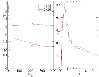
Figure 1: (Color online) Time evolution of the coarse-grained Doi-Ohta variables for a binary mixture with $\phi=0.3$, subjected to the shear flow at time $t_{0}=200t_{\rm D}$ after the beginning of a phase separating process: interfacial width $l$ (upper left), average amount of interface per unit volume $Q$ (lower left), and shear viscosity, $\eta=-q_{xy}/\dot{\gamma}$ as a function of strain $\gamma=\dot{\gamma}t$ (right). The results for the shear rates $\dot{\gamma}t_{\rm D}=0.05$ and $\dot{\gamma}t_{\rm D}=0.06$ are presented.

This numerical analysis shows that the coarse-grained Doi-Ohta variables fluctuate in time (with the time scale of $\sim 1/\dot{\gamma}$) around their average values due to the competition between the flow field and the ordering mechanisms, see Fig.1. This can be also seen in the time evolution of the morphology. The snapshots of the morphology, presented in Fig.2,

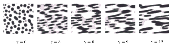
Figure 2: Configurations of a binary fluid with volume fraction $\phi=0.3$, simulated on a $128\times 128$ lattice during phase separation under shear flow at different values of strain $\gamma=\dot{\gamma}t$. Shear flow was applied after initial time of $t_{0}=200t_{\rm D}$, with the shear rate $\dot{\gamma}t_{\rm D}=0.05$. The snapshots were taken until the maximum strain $\gamma=12$. The gray scale is used in order to capture the processes of interface deformation.

show that at first domains are elongated due to the shear flow, which tends to orient them towards the shear direction. The elongation is then followed by coagulation, break-up, shape relaxation, as well as the evaporation-condensation of the droplets, which are exactly the mechanisms of interfacial relaxation proposed by Doi and Ohta DoiOhta_91 , and Lee and Park LeePark_94 . Similar interfacial relaxation processes have been identified in other works which report simulations of the Cahn-Hilliard model with and without hydrodynamic interaction OhtaNozDoi_90 ; CorGonLam-1 ; CorGonLam-2 ; CorGonLam-3 ; CorGonLam-4 ; Zhang_00 ; ShouChakr_00 ; NESS-1 ; NESS-2 ; NESS-3 ; Fielding_08 . The morphology time evolution shows no new processes that are fast compared to the Doi-Ohta level of description, and which would emerge as dissipation on the coarse-grained level through the Green-Kubo formula (34). Moreover, the time evolution curves of the Doi-Ohta variables in Fig. 1 are smooth without the presence of thermal fluctuations (which were not incorporated into our analysis). Since the above described mechanisms of interfaces relaxation are also the ones considered for the analysis of different growth regimes in the late stage kinetics of phase separation (see Section I), we conclude that the main dissipative contribution at the coarse-grained level arises through the averaging of the already present dissipative terms at the Cahn-Hilliard level, $M^{\rm(2)^{\prime}}$.

The relaxation of the Doi-Ohta variable $y=\{\rho,\mathbf{g},\epsilon,P,\mathbf{p},l\}$ could be expressed from the irreversible part of the GENERIC time evolution equation (10) as

$$\left.\frac{\partial y_{i}(\mathbf{r}_{1})}{\partial t}\right|_{\rm irrev} = \int_{V}d^{3}r_{2}\,M^{\rm(2)^{\prime}}_{ij}(\mathbf{r}_{1},\mathbf{r}_{2})\,\frac{\delta S^{\rm(2)}(y)}{\delta y_{j}(\mathbf{r}_{2})}.$$ (35)

In order to derive the coarse-grained friction matrix $M^{\rm(2)^{\prime}}$, we note that the Cahn-Hilliard friction matrix $M^{\rm(1)}$ consists of a hydrodynamic and a diffusive part, $M^{\rm(1)}=M^{\rm(1),hyd}+M^{\rm(1),dif}$, given in subsection II.1. Therefore $M^{\rm(2)^{\prime}}$ will also comprise the hydrodynamic part and a part arising from the diffusion. Since the hydrodynamic variables are simply taken over from the Cahn-Hilliard level, the appropriate hydrodynamic elements of the new friction matrix are the same as in (15). The diffusive part, on the other hand, is related to the configurational variable $c$, and the ensemble averaging must be performed in a similar way as for the Poisson operator in Section III.4. For the analytical derivation of the coarse-grained friction matrix $M^{\rm(2)^{\prime},dif}$, in analogy to Eq. (28), one starts from

$$M^{\rm(2)^{\prime},dif}\left(y\right)=\left\langle\left(\frac{\delta{\Pi}\left(x\right)}{\delta x}\right)^{\rm T}\cdot M^{\rm(1),dif}\left(x\right)\cdot\left(\frac{\delta{\Pi}\left(x\right)}{\delta x}\right)\right\rangle_{y},$$ (36)

and then employs similar procedure and approximations as in the derivation of the elements of the Poisson matrix $L^{\rm(2)}$ (see Appendix A). For example, the relaxation of the Doi-Ohta variable $Q$ could be expressed as an irreversible part of the GENERIC time evolution equation (35) as

$$\left.\frac{\partial Q(\mathbf{r}_{1})}{\partial t}\right|_{\rm irrev}=l(\mathbf{r}_{1})\int_{V}d^{3}r_{2}\,M^{\rm(2)^{\prime},dif}_{P\varepsilon}(\mathbf{r}_{1},\mathbf{r}_{2})\,\frac{1}{T(\mathbf{r}_{2})},$$ (37)

where we have used the approximation $\left.\left(\partial Q(\mathbf{r})/\partial t\right)\right|_{irrev}\approx l(\mathbf{r})\left.\left(\partial P(\mathbf{r})/\partial t\right)\right|_{irrev}$, since the interfacial width $l$ does not change much, compared to the other two configurational variables. Using the entropy functional derivative (27) with $\bm{\lambda}=\bf{0}$, results in the matrix element $M^{\rm(2)^{\prime},dif}_{P\varepsilon}$ being the only relevant term for the variable $P$ which is left after the averaging (36). Then, putting the equation (37) in the Doi-Ohta equation (7a) for the relaxation of $Q$ in a homogeneous case gives the following expression for the relaxation time

$$\frac{1}{\tau_{\rm do,1}} = \frac{2\kappa_{\rm E}Ml}{VQ}\,\int\mathcal{D}c\,\rho_{(Q,\mathbf{q})}[c]\,\int_{V}d^{3}r\,\left[\frac{\partial}{\partial\mathbf{r}}\left(\frac{\partial^{2}c(\mathbf{r})}{\partial\mathbf{r}^{2}}\right)\right]^{2},$$ (38)

where $V$ is the volume of the system. Details of the calculation are given in Appendix B. Similar expression could be obtained for the relaxation time $\tau_{\rm do,2}$. The above formula, gives the expression for the Doi-Ohta relaxation time $\tau_{\rm do,1}$ calculated from the transformation of the element of the friction matrix $M^{\rm(1),dif}$ containing the relaxation parameters of the Cahn-Hilliard level at any time $t$. This is the result of the presented systematic coarse-graining procedure developed within the GENERIC formalism which shows in which way the Doi-Ohta relaxation times can be obtained from the more detailed level of description. However, the above relation is difficult to express analytically in form of the variables of the Doi-Ohta level, due to the diffusive terms coming from the Cahn-Hilliard level. On the other hand, the above expression could, in principle, be calculated numerically using short time simulations at the Cahn-Hilliard level. However, the problems concerning the third order derivatives of the composition field $c$ make this task rather complicated, as well as the need for determination of the Lagrange multipliers in order to employ the full GENERIC procedure developed in this paper.

IV Conclusions and perspectives

In this paper, we have developed a systematic, thermodynamically guided method which establishes the coarse-grained Doi-Ohta model, used for rheological behavior, from the more detailed Cahn-Hilliard model of a phase separating binary fluid. The main contributions of the present work can be summarized as: $(1)$ the introduction of the average interfacial width $l$ as an additional structural variable; $(2)$ the derivation of the coarse-grained Poisson operator $L^{\rm(2)}$, Eq.(28), from its finer level analogue; $(3)$ no new dissipative processes arise during level jumping apart from the known hydrodynamic and diffusive dissipation; $(4)$ the derivation of an expression (38) for the Doi-Ohta relaxation times as a function of the elements of the friction matrix describing relaxation at the finer Cahn-Hilliard level.

The crucial step in the coarse-graining procedure was to identify the relevant coarse-grained variables and find the appropriate mapping which expresses them in terms of the more microscopic variables. In order to capture the physics of the Doi-Ohta level, we introduced the interfacial width $l(\mathbf{r},t)$ as an additional variable in the new model. In that way we could account for the stretching of the interface under flow and derive analytically the reversible (convective) behavior of the variables $Q(\mathbf{r},t)$ and $\mathbf{q}(\mathbf{r},t)$, which recovers the already established phenomenological Doi-Ohta model. Introduction of the interfacial width $l$ and its time evolution equation, as an addition to $Q$ and $\mathbf{q}$ of the original Doi-Ohta model with zero-width interface, offers new possibilities for modeling of the rheological behavior of multiphase flows. In addition, the expression for the interfacial tension (25) in terms of the Cahn-Hilliard parameters follows as the direct result of the developed systematic coarse-graining procedure.

Considering the irreversible dynamics on the Doi-Ohta level, it has been shown that the dissipative processes at this coarse-grained level are carried on from the more microscopic Cahn-Hilliard level. Although their analytical derivation is too complex and rich in structure, the way to connect the interface relaxation times of the Doi-Ohta model and the underlying morphology dynamics simulated at the Cahn-Hilliard level is established. Analysis of the numerical investigation of phase separation under shear in the diffusive regime revealed no new physical process that occur at the time scale which is slow compared to the Cahn-Hilliard level and fast from the perspective of the Doi-Ohta level. Therefore, there are no new dissipative effects arising in the performed coarse-graining step through the Green-Kubo type formula, i.e., no new physics appear. That leads us to the conclusion that all the dissipation has been introduced into the model by coarse graining from the reversible atomistic level to the Cahn-Hilliard level. This coarse-graining step has been done in the derivation of the hydrodynamic equations of a phase separating fluid mixture from the underlying microscopic dynamics EspTh_03 . Furthermore, Espańol and Vázquez showed in Esp_02 that all dissipation is introduced already at the very first coarse-graining step, going from the atomistic to the Fokker-Planck level. From there then follows the conclusion that the Cahn-Hilliard level is not so fundamental considering that the same dissipation mechanisms occur even at the finer levels, and are afterwards transmitted to an even more coarse-grained Doi-Ohta level, with no new dissipative processes arising.

The presented results could be used to deal with several interesting open problems. First, possible extension of the procedure to more complicated phase separating systems with the addition of surfactants or block copolymers would be very interesting for wider use. Second, the nature of the dissipative processes in a phase separating binary mixture is still far from clear. While during the diffusive regime, in the absence of thermal noise, we do not recognize any further fast processes that could be considered as fluctuations at the Doi-Ohta level, this becomes far from evident during the late stages of coarsening when inertia becomes important. The nature of the domain coarsening in the inertial hydrodynamics regime is still unknown, as well as the asymptotic behavior of a phase separating system under shear. Furthermore, recent studies showed that a nonequilibrium steady state can be reached at high Reynolds numbers (low shear rates) only in the mixed viscous-inertial regime, i.e., with any non-zero amount of inertia NESS-1 ; NESS-2 ; NESS-3 ; Fielding_08 . The fact that no steady state could be formed without presence of inertia, no matter how small, suggests that inertia plays the role of a singular perturbation in this problem Fielding_08 . The formed steady state, arising from a cyclic occurrence of elongation of domains followed by their break up, coagulation and shape relaxation, is characterized by irregular fluctuations around the attained steady state values. It would be interesting to understand the nonequilibrium steady state and the origin of these fluctuations, using the presented coarse-graining procedure. However, the phenomenological Doi-Ohta theory assumes low Reynolds number, i.e., neglects inertia. Deeper insight into the mixed viscous-inertial regime is therefore crucial in order to develop the connection between the two levels and to understand the role of inertia in this problem.

Appendix A

We present a derivation of the elements $L^{\rm(2)}_{P\mathbf{g}}(\mathbf{r}_{1},\mathbf{r}_{2})$ and $L^{\rm(2)}_{l\mathbf{g}}(\mathbf{r}_{1},\mathbf{r}_{2})$ of the coarse-grained Poisson operator $L^{\rm(2)}$ in detail. For the element $L^{\rm(2)}_{P\mathbf{g}}(\mathbf{r}_{1},\mathbf{r}_{2})$ the general expression (29) gives

$$L^{\rm(2)}_{P\mathbf{g}}(\mathbf{r}_{1},\mathbf{r}_{2}) = \int\mathcal{D}x\,\rho_{y}[x]\,\int_{V}d^{3}r_{1}^{\prime}\,\int_{V}d^{3}r_{2}^{\prime}\,\chi(\mathbf{r}_{1}-\mathbf{r}_{1}^{\prime})\,\chi(\mathbf{r}_{2}-\mathbf{r}_{2}^{\prime})$$ (39)

$$\times\int_{V}d^{3}r_{3}\,\int_{V}d^{3}r_{4}\,\frac{\delta\Pi_{P}[c](\mathbf{r}_{1}^{\prime})}{\delta c(\mathbf{r}_{3})}L^{\rm(1)}_{c\mathbf{g}}(\mathbf{r}_{3},\mathbf{r}_{4})\frac{\delta\bm{\Pi}_{\mathbf{g}}[\mathbf{g}](\mathbf{r}_{2}^{\prime})}{\delta\mathbf{g}(\mathbf{r}_{4})},$$

which after substitution of the appropriate functional derivatives, $L^{\rm(1)}_{c\mathbf{g}}$ element, and the integration over $\mathbf{r}_{3}$ and $\mathbf{r}_{4}$ becomes

$$L^{\rm(2)}_{P\mathbf{g}}(\mathbf{r}_{1},\mathbf{r}_{2}) = \int\mathcal{D}c\,\rho_{(Q,\mathbf{q})}[c]\,\int_{V}d^{3}r_{1}^{\prime}\,\int_{V}d^{3}r_{2}^{\prime}\,\chi(\mathbf{r}_{1}-\mathbf{r}_{1}^{\prime})\,\chi(\mathbf{r}_{2}-\mathbf{r}_{2}^{\prime})$$ (40)

$$\times\frac{\partial c}{\partial\mathbf{r}_{2}^{\prime}}\;\frac{\partial}{\partial\mathbf{r}_{2}^{\prime}}\cdot\left(2\,\frac{\partial c}{\partial\mathbf{r}_{2}^{\prime}}\,\chi(\mathbf{r}_{1}^{\prime}-\mathbf{r}_{2}^{\prime})\right).$$

For further calculations, we use the difference between the Cahn-Hilliard and Doi-Ohta length scales (19), so that $\int_{V}d^{3}r_{1}^{\prime}\,\chi(\mathbf{r}_{1}-\mathbf{r}_{1}^{\prime})\chi(\mathbf{r}_{1}^{\prime}-\mathbf{r}_{2}^{\prime})\approx\chi(\mathbf{r}_{1}-\mathbf{r}_{2}^{\prime})$ (see Jelic_09 ). Then the last equation, after integration over $\mathbf{r}_{1}^{\prime}$, becomes

$$L^{\rm(2)}_{P\mathbf{g}}(\mathbf{r}_{1},\mathbf{r}_{2})=\int\mathcal{D}c\,\rho_{(Q,\mathbf{q})}[c]\,\int_{V}d^{3}r_{2}^{\prime}\,\,\chi(\mathbf{r}_{2}-\mathbf{r}_{2}^{\prime})\frac{\partial c}{\partial\mathbf{r}_{2}^{\prime}}\;\frac{\partial}{\partial\mathbf{r}_{2}^{\prime}}\cdot\left(2\,\frac{\partial c}{\partial\mathbf{r}_{2}^{\prime}}\,\chi(\mathbf{r}_{1}-\mathbf{r}_{2}^{\prime})\right).$$ (41)

After integration by parts, in which surface terms vanish, using approximation $\chi(\mathbf{r}_{1}-\mathbf{r}_{2}^{\prime})\chi(\mathbf{r}_{2}-\mathbf{r}_{2}^{\prime})\approx\chi(\mathbf{r}_{1}-\mathbf{r}_{2})\chi(\mathbf{r}_{2}-\mathbf{r}_{2}^{\prime})$ valid due to the fact that the smoothing length is much smaller than the Doi-Ohta length scale, equation (19), and the identity $\partial\chi(\mathbf{r}-\mathbf{r^{\prime}})/\partial\mathbf{r^{\prime}}=-\partial\chi(\mathbf{r}-\mathbf{r^{\prime}})/\partial\mathbf{r}$, we come to the expression

$$L^{\rm(2)}_{P\mathbf{g},\beta}(\mathbf{r}_{1},\mathbf{r}_{2}) = \int\mathcal{D}c\,\rho_{(Q,\mathbf{q})}[c]\,\times\left\{\frac{\partial}{\partial r_{2\alpha}}\int_{V}d^{3}r_{2}^{\prime}\,\,2\,\frac{\partial c}{\partial r^{\prime}_{2\alpha}}\,\frac{\partial c}{\partial r^{\prime}_{2\beta}}\,\chi(\mathbf{r}_{1}-\mathbf{r}_{2})\chi(\mathbf{r}_{2}-\mathbf{r}_{2}^{\prime})\right.$$ (42)

$$-\frac{\partial}{\partial r_{1\beta}}\int_{V}d^{3}r_{2}^{\prime}\,\,\left|\nabla c(\mathbf{r}_{2}^{\prime})\right|^{2}\chi(\mathbf{r}_{1}-\mathbf{r}_{2})\chi(\mathbf{r}_{2}-\mathbf{r}_{2}^{\prime})$$

$$\left.-\frac{\partial}{\partial r_{2\beta}}\int_{V}d^{3}r_{2}^{\prime}\,\,\left|\nabla c(\mathbf{r}_{2}^{\prime})\right|^{2}\chi(\mathbf{r}_{1}-\mathbf{r}_{2})\chi(\mathbf{r}_{2}-\mathbf{r}_{2}^{\prime})\right\}.$$

Finally, with the help of the mappings (21), we can recognize the appropriate terms in the last equation, so that their ensemble average gives

$$L^{\rm(2)}_{P\mathbf{g},\beta}(\mathbf{r}_{1},\mathbf{r}_{2})=\frac{\partial}{\partial r_{2\alpha}}\left[\left(2p_{\alpha\beta}(\mathbf{r}_{2})-\frac{1}{3}P(\mathbf{r}_{2})\delta_{\alpha\beta}\right)\chi(\mathbf{r}_{1}-\mathbf{r}_{2})\right]+P(\mathbf{r}_{2})\frac{\partial\chi(\mathbf{r}_{1}-\mathbf{r}_{2})}{\partial r_{2\beta}}.$$ (43)

The Poisson operator element $L^{\rm(2)}_{l\mathbf{g}}(\mathbf{r}_{1},\mathbf{r}_{2})$ is obtained under similar approximations as above, but also the following approximations

$$\int_{V}d^{3}r_{1}^{\prime}\,\Phi[c](\mathbf{r}_{1}^{\prime})\,\chi(\mathbf{r}_{1}-\mathbf{r}_{1}^{\prime})\,\chi(\mathbf{r}_{1}^{\prime}-\mathbf{r}_{2}^{\prime})\approx\Phi[c](\mathbf{r}_{1})\,\chi(\mathbf{r}_{1}-\mathbf{r}_{2}^{\prime}),$$ (44)

which holds under the assumption of the difference in length scales (19), and the assumption

$$\left\langle\left(\Pi_{P}[c](\mathbf{r})\right)^{n}\Pi_{l}[c](\mathbf{r})\right\rangle\approx\left(\left\langle\Pi_{P}[c](\mathbf{r})\right\rangle\right)^{n}\left\langle\Pi_{l}[c](\mathbf{r})\right\rangle,$$ (45)

for $n=\pm 1$. For the element $L^{\rm(2)}_{l\mathbf{g}}(\mathbf{r}_{1},\mathbf{r}_{2})$, we then obtain

$$L^{\rm(2)}_{l\mathbf{g},\beta}(\mathbf{r}_{1},\mathbf{r}_{2}) = \frac{1}{P(\mathbf{r}_{1})}\left\langle\int_{V}d^{3}r^{\prime}\,\,\frac{\partial c}{\partial r^{\prime}_{\alpha}}\frac{\partial c}{\partial r^{\prime}_{\beta}}\left|\nabla c(\mathbf{r^{\prime}})\right|^{-1}\chi(\mathbf{r}_{1}-\mathbf{r^{\prime}})\right\rangle\frac{\partial\chi(\mathbf{r}_{1}-\mathbf{r}_{2})}{\partial r_{2\alpha}}$$ (46)

$$-\frac{\partial l(\mathbf{r}_{1})}{\partial r_{1\beta}}\chi(\mathbf{r}_{1}-\mathbf{r}_{2})-\frac{2}{3}l(\mathbf{r}_{1})\frac{\partial\chi(\mathbf{r}_{1}-\mathbf{r}_{2})}{\partial r_{2\beta}}$$

$$-2\,\frac{l(\mathbf{r}_{1})}{P(\mathbf{r}_{1})}p_{\alpha\beta}(\mathbf{r}_{1})\frac{\partial\chi(\mathbf{r}_{1}-\mathbf{r}_{2})}{\partial r_{2\alpha}}.$$

In order to express the previous equation in terms of the coarse-grained Doi-Ohta variables $\{P,\mathbf{p},l\}$, we must use the following closure approximation for the first term on the right hand side

$$\displaystyle\left\langle\int_{V}d^{3}r^{\prime}\,\,\frac{\partial c}{\partial r^{\prime}_{\alpha}}\frac{\partial c}{\partial r^{\prime}_{\beta}}\left|\nabla c(\mathbf{r^{\prime}})\right|^{-1}\chi(\mathbf{r}_{1}-\mathbf{r^{\prime}})\right\rangle\approx$$

$$\displaystyle C\left\langle\int_{V}d^{3}r^{\prime}\,\,\frac{\partial c}{\partial r^{\prime}_{\alpha}}\frac{\partial c}{\partial r^{\prime}_{\beta}}\chi(\mathbf{r}_{1}-\mathbf{r^{\prime}})\right\rangle\left\langle\int_{V}d^{3}r^{\prime}\,\,\left|\nabla c(\mathbf{r^{\prime}})\right|\chi(\mathbf{r}_{1}-\mathbf{r^{\prime}})\right\rangle\,,$$ (47)

where $C$ is chosen in such a way that the previous expression is valid when its trace is taken. By putting $\alpha=\beta$ into the above equation, we find

$$C=\left\langle\int_{V}d^{3}r^{\prime}\,\,\left|\nabla c(\mathbf{r^{\prime}})\right|^{2}\chi(\mathbf{r}_{1}-\mathbf{r^{\prime}})\right\rangle^{-1}.$$ (48)

Using the above expressions, element $L^{\rm(2)}_{l\mathbf{g}}(\mathbf{r}_{1},\mathbf{r}_{2})$ takes the final form

$$L^{\rm(2)}_{l\mathbf{g},\beta}(\mathbf{r}_{1},\mathbf{r}_{2}) = -\frac{l(\mathbf{r}_{1})}{P(\mathbf{r}_{1})}p_{\alpha\beta}(\mathbf{r}_{1})\frac{\partial\chi(\mathbf{r}_{1}-\mathbf{r}_{2})}{\partial r_{2\alpha}}-\frac{1}{3}l(\mathbf{r}_{1})\frac{\partial\chi(\mathbf{r}_{1}-\mathbf{r}_{2})}{\partial r_{2\beta}}$$ (49)

$$-\frac{\partial l(\mathbf{r}_{1})}{\partial r_{1\beta}}\chi(\mathbf{r}_{1}-\mathbf{r}_{2}).$$

Appendix B

We present the derivation of the expression (38) for the time relaxation $\tau_{\rm do,1}$. Substitution of the equation (37) for the irreversible time evolution of the configurational variable $Q$ into the Doi-Ohta relaxation equation (7a) gives

$$\frac{1}{\tau_{\rm do,1}} = -\frac{l(\mathbf{r}_{1})}{Q(\mathbf{r}_{1})}\int_{V}d^{3}r_{2}\,M^{\rm(2)^{\prime},dif}_{P\varepsilon}(\mathbf{r}_{1},\mathbf{r}_{2})\,\frac{1}{T(\mathbf{r}_{2})}\,.$$ (50)

Under the assumption of a homogeneous system, integration over the whole system size of the above expression gives

$$\frac{1}{\tau_{\rm do,1}} = -\frac{l}{QVT}\int_{V}d^{3}r_{1}\,\int_{V}d^{3}r_{2}\,M^{\rm(2)^{\prime},dif}_{P\varepsilon}(\mathbf{r}_{1},\mathbf{r}_{2})\,.$$ (51)

The general expression (36) for the coarse-grained friction matrix $M^{\rm(2)^{\prime},dif}$ gives

$$M^{\rm(2)^{\prime},dif}_{P\varepsilon}(\mathbf{r}_{1},\mathbf{r}_{2}) = \int\mathcal{D}x\,\rho_{y}[x]\,\int_{V}d^{3}r_{1}^{\prime}\,\int_{V}d^{3}r_{2}^{\prime}\,\chi(\mathbf{r}_{1}-\mathbf{r}_{1}^{\prime})\,\chi(\mathbf{r}_{2}-\mathbf{r}_{2}^{\prime})$$ (52)

$$\times\int_{V}d^{3}r_{3}\,\int_{V}d^{3}r_{4}\,\frac{\delta\Pi_{P}[c](\mathbf{r}_{1}^{\prime})}{\delta c(\mathbf{r}_{3})}M^{\rm(1),dif}_{c\epsilon}(\mathbf{r}_{3},\mathbf{r}_{4})\frac{\delta{\Pi}_{\epsilon}[\epsilon](\mathbf{r}_{2}^{\prime})}{\delta\epsilon(\mathbf{r}_{4})},$$

which after substitution of the appropriate functional derivatives, $M^{\rm(1),dif}$ element, and the integration over $\mathbf{r}_{4}$, $\mathbf{r}_{1}^{\prime}$, and $\mathbf{r}_{2}^{\prime}$ becomes

$$M^{\rm(2)^{\prime},dif}_{P\varepsilon}(\mathbf{r}_{1},\mathbf{r}_{2}) = \int\mathcal{D}c\,\rho_{(Q,\mathbf{q})}[c]\,\int_{V}d^{3}r^{\prime}\,\,2\kappa_{\rm E}MT\frac{\partial}{\partial r^{\prime}_{\alpha}}\left(\left(\frac{\partial^{2}c}{\partial\mathbf{r^{\prime}}^{2}}\right)\chi(\mathbf{r}_{2}-\mathbf{r^{\prime}})\right)$$ (53)

$$\times\frac{\partial^{2}}{\partial r^{\prime}_{\alpha}\partial r^{\prime}_{\beta}}\left(\frac{\partial c}{\partial r^{\prime}_{\beta}}\chi(\mathbf{r}_{1}-\mathbf{r^{\prime}})\right)\,,$$

where we have used the assumption of a homogeneous ($M=const.$) and isothermal system, as well as the approximations based on a difference between the Cahn-Hilliard and Doi-Ohta length scales, as in Appendix A. Substitution of the friction matrix element (53) into equation (51), gives after using the normalization condition $\int_{V}d^{3}r^{\prime}\,\,\chi(\mathbf{r}-\mathbf{r^{\prime}})=1$, the final formula for the Doi-Ohta time relaxation

$$\frac{1}{\tau_{\rm do,1}} = \frac{2\kappa_{\rm E}Ml}{VQ}\,\int\mathcal{D}c\,\rho_{(Q,\mathbf{q})}[c]\,\int_{V}d^{3}r\,\left[\frac{\partial}{\partial\mathbf{r}}\left(\frac{\partial^{2}c(\mathbf{r})}{\partial\mathbf{r}^{2}}\right)\right]^{2}.$$ (54)

References

- (1) R. G. Larson, The Structure and Rheology of Complex Fluids (Oxford University Press, New York, 1999).
- (2) S. T. Hyde and G. E. Schroder, Curr. Opin. Coll. Int. Sci. 8, 5 (2003).
- (3) C. J. Drummond and C. Fong, Curr. Opin. Coll. Int. Sci. 4, 449 (2000).
- (4) M. Caffrey, Curr. Opin. Sruct. Biol. 10, 486 (2000).
- (5) A. J. Bray, Adv. Phys. 43, 357 (1994).
- (6) A. Onuki, J. Phys.: Condens. Matter 9, 6119 (1997).
- (7) A. H. Krall, J. V. Sengers, and K. Hamano, Phys. Rev. Lett. 69, 1963 (1992).
- (8) J. Läuger, C. Laubner, and W. Gronski, Phys. Rev. Lett. 75, 3576 (1995).
- (9) K. Matsuzaka, T. Koga, and T. Hashimoto, Phys. Rev. Lett. 80, 5441 (1998).
- (10) D. Derks, D. G. A. Aarts, D. Bonn, and A. Imhof, J. Phys.: Condens. Matter 20, 404208 (2008).
- (11) D. G. A. Aarts, R. P. .A. Dullens, and H. N. W. Lekkerkerker, New J. Phys. 7, 40 (2005).
- (12) T. Ohta, H. Nozaki, and M. Doi, J. Chem. Phys. 93, 2664 (1990).
- (13) P. Padilla, and S. Toxvaerd, J. Chem. Phys. 106, 2342 (1997).
- (14) F. Corberi, G. Gonnella, and A. Lamura, Phys. Rev. Lett. 81, 3852 (1998).
- (15) F. Corberi, G. Gonnella, and A. Lamura, Phys. Rev. Lett. 83, 4057 (1999).
- (16) F. Corberi, G. Gonnella, and A. Lamura, Phys. Rev. E 61, 6621 (2000).
- (17) F. Corberi, G. Gonnella, and A. Lamura, Phys. Rev. E 62, 8064 (2000).
- (18) Z. L. Zhang, H. D. Zhang, and Y. L. Yang, J. Chem. Phys. 113, 8348 (2000).
- (19) L. Berthier, Phys. Rev. E 63, 051503 (2001).
- (20) Z. Y. Shou, and A. Chakrabarti, Phys. Rev. E 61, R2200 (2000).
- (21) A. J. Wagner and J. M. Yeomans, Phys. Rev. E 59, 4366 (1999).
- (22) P. Stansell, K. Stratford, J. C. Desplat, R. Adhikari, and M. E. Cates, Phys. Rev. Lett. 96, 085701 (2006).
- (23) K. Stratford, J. C. Desplat, P. Stansell, and M. E. Cates, Phys. Rev. E 76, 030501(R) (2007).
- (24) S. M. Fielding, Phys. Rev. E 77, 021504 (2008).
- (25) A. Onuki, Phys. Rev. A 35, 5149 (1987).
- (26) N. P. Rapapa and A. J. Bray, Phys. Rev. Lett. 83, 3856 (1999).
- (27) N. P. Rapapa, Phys. Rev. E 61, 247 (2000).
- (28) M. Doi and T. Ohta, J. Chem. Phys. 95, 1242 (1991).
- (29) J. W. Cahn and J. E. Hilliard, J. Chem. Phys. 28, 258 (1958).
- (30) P. C. Hohenberg and B. I. Halperin, Rev. Mod. Phys. 49, 435 (1977).
- (31) E. D. Siggia, Phys. Rev. A 20, 595 (1979).
- (32) H. Furukawa, Adv. Phys. 34, 703 (1985).
- (33) N. J. Wagner, H. C. Öttinger, and B. J. Edwards, AIChE J. 45, 1169 (1999).
- (34) H. M. Lee and O. O. Park, J. Rheol. 38, 1405 (1994).
- (35) M. Grmela and A. Ait-Kadi, J. Non-Newtonian Fluid Mech. 77, 191 (1998).
- (36) M. Grmela, A. Ait-Kadi, and L. A. Utracki, J. Non-Newtonian Fluid Mech. 77, 253 (1998).
- (37) C. Lacroix, M. Grmela, and P. J. Carreau, J. Rheol. 42, 41 (1998).
- (38) M. Bousmina, M. Aouina, B. Chaudhry, R. Guenette, and R. E. S. Bretas, Rheol. Acta 40, 538 (2001).
- (39) I. Vinckier and H. M. Laun, J. Rheol. 45, 1373 (2001).
- (40) J. F. Gu and Miroslav Grmela, Phys. Rev. E 78, 056302 (2008).
- (41) H. C. Öttinger, Beyond Equilibrium Thermodynamics (Wiley, Hoboken, N.J., 2005).
- (42) M. Grmela and H. C. Öttinger, Phys. Rev. E 56, 6620 (1997).
- (43) H. C. Öttinger and M. Grmela, Phys. Rev. E 56, 6633 (1997).
- (44) A. Onuki, Phys. Rev. Lett. 94, 054501 (2005).
- (45) A. Jelić, PhD thesis (ETH Zurich, Switzerland, 2009).
- (46) P. Español and C. Thieulot, J. Chem. Phys. 118, 9109 (2003).
- (47) H. C. Öttinger, MRS Bulletin 32, 936 (2007).
- (48) P. Ilg, H. C. Öttinger and M. Kröger, Phys. Rev. E 79, 011802 (2009).
- (49) V. G. Mavrantzas and H. C. Öttinger, Macromolecules 35, 960 (2002).
- (50) P. Español and F. Vázquez, Phil. Trans. R. Soc. Lond. A 360, 383 (2002).