Relativistic aspects of rotational motion of celestial bodies

Abstract

Relativistic modelling of rotational motion of extended bodies represents one of the most complicated problems of Applied Relativity. The relativistic reference systems of IAU (2000) give a suitable theoretical framework for such a modelling. Recent developments in the post-Newtonian theory of Earth rotation in the limit of rigidly rotating multipoles are reported below. All components of the theory are summarized and the results are demonstrated. The experience with the relativistic Earth rotation theory can be directly applied to model the rotational motion of other celestial bodies. The high-precision theories of rotation of the Moon, Mars and Mercury can be expected to be of interest in the near future.

1 Earth rotation and relativity

Earth rotation is the only astronomical phenomenon which is observed with very high accuracy, but is traditionally modelled in a Newtonian way. Although a number of attempts to estimate and calculate the relativistic effects in Earth rotation have been undertaken (e.g., Bizouard et al. (1992); Brumberg & Simon (2007) and reference therein) no consistent theory has appeared until now. As a result the calculations of different authors substantially differ from each other. Even the way geodetic precession/nutation is usually taken into account is just a first-order approximation and is not fully consistent with relativity. On the other hand, the relativistic effects in Earth’s rotation are relatively large. For example, the geodetic precession (1.9^′′ per century) is about $3\times 10^{-4}$ of general precession. The geodetic nutation (up to 200 $\mu$as) is 200 times larger than the goal accuracy of modern theories of Earth rotation. One more reason to carefully investigate relativistic effects in Earth rotation is the fact that the geodynamical observations yield important tests of general relativity (e.g., the best estimate of the PPN $\gamma$ using large range of angular distances from the Sun comes from geodetic VLBI data) and it is dangerous to risk that these tests are biased because of a relativistically flawed theory of Earth rotation.

Early attempts to model rotational motion of the Earth in a relativistic framework (see, for example, Brumberg 1972) made use of only one relativistic references system to describe both rotational and translational motions. That reference system was usually chosen to be quite similar to the BCRS. This resulted in a mathematically correct, but physically inadequate coordinate picture of rotational motion. For example, from that coordinate picture a prediction of seasonal LOD-variations with an amplitude of about 75 microseconds has been put forward.

At the end of the 1980s a better reference system for modelling of Earth rotation has been constructed, that after a number of modifications and improvements has been adopted as GCRS in the IAU 2000 Resolutions. The GCRS implements the Einstein’s equivalence principle and represents a reference system in which the gravitational influence of external matter (the Moon, the Sun, planets, etc.) is reduced to tidal potentials. Thus, for physical phenomena occurring in the vicinity of the Earth the GCRS represents a reference system, the coordinates of which are, in a sense, as close as possible to measurable quantities. This substantially simplifies the interpretation of the coordinate description of physical phenomena localized in the vicinity of the Earth. One important application of the GCRS is modelling of Earth rotation. The price to pay when using GCRS is that one should deal not only with one relativistic reference system, but with several reference systems, the most important of which are the BCRS and the GCRS. This makes it necessary to clearly and carefully distinguish between parameters and quantities defined in the GCRS and those defined in the BCRS.

2 Relativistic equations of Earth rotation

The model which is used in this investigation was discussed and published by Klioner et al. (2001). Let us, however, repeat these equations once again not going into physical details. The post-Newtonian equations of motion (omitting numerically negligible terms as explained in Klioner et al. (2001)) read

$${d\over dT}\,\left(C^{ab}\,\omega^{b}\right) = \sum_{l=1}^{\infty}\ {1\over l!}\ \varepsilon_{abc}\,M_{bL}\,G_{cL}+L^{a}(\mbox{\boldmath$C$},\mbox{\boldmath$\omega$},\mbox{\boldmath$\Omega$}_{\rm iner}),$$ (1)

where $T={\rm TCG}$, $\mbox{\boldmath$C$}=C^{ab}$ is the post-Newtonian tensor of inertia and $\mbox{\boldmath$\omega$}=\omega^{a}$ is the angular velocity of the post-Newtonian Tisserand axes (Klioner 1996), $M_{L}$ are the multipole moments of the Earth’s gravitational field defined in the GCRS, $G_{L}$ are the multipole moments of the external tidal gravito-electric field in the GCRS. In the simplest situation (a number of mass monopoles) $G_{L}$ are explicitly given by Eqs. (19)–(23) of Klioner et al. (2001).

The additional torque $L^{a}$ depends on $C$, $\omega$, as well as on the angular velocity $\mbox{\boldmath$\Omega$}_{\rm iner}$ describing the relativistic precessions (geodetic, Lense-Thirring and Thomas precessions). The definition of $\mbox{\boldmath$\Omega$}_{\rm iner}$ can be found, e.g., in Klioner et al. (2001). A detailed discussion of $L^{a}$, its structure and consequences will be published elsewhere (Klioner et al. 2009).

The model of rigidly rotating multipoles (Klioner et al. 2001) represents a set of formal mathematical assumptions that make the general mathematical structure of Eqs. (1) similar to that of the Newtonian equations of rotation of a rigid body:

$$C^{ab} = P^{ac}\,P^{bd}\,{\overline{C}}^{cd},\quad{\overline{C}}^{cd}={\rm const}$$ (2)

$$M_{a_{1}a_{2}\dots a_{l}} = P^{a_{1}b_{1}}\,P^{a_{2}b_{2}}\dots P^{a_{l}b_{l}}\,{\overline{M}}_{b_{1}b_{2}\dots b_{l}},\quad{\overline{M}}_{b_{1}b_{2}\dots b_{l}}={\rm const},\quad l\geq 2,$$ (3)

where the orthogonal matrix $P^{ab}(T)$ is assumed to be related to the angular velocity $\omega^{a}$ used in (1) as

$$\omega^{a}={1\over 2}\,\varepsilon_{abc}\,P^{db}(T)\,{d\over dT}\,P^{dc}(T).$$ (4)

The meaning of these assumptions is that both the tensor of inertia $C^{ab}$ and the multipole moments of the Earth’s gravitational field $M_{L}$ are “rotating rigidly” and that their rigid rotation is described by the same angular velocity $\omega^{a}$ that appears in the post-Newtonian equations of rotational motion. It means that in a reference system obtained from the GCRS by a time-dependent rotation of spatial axes both the tensor of inertia and the multipole moments of the Earth’s gravitational field are constant.

No acceptable definition of a physically rigid body exists in General Relativity. The model of rigidly rotating multipoles represent a minimal set of assumptions that allows one to develop the post-Newtonian theory of rotation in the same manner as one usually does within Newtonian theory for rigid bodies. In the model of rigidly rotating multipoles only those properties of Newtonian rigid bodies are saved which are indeed necessary for the theory of rotation. For example, no assumption on local physical properties (“local rigidity”) is made. It has not been proved as a theorem, but it is rather probable that no physical body can satisfy assumptions (2)–(4). The assumptions of the model of rigidly rotating multipoles will be relaxed in a later stage of the work when non-rigid effects are discussed.

3 Post-Newtonian equations of rotational motions in numerical computations

Looking at the post-Newtonian equations of motion (1)–(4) one can formulate several problems to be solved before the equations can be used in numerical calculations:

• How to parametrize the matrix $P^{ab}$?

• How to compute $M_{L}$ from the standard models of the Earth’s gravity field?

• How to compute $G_{L}$ from a solar system ephemeris?

• How to compute the torque $\varepsilon_{abc}\,M_{bL}\,G_{cL}$ out of $M_{L}$ and $G_{L}$?

• How to deal with different time scales (TCG, TCB, TT, TDB) appearing in the equations of motion, solar system ephemerides, used models of Earth gravity, etc.?

• How to treat the relativistic scaling of various parameters when using TDB and/or TT instead of TCB and TCG?

• How to find relativistically meaningful numerical values for the initial conditions and various parameters?

These questions are discussed below.

4 Relativistic definitions of the angles

One of the tricky points is the definition of the angles describing the Earth orientation in the relativistic framework. Exactly as in Bretagnon et al. (1997, 1998) we first define the rotated BCRS coordinates $(x,y,z)$ by two constant rotations of the BCRS as realized by the JPL’s DE403:

$$\left(\matrix{x\cr y\cr z}\right)=R_{x}(23^{\circ}26^{\prime}21.40928^{\prime\prime})\,R_{z}(-0.05294^{\prime\prime})\,\left(\matrix{x\cr y\cr z}\right)_{\rm DE403}.$$ (5)

Then the IAU 2000 transformations between BCRS and GCRS are applied to the coordinates $(t,x,y,z)$, $t$ being TCB, to get the corresponding GCRS coordinates $(T,X,Y,Z)$. The spatial coordinates $(X,Y,Z)$ are then rotated by the time-dependent matrix $P^{ij}$ to get the spatial coordinates of the terrestrial reference system $(\xi,\eta,\zeta)$. The matrix $P^{ij}$ is then represented as a product of three orthogonal matrices:

$$\left(\matrix{\xi\cr\eta\cr\zeta}\right)=R_{z}(\phi)\,R_{x}(\omega)\,R_{z}(\psi)\,\left(\matrix{X\cr Y\cr Z}\right).$$ (6)

The angles $\phi$, $\psi$ and $\omega$ are used to parametrize the orthogonal matrix $P^{ab}$ and therefore, to define the orientation of the Earth orientation in the GCRS. The meaning of the terrestrial system $(\xi,\eta,\zeta)$ here is the same as in Bretagnon et al. (1997): this is the reference system in which we define the harmonic expansion of the gravitational field with the standard values of potential coefficients $C_{lm}$ and $S_{lm}$.

5 STF model of the torque

The relativistic torque requires computations with symmetric and trace-free cartesian (STF) tensors $M_{L}$ and $G_{L}$. For this project special numerical algorithms for numerical calculations have been developed. The detailed algorithms and their derivation will be published elsewhere. Let us give here only the most important formulas. For each $l$ the component $D_{a}=\varepsilon_{abc}\,M_{bL-1}\,G_{cL-1}$ of the torque in the right-hand side of Eq. (1) can be computed as ($A_{l}=4\,l\,\pi\,l!/(2l+1)!!$, $a^{+}_{lm}=\sqrt{l(l+1)-m(m+1)}\$)

$$D_{1} = {1\over A_{l}}\,\Biggl{(}\sum_{m=0}^{l-1}a^{+}_{lm}\,\left(-{\cal M}^{R}_{lm}\,{\cal G}^{I}_{l,m+1}+{\cal M}^{I}_{l,m+1}\,{\cal G}^{R}_{lm}\right)$$ (7)

$$\qquad+\sum_{m=1}^{l-1}a^{+}_{lm}\,\left({\cal M}^{I}_{lm}\,{\cal G}^{R}_{l,m+1}-{\cal M}^{R}_{l,m+1}\,{\cal G}^{I}_{lm}\right)\Biggr{)},$$

$$D_{2} = {1\over A_{l}}\,\Biggl{(}\sum_{m=0}^{l-1}a^{+}_{lm}\,\left(-{\cal M}^{R}_{lm}\,{\cal G}^{R}_{l,m+1}+{\cal M}^{R}_{l,m+1}\,{\cal G}^{R}_{lm}\right)$$ (8)

$$\qquad+\sum_{m=1}^{l-1}a^{+}_{lm}\,\left(-{\cal M}^{I}_{lm}\,{\cal G}^{I}_{l,m+1}+{\cal M}^{I}_{l,m+1}\,{\cal G}^{I}_{lm}\right)\Biggr{)},$$

$$D_{3} = {2\over A_{l}}\,\sum_{m=1}^{l}\,m\left({\cal M}^{I}_{lm}\,{\cal G}^{R}_{lm}-{\cal M}^{R}_{lm}\,{\cal G}^{I}_{lm}\right).$$ (9)

The coefficients ${\cal G}^{R}_{lm}$ and ${\cal G}^{I}_{lm}$ characterizing the tidal field can be computed from Eqs. (19)–(23) of Klioner et al. (2001) as explicit functions of the parameters of the solar system bodies: their masses, positions, velocities and accelerations. A Fortran code to compute ${\cal G}^{R}_{lm}$ and ${\cal G}^{I}_{lm}$ for $l<7$ and $0\leq m\leq l$ has been generated automatically with a specially written software package for Mathematica. It is possible to develop a sort of recursive algorithm to compute ${\cal G}^{R}_{lm}$ and ${\cal G}^{I}_{lm}$ for any $l$ similar to the corresponding algorithms for, e.g., Legendre polynomials.

The coefficients ${\cal M}^{R}_{lm}$ and ${\cal M}^{I}_{lm}$ characterizing the gravitational field of the Earth can be computed as

$${\cal M}^{R}_{l0} = {l!\over(2l-1)!!}\,\left({4\pi\over 2l+1}\right)^{1/2}\,M_{E}\,R_{E}^{l}\,C_{l0},$$ (10)

$${\cal M}^{R}_{lm} = (-1)^{m}\,{1\over 2}\,{l!\over(2l-1)!!}\,\left({4\,\pi\over 2l+1}\,{(l+m)!\over(l-m)!}\right)^{1/2}\,M_{E}\,R_{E}^{l}\,C_{lm},\ 1\leq m\leq l,$$ (11)

$${\cal M}^{I}_{lm} = (-1)^{m+1}\,{1\over 2}\,{l!\over(2l-1)!!}\,\left({4\,\pi\over\,2l+1}\,{(l+m)!\over(l-m)!}\right)^{1/2}\,M_{E}\,R_{E}^{l}\,S_{lm},\ 1\leq m\leq l,$$ (12)

where $M_{E}$ is the mass of the Earth, $R_{E}$ its radius, $C_{lm}$ and $S_{lm}$ are usual potential coefficients of the Earth’s gravitational field. If only Newtonian terms are considered in the torque this formulation with STF tensors is fully equivalent to the classical formulation with Legendre polynomials (e.g., Bretagnon et al. 1997, 1998). If the relativistic terms are taken in account, the only known way to express the torque is that with STF tensors.

6 Time transformations

An important aspect of relativistic Earth rotation theory is the treatment of different relativistic time scales. The transformation between TDB and TT at the geocenter (all the transformations in this Section are meant to be “evaluated at the geocenter”) are computed along the lines of Section 3 of Klioner (2008b). Namely,

$${\rm TT}= {\rm TDB} +\Delta{\rm TDB}({\rm TDB}),$$ (13)

$${\rm TDB}= {\rm TT} -\Delta{\rm TT}({\rm TT}),$$ (14)

$${\rm TCG}= {\rm TCB} +\Delta{\rm TCB}({\rm TCB}),$$ (15)

$${\rm TCB}= {\rm TCG} -\Delta{\rm TCG}({\rm TCG}),$$ (16)

so that

$${d\Delta{\rm TDB}\over d{\rm TDB}} = A_{{\rm TDB}}+B_{{\rm TDB}}\,{d\Delta{\rm TCB}\over d{\rm TCB}},$$ (17)

$$A_{{\rm TDB}} = {L_{B}-L_{G}\over 1-L_{B}},$$ (18)

$$B_{{\rm TDB}} = {1-L_{G}\over 1-L_{B}}=A_{{\rm TDB}}+1,$$ (19)

$${d\Delta{\rm TT}\over d{\rm TT}} = A_{{\rm TT}}+B_{{\rm TT}}\,{d\Delta{\rm TCG}\over d{\rm TCG}},$$ (20)

$$A_{{\rm TT}} = {L_{B}-L_{G}\over 1-L_{G}},$$ (21)

$$B_{{\rm TT}} = {1-L_{B}\over 1-L_{G}}=1-A_{{\rm TT}},$$ (22)

$${d\Delta{\rm TCB}\over d{\rm TCB}} = F({\rm TCB})={1\over c^{2}}\,\alpha({\rm TCB})+{1\over c^{4}}\,\beta({\rm TCB}),$$ (23)

$${d\Delta{\rm TCG}\over d{\rm TCG}} = {F({\rm TCG}-\Delta{\rm TCG})\over 1+F({\rm TCG}-\Delta{\rm TCG})},$$ (24)

where the functions $\alpha$ and $\beta$ are given by Eqs. (3.3)–(3-4) of Klioner (2008b) and Eq. (24) represents a computational improvement of Eq. (3.8) of Klioner (2008b). Clearly, the derivatives $d\Delta{\rm TCB}/dTCB$ and $d\Delta{\rm TCG}/dTCG$ must be expressed as functions of TDB and TT, respectively, when used in (17)–(20).

The differential equations for $\Delta{\rm TDB}$ and $\Delta{\rm TT}$ are first integrated numerically for the whole range of the used solar system ephemeris (any ephemeris with DE-like interface can be used with the code). The initial conditions for $\Delta{\rm TDB}$ and $\Delta{\rm TT}$ are chosen according to the IAU 2006 Resolution defining TDB: for $JD_{{\rm TT}}=2443144.5003725$ one has $JD_{{\rm TDB}}=2443144.5003725-6.55\times 10^{−5}/86400$ and vice versa. The results of the integrations for the pairs $\Delta{\rm TDB}$ and $d\Delta{\rm TCB}/dTCB$, and $\Delta{\rm TT}$ and $d\Delta{\rm TT}/dTT$ are stored with a selected step in the corresponding time variable (TDB for $\Delta{\rm TDB}$ and its derivative, and TT for $\Delta{\rm TT}$ and its derivative). A cubic spline on the equidistant grid is then constructed for each of these 4 quantities. The accuracy of the spline representation is automatically estimated using additional data points computed during the numerical integration. These additional data points lie between the grid points used for the spline and are only used to control the accuracy of the spline. The splines precomputed and validated in this way are stored in files and read in by the main code upon request. These splines are directly used for time transformation during the numerical integrations of Earth rotation. Although this spline representation requires significantly more stored coefficients than, for example, a representation with Chebyshev polynomials with the same accuracy, the spline representation has been chosen because of its extremely high computational efficiency. More sophisticated representations may be implemented in future versions of the code.

7 Relativistic scaling of parameters

Obviously, there are two classes of quantities entering Eqs. (1)–(4) that are defined in the BCRS and GCRS and, therefore, naturally parametrized by TCB and TCG, respectively. It is important to realize that the post-Newtonian equations of motion are only valid if non-scaled time scales TCG and TCB are used. If TT and/or TDB are needed, the equations should be changed correspondingly.

The relevant quantities defined in the GCRS and parametrized by TCG are: (1) the orthogonal matrix $P^{ab}$ and quantities related to that matrix: angular velocity $\omega^{a}$ and corresponding Euler angles $\varphi$, $\psi$ and $\omega$; (2) the tensor of inertia $C^{ab}$; (3) the multipole moment of Earth’s gravitational field $M_{L}$. In principle, (a) $G_{L}$ and (b) $\Omega^{a}_{\rm iner}$ are also defined in the GCRS and parametrized by TCG, but these quantities are computed using positions $\mbox{\boldmath$x$}_{A}$, velocities $\mbox{\boldmath$v$}_{A}$ and accelerations $\mbox{\boldmath$a$}_{A}$ of solar system bodies. The orbital motion of solar system bodies are modelled in BCRS and parametrized by TCB or TDB. The definition of $G_{L}$ is conceived in such a way that positions, velocities and accelerations of solar system bodies in the BCRS should be taken at the moment of TCB corresponding to the required moment of TCG with spatial location taken at the geocenter. Let us recall that the transformation between TCB and TCG is a 4-dimensional one and require the spatial location of an event to be known.

In all theoretical works aimed to derive and/or analyze the rotational equations of motion in the GCRS one uses TCG as coordinate time scale parametrizing the equations. Although the natural time variable for the equations of Earth rotation is TCG, in principle, using a corresponding re-parametrization any time scale (including TCG, TT, TCB and TDB) can be used as independent time variable. Thus, simple rescaling of the first and second derivatives of the angles entering the equations of rotational motion should be applied to use TT instead of TCG:

$${d\theta\over d{\rm TCG}} = (1-L_{G})\,{d\theta\over d{\rm TT}},$$ (25)

$${d^{2}\theta\over d{\rm TCG}^{2}} = (1-L_{G})^{2}\,{d^{2}\theta\over d{\rm TT}^{2}},$$ (26)

where $\theta$ is any of the angles $\varphi$, $\psi$ and $\omega$ used in the equations of motion to parametrize the orientation of the Earth. If TDB is used as independent variable the corresponding formulas are more complicated:

$${d\theta\over d{\rm TCG}} = (1-L_{G})\,{\left(\left.{d{\rm TT}\over d{\rm TDB}}\right|_{\mbox{\boldmath$x$}_{E}}\right)}^{-1}\,{d\theta\over d{\rm TDB}},$$ (27)

$${d^{2}\theta\over d{\rm TCG}^{2}} = (1-L_{G})^{2}\,\left(\left.{d{\rm TT}\over d{\rm TDB}}\right|_{\mbox{\boldmath$x$}_{E}}\right)^{-2}\,{d^{2}\theta\over d{\rm TDB}^{2}}$$ (28)

$$-(1-L_{G})^{2}\,\left(\left.{d{\rm TT}\over d{\rm TDB}}\right|_{\mbox{\boldmath$x$}_{E}}\right)^{-3}\,\left.{d^{2}{\rm TT}\over d{\rm TDB}^{2}}\right|_{\mbox{\boldmath$x$}_{E}}\,{d\theta\over d{\rm TDB}},$$

where the derivatives of TT w.r.t. TDB should be evaluated at the geocenter (i.e., for $\mbox{\boldmath$x$}=\mbox{\boldmath$x$}_{E}$). These relations must be substituted into the equations of rotation motion to replace the derivatives of the angles $\varphi$, $\psi$ and $\omega$ w.r.t. TCG as appear e.g., in Eqs. (7)–(9) of Bretagnon et al. (1998). It is clear that the parametrization with TDB makes the equations more complicated.

The values of the parameters naturally entering the equations of rotational motion must be interpreted as unscaled (TCB-compatible or TCG-compatible) values. If scaled (TT-compatible or TDB-compatible) values are used, the scaling must be explicitly taken into account. The relativistic scaling of parameters read (see, e.g., Klioner 2008a):

$$GM_{A}^{{\rm TT}}=(1-L_{G})\,GM_{A}^{{\rm TCG}},\ GM_{A}^{{\rm TCG}}=GM_{A}^{{\rm TCB}},$$

$$\qquad\qquad\qquad\qquad\qquad\qquad\quad GM_{A}^{{\rm TDB}}=(1-L_{B})\,GM_{A}^{{\rm TCB}},$$ (29)

$$X^{{\rm TT}}=(1-L_{G})\,X^{{\rm TCG}},\ x^{{\rm TDB}}=(1-L_{B})\,x^{{\rm TCB}},$$ (30)

$$V^{{\rm TT}}=V^{{\rm TCG}},\ v^{{\rm TDB}}=v^{{\rm TCB}},$$ (31)

$$A^{{\rm TT}}=(1-L_{G})^{-1}\,A^{{\rm TCG}},\ a^{{\rm TDB}}=(1-L_{B})^{-1}\,a^{{\rm TCB}},$$ (32)

where $GM_{A}$ is the mass parameter of a body, $x$, $v$, and $a$ are parameters represents spatial coordinates (distances), velocities and accelerations in the BCRS, respectively, while $X$, $V$, and $A$ are similar quantities in the GCRS.

Now, considering the source of the numerical values of the parameters used in the equations of Earth rotation we can see the following.

• The position $\mbox{\boldmath$x$}_{A}$, velocities $\mbox{\boldmath$v$}_{A}$, accelerations $\mbox{\boldmath$a$}_{A}$ and mass parameters $GM_{A}$ of the massive solar system bodies are taken from standard JPL ephemerides and are TDB-compatible.

• The radius of the Earth comes together with the potential coefficients $C_{lm}$ and $S_{lm}$ from a model of the Earth’s gravity field (e.g., GEMT3 was used in SMART). These values come from SLR and dedicated techniques like GRACE. GCRS with TT-compatible quantities is used to process these data. Therefore, the values of the radius of the Earth is TT-compatible. Obviously, $C_{lm}$ and $S_{lm}$ have the same values when used with any time scale. The mass parameter $GM_{E}$ of the Earth coming with the Earth gravity models is also TT-compatible.

• From the definitions of ${\cal M}^{R}_{lm}$ and ${\cal M}^{I}_{lm}$ given above and formulas for $G_{L}$ given by Eqs. (19)–(23) of Klioner et al. (2001), it is easy to see that the TCG-compatible torque $F^{a}=\sum_{l=1}^{\infty}\ {1\over l!}\ \varepsilon_{abc}\,M_{bL}\,G_{cL}$ can be computed using TDB-compatible values of mass parameters $GM_{A}^{\rm TDB}$, positions $\mbox{\boldmath$x$}_{A}^{\rm TDB}$, velocities $\mbox{\boldmath$v$}_{A}^{\rm TDB}$ and accelerations $\mbox{\boldmath$a$}_{A}^{\rm TDB}$ of all external bodies, TDB-compatible value of the mass parameter of the Earth $GM_{E}^{\rm TDB}$ and the value of the Earth’s radius formally rescaled from TT to TDB as $R_{E}^{\rm TDB}=(1-L_{B})\,(1-L_{G})^{-1}\,R_{E}^{\rm TT}$. Denoting the resulting torque by $F^{a}_{\rm TDB}$, it can be seen that the TCG-compatible value is $F^{a}_{\rm TCG}=(1-L_{B})^{-1}\,F^{a}_{\rm TDB}$.

• The values of the Earth’s moments of inertia ${\cal A}_{i}$, $i=1,2,3$ can be represented as $G{\cal A}_{i}=GM_{E}R_{E}^{2}k_{i}$, where $k_{i}$ is a factor characterizing the distribution of matter inside the Earth. Clearly, the factors $k_{i}$ do not depend on the scaling. Therefore, the moments of inertia can be scaled as

  $${\cal A}_{i}^{{\rm TT}}=(1-L_{G})^{3}\,{\cal A}_{i}^{{\rm TCG}}.$$ (33)

The last question is how to interpret the values of the moments of inertia ${\cal A}_{i}=(A,B,C)$ and the initial conditions for the angles $\varphi$, $\psi$ and $\omega$ and their derivatives given in Bretagnon et al. (1998). Obviously, the initial angles at J2000 are independent of the scaling. For the other parameters in question it is not possible to clearly claim if the given values are TDB-compatible or TT-compatible. Arguments in favor of both interpretations can be given. A rigorous solution here is only possible when all calculations leading to these quantities are repeated in the framework of General Relativity. In this paper we prefer to interpret the SMART values of ${\cal A}_{i}$, $\dot{\varphi}$, $\dot{\psi}$ and $\dot{\omega}$ as being TT-compatible. Therefore, if TDB is used as independent variable, the values of the derivatives should be changed accordingly. For any of these angles one has

$${d\alpha\over d{\rm TDB}}={\left(\left.{d{\rm TT}\over d{\rm TDB}}\right|_{\mbox{\boldmath$x$}_{E}}\right)}\,{d\alpha\over d{\rm TT}}\,.$$ (34)

Thus, we have all tools to treat correctly the relativistic scaling of all relevant parameters of the Earth rotation theory as well as relativistic time scales.

8 Geodetic precession and nutation

In the framework of our model geodetic precession and nutation are taken into account in a natural way by including the additional torque that depends on $\Omega^{a}_{\rm iner}$ in the equations of rotational motion:

$$L^{a}=\varepsilon_{abc}\,C^{bd}\,\omega^{d}\,\Omega_{\rm iner}^{c}-\frac{d}{dT}\left({C^{ab}\,\Omega_{\rm iner}^{b}}\right).$$ (35)

The first term of the additional torque reflects the fact that the GCRS of the IAU is defined to be kinematically non-rotating (see Soffel et al. 2003). The second term has been usually hidden by the corresponding re-definition of the post-Newtonian spin (Damour, Soffel & Xu 1993; Klioner & Soffel 2000). It can be demonstrated that this second term must be explicitly taken into account to maintain the consistency between dynamically and kinematically non-rotating solutions. Further details will be published elsewhere (Klioner et al. 2009). Using the additional torque $L^{a}$ in Eq. (1) is a rigorous way to take geodetic precession/nutation into account.

The standard way to account for geodetic precession/nutation that was used up to now by a number of authors can be described as follows: (1) solve the purely Newtonian equations of rotational motion and consider this solution as a relativistic one in a dynamically non-rotating version of the GCRS and (2) add the precomputed geodetic precession/nutation to it. The second step is fully correct since the geodetic precession/nutation is by definition the rotation between the kinematically and dynamically non-rotating versions of the GCRS and it can be precomputed since it is fully independent of the Earth rotation. The inconsistency of the first step comes from the fact that in the computation of the Newtonian torque the coordinates of the solar system bodies are taken from an ephemeris constructed in the BCRS. However, the dynamically non-rotating version of the GCRS rotates relative to the BCRS with angular velocity $\Omega^{a}_{\rm iner}(T)$. This means that the BCRS coordinates of solar system bodies should be first rotated into “dynamically non-rotating coordinates” and only after that rotation those coordinates can be used to compute the Newtonian torque. For this reason this procedure does not lead to a correct solution in the kinematically non-rotating GCRS (see Fig. 1). We will call such solutions in this paper “SMART-like kinematical solutions”.

On the other hand, there are two ways to obtain a correct kinematically non-rotating solution: (1) use the torque given by Eq. (35) in the equations of motion, (2) compute the geodetic precession/nutation matrix, apply the geodetic precession/nutation to the solar system ephemeris, integrate (1) without $L^{a}$ with the obtained rotated ephemeris (the correct solution in a dynamically non-rotating version of the GCRS is obtained in this step), apply the geodetic precession/nutation matrix to the solution. We have implemented both ways in our code and checked explicitly that they give the same solution (to within about 0.001 $\mu$as over 150 years). It is interesting to note that the rotational matrix of geodetic precession/nutation (that is, the matrix defining a rotation with the angular velocity $\Omega_{\rm iner}^{a}$) cannot be parametrized by normal Euler angles. We have used therefore the quaternion representation for that matrix.

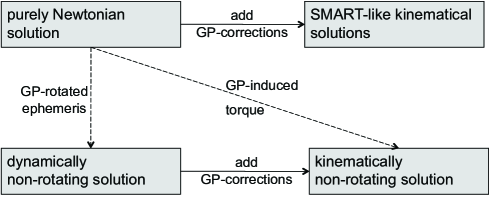
Figure 1: Scheme of the two ways to obtain a kinematically non-rotating solution from a purely Newtonian one, and an illustration of the relation between the correct kinematically non-rotating solution and SMART-like kinematical solutions. “GP” stands for geodetic precession/nutation. Each gray block represents a solution. A solid line means: add precomputed geodetic precession/nutation into a solution to get a new one. A dashed line means: recompute a solution with indicated change in the torque model.

9 Overview of the numerical code

A code in Fortran 95 has been written to integrate the post-Newtonian equations of rotational motion numerically. The software is carefully coded to avoid numerical instabilities and excessive round-off errors. Two numerical integrators with dense output – ODEX and Adams-Bashforth-Moulton multistep integrator – can be used for numerical integrations. These two integrators can be used to crosscheck each other. The integrations are automatically performed in two directions – forwards and backwards – that allows one to directly estimate the accuracy of the integration. The code is able to use any type of arithmetic available with a given current hardware and compiler. For a number of operations, which have been identified as precision-critical, one has the possibility to use either the library FMLIB Smith (2001) for arbitrary-precision arithmetic or the package DDFUN that uses two double-precision numbers to implement quadrupole-precision arithmetic (Bailey 2005). Our current baseline is to use ODEX with 80 bit arithmetic. The estimated errors of numerical integrations after 150 years of integration are below $0.001$ $\mu$as.

Several relativistic features have been incorporated into the code: (1) the full post-Newtonian torque using the STF tensor machinery, (2) rigorous treatment of geodetic precession/nutation as an additional torque in the equations of motion, (3) rigorous treatment of time scales (any of the four time scales – TT, TDB, TCB or TCG – evaluated at the geocenter can be used as the independent variable of the equations of motion (TCG being physically preferable for this role), (4) correct relativistic scaling of constants and parameters. All these “sources of relativistic effects” can be switched on and off independently of each other.

In order to test our code and the STF-tensor formulation of the torque we have coded also the classical Newtonian torque with Legendre polynomials as described by Bretagnon et al. (1997, 1998) and integrated our equations for 150 years with these two torque algorithms. Maximal deviations between these two integrations were 0.0004 $\mu$as for $\phi$, 0.0001 $\mu$as for $\psi$, and 0.0002 $\mu$as for $\omega$. This demonstrates both the equivalence of the two formulations and the correctness of our code.

We have also repeated the Newtonian dynamical solution of SMART97 using the Newtonian torque, the JPL ephemeris DE403 and the same initial values as in Bretagnon et al. (1998). Jean-Louis Simon (2007) has provided us with the unpublished full version of SMART97 (involving about 70000 Poisson terms for each of the three angles). We have calculated the differences between that full SMART97 series and our numerical integration over 150 years. Analysis of the results and a comparison to Bretagnon et al. (1998) have demonstrated that our integrations reproduce SMART97 within the full accuracy of the latter.

10 Relativistic vs. Newtonian integrations

We have performed a series of numerical calculations comparing purely Newtonian integration with integration where relativistic effects are taken into account. The same initial conditions and parameters that we used to reconstruct the SMART97 solution were used for all integrations (see below). The results are illustrated on Figs. 2–5. The difference between the kinematical SMART97 solution and the consistent kinematically-non-rotating solution obtained as described in Section 8 is shown in Fig. 2. Fig. 3 shows the effects of the post-Newtonian torque. The effects of the relativistic scaling and time scales are depicted in Fig. 4. Finally, Fig. 5 demonstrates the differences between a SMART-like kinematical solution and our full post-Newtonian integration. A detailed analysis of these results will be done elsewhere.

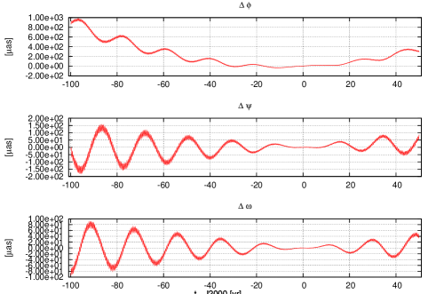
Figure 2: Differences (in $\mu$as) between the published kinematical SMART97 solution and the correct kinematically non-rotating solution (with post-Newtonian torques, relativistic scaling and time scaled neglected).

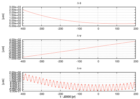
Figure 3: The effect (in $\mu$as) of the post-Newtonian torque.

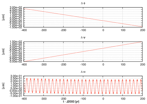
Figure 4: The effect (in $\mu$as) of the relativistic scaling and time scales.

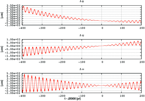
Figure 5: Difference between a purely Newtonian integration rotated for geodetic precession/nutation in a SMART-like way (see Section 8) and our solution that includes all relativistic effects discussed here.

To complete the consistent post-Newtonian theory of Earth rotation the parameters (first of all, the moments of inertia of the Earth) should be fitted to be consistent with the observed precession rate. This task will be discussed and treated in the near future.

11 Relativistic effects in rotational bodies of other bodies

The same numerical code can be applied to model the rotational motion of other bodies. Especially, high-accuracy models of rotational motion of the Moon, Mercury and Mars are of interest because of the planned space missions to Mercury and Mars, and the expected improvements of the accuracy of LLR. Most of the changes in the code are trivial and concern the numerical values of the constants. One important improvement of the code is necessary for the Moon: the figure-figure interaction with the Earth must be taken into account. Using the STF approach to compute the torque this task is not difficult.

The relativistic effects in the rotation of Moon, Mars and Mercury may be significantly larger than in the rotation of Earth. In Table 1 the amplitudes of geodetic precession and nutation are given for several solar system bodies. One can see the large effects for Mercury and Mars. Besides an early investigation of Bois & Vokroulicky (1995) suggests that the effects of the relativistic torque for the Moon may attain 1 mas. Our approach allows one to investigate the rotational motion of the Moon, Mars and Mercury in a rigorous relativistic framework.

body	geodetic precession	geodetic nutation
	[ ′′ per century ]	[ $\mu$as ]
Earth	1.92	153
Moon	1.95	154
Mercury	21.43	5080
Venus	4.32	85
Mars	0.68	567

Table 1: Magnitude of geodetic precession/nutation for various bodies

References

- Bailey (2005) Bailey, D.H., 2005, Computing in Science and Engineering, 7(3), 54;see also http://crd.lbl.gov/ dhbailey/mpdist/
- Bizouard et al. (1992) Bizouard C., Schastok, J., Soffel M.H., Souchay J., (1992) In: Journées 1992, N. Capitaine (ed.), Observatoire de Paris, 76
- Bois & Vokroulicky (1995) Bois, E., Vokrouhlicky, D., 1995, A&A, 300, 559
- Bretagnon et al. (1997) Bretagnon, P., Francou, G., Rocher, P., Simon, J.L., 1997, A&A, 319, 305
- Bretagnon et al. (1998) Bretagnon, P., Francou, G., Rocher, P., Simon, J.L., 1998, A&A, 329, 329
- Brumberg (1972) Brumberg, V.A., 1972, Relativistic Celestial Mechanics, Nauka: Moscow, in Russian
- Brumberg & Simon (2007) Brumberg, V.A., Simon, J.-L., 2007, Notes scientifique et techniques de l’insitut de méchanique céleste, S088
- Damour, Soffel & Xu (1993) Damour, T., Soffel, M., Xu, Ch., 1993, Phys. Rev. D 47, 3124
- Klioner & Voinov (1993) Klioner, S.A., Voinov, A.V., 1993, Phys. Rev. D 48, 1451
- Klioner (1996) Klioner, S.A., 1996, In: “Dynamics, Ephemerides, and Astrometry of the Solar System”, Ferraz-Mello, S. and Morando, B., Arlot, J.-E. (eds.), Proc. of IAU Symposium 172, Springer, New York, 309
- Klioner & Soffel (2000) Klioner, S.A., Soffel, M., 2000, Phys. Rev. D 62, 024019
- Klioner et al. (2001) Klioner, S.A., Soffel, M., Xu. C., Wu, X., 2001, In: Influence of geophysics, time and space reference frames on Earth rotation studies (Proc. Journées’ 2001), N. Capitaine (ed.), Paris Observatory, Paris, 232
- Klioner (2008a) Klioner, S.A., 2008a, A&A, 478, 951
- Klioner (2008b) Klioner, S.A., 2008b, In: A Giant Step: from Milli- to Micro-arcsecond Astrometry, W.Jin, I.Platais, M.Perryman (eds.) Proc. of the IAU Symposium 248, Cambridge University Press, Cambridge, 356
- Klioner et al. (2009) Klioner, S.A., Gerlach, E., Soffel, M., 2009, “Rigorous treatment of geodetic precession in the theory of Earth rotation”, in preparation
- Simon (2007) Simon, J.-L., 2007, private communication
- Smith (2001) Smith, D., 2001, “FMLIB”, http://myweb.lmu.edu/dmsmith/FMLIB.html
- Soffel et al. (2003) Soffel, M., Klioner, S.A., Petit, G. et al., 2003, Astron.J., 126, 2687