Noise and nonlinearities in high-throughput data.

Abstract

High throughput data analysis are becoming common in biology, communications, economics and sociology. This vast amount of data are usually represented in form of matrices and can be considered as knowledge networks. Spectral-based approaches have been proved useful in extracting hidden information within such networks and to estimate missing data, but these methods are based essentially on linear assumptions. The physical models of matching, when available, often suggest nonlinear mechanisms, that may sometimes be identified as noise. The use of nonlinear models in data analysis, however, may require the introduction of many parameters, that lowers the statistical weight of the model. According with the quality of data, a simpler linear analysis may be more convenient than more complex approaches.

In this paper, we show how a simple nonparametric Bayesian model may be used to explore the role of nonlinearities and noise in synthetic and experimental datasets.

Keywords: Special issue, Data mining (Theory)

1 Introduction

There is currently a tremendous growth in the amount of high throughput data extracted from life sciences, electronic communications, economics and social sciences. Examples of high throughput life science data are the large number of completely sequenced genomes, 3D protein structures, DNA chips, and mass spectroscopy data. Large amounts of data are distributed across many sources over the web, with high degree of semantic heterogeneity and different levels of quality. These data must be combined with other data and processed by statistical tools for patterns, similarities, and unusual occurrences to be observed.

The results of many experiments can be summarized in a large matrix, where rows represent repetition of the experiment in different contexts, and the columns are the output of a single measurement. Let us consider the following cases: microarray sampling, protein-substrate affinity, socio-psychological surveys. Let us illustrate the similarities of these examples.

1.1 Examples of datasets

1.1.1 Microarray data

A DNA microarray (gene chip) can be seen as an ordered collection of spots, on each of which there is a different probe formed by known sequences of cDNA. A sample of mRNA, supposed to represent the gene expressed in a given tissue under investigation, is let hybridize with the probes. Fluorescent techniques allows to detect the hybridized spots. The idea is that of using probes specific for a unique region of a gene, detecting the genes expressed in a tissue. The experiment is repeated for many tissue, from different parts of the body, from different patients, or from a different phase of the cellular cycle. The data can therefore be arranged using the probe numbering as column index, and tissue numbering as row index. The goal is that of identifying the difference in gene expressions in the different cases.

There are many problems in extracting information from these data. Some data may be missing, control spots are sometimes more hybridized that normal ones, low-intensity data cannot be easily distinguished from noise.

1.1.2 Protein-substrate affinity

A similar problem is that of investigating the shape of a protein or of a peptide. The interaction of proteins with the outer world (in particular concerning the immune response) depends on the shape. At present, it is not possible to reconstruct the tri-dimensional shape of a protein from its primary sequence (easily obtained by mRNA sequence). Moreover, proteins very often glycosylated, and these sugar chains attached to the outer surface may be the most important factor for inflammation. On the other hand, direct visualization of protein surface, using NMR, electronic microscopy, etc. is a very slow and costly process.

A method for obtaining information about this shape is that of using protein or antibody arrays, similar to DNA microarrays. Again, in this case, the pattern of matches can be represented as a matrix, with columns corresponding to substrates (probing proteins or antibodies) and rows to different proteins under investigation.

1.1.3 Questionnaires and other socio-psychological data

The high-level investigation of the human mind take often the form of the study of responses to stimuli. The stimulus may be planned and targeted, like in the case of questionnaires, or occasional/unplanned like for instance those that lead to choosing some good. In this case, it is economically advantageous to study the patterns that emerge, for instance in renting DVDs [1], opinions on books [2], supermarket tickets. Also Google page rank [3] may be considered in this class; in this case the “opinions” are the links that bring to the page under investigation.

All these data may be (ideally) represented in matrix form, with rows corresponding to customers, and columns corresponding to items or goods.

In this case, in addition to the usual problems of consistency and noise, there is a special meaning in missing data: an accurate method for “anticipating” them from the knowledge stored in the matrix would constitute a valuable tool for personal advertising.

However, in the case of humans, one should consider also that tastes change and evolve in time.

1.2 Knowledge networks

The extraction of information about the properties of the gene, proteins and humans is performed using statistical tools, mainly based on variations of singular value decomposition [4]. The goal is that of extracting the most robust characteristics of patterns, clustering the data in similarity classes, reconstruct missing data, detect outliers, reduce noise. it is rather unusual to take into consideration an explicit model for the generation of data, i.e., for the matching mechanism.

The problem may be reformulated in geometrical terms. We shall denote with the word “probe” the substrates or the questionnaires, and with the word “subject” the mRNAs, the proteins and the individuals of the three examples. Actually, the role of probes and subjects are symmetric, the only difference is that i sgeneral one has more “a priori” knowledge of probes that of subjects.

A subject can be visualized as an array of $M$ “tastes”, and the probes as a complementary array of “characteristics”. In the case of mRNA, this space is just the sequence space of basis, in case of proteins it is a way of coding the surface (motifs), in case of psychological data, these are mental modules, often called factorial “dimensions”. The match between tastes and characteristics is denoted “opinion”.

The match between tastes and characteristics may be linear, like a scalar product, or highly nonlinear, as in the case of protein-antibody or microarray interactions. In case of one-or-none interaction, there is no noise and no inference can be performed on missing data.

In the linear case, the results are much more blurred, there is a non-zero overlap between different samples, and it has been shown [5] that, if one knows a sufficient number of overlaps between subjects, there is a rigid percolation threshold that in principle allows the reconstruction of any “taste” once that one is known. However, tastes are in general hidden or difficult to be obtained. If one has at his disposition a sufficient amount of data, it can be shown [6] that the correlation between expressed opinions approximates the real overlap among tastes. This would in principle allow the perfect reconstruction of missing opinions and detection of outliers.

1.3 Paper outline

In this paper we investigate the role of nonlinearities and noise in the matching phase. In particular, it is shown that nonlinearities appear as noise when linear investigation tools are used. We investigate the influence of nonlinearities in the rigid percolation transition. Our recent proceeding paper [7] could be used as a complementary source, from which we suggest the use of correlation distribution among subjects to predict the difference between random noise and nonlinearity.

The goal of this paper is to explore the limits of linear prediction, coupled with Bayesian tuning of parameters, in predicting the features of linear and nonlinear systems, in the presence of an eventual noise. As expected, the reconstruction of missing values works quite well with the linear model, since it actually consists in a linear interpolation. However, it works also for nonlinear models. Indeed, sometimes we have information about the real physical process of matching, like in the case of microarrays or proteins, while in other cases (opinions) this information is unknown. So, let us concentrate on the more “favorable” case. Even in this case, we are not sure to have taken into consideration all possible sources of nonlinearities. Since it is rather difficult to develop a complete matching model, one has to be content with a ”phenomenological” one, with a certain number of phenomenological parameters to be tuned. As usual, the preference of a more complex model, with more parameters, with respect to a simpler one should be justified on the basis of the quality of available data. Therefore, one has to start with the simplest model, usually a linear one, and tune the parameters (done here by Bayesian estimators). Given the amount of “explained” signal by this model, one can decide if it is worth to use a more complex model. In this paper we show that even for synthetic data, where the matching model is perfectly controlled, most of the information in the signal may be captured by linear methods also in the presence of nonlinearities. In a future work we shall explore the properties of nonlinear analysis.

We apply a recursive technique [5, 6] to synthetic data, obtained from linear matching models, and investigate the limits of the “black box” reconstruction model. We also investigate the role of nonlinearities and noise in the matching phase. In particular, it is shown that nonlinearities appear as noise when linear investigation tools are used. We propose the use of Bayesian statistics to automatically determine the most appropriate value at each iteration of the learning process. As the result, the value of $M$ is changed accordingly to the amount of information available at each step, and approaches a fixed value when the predictions start to converge.

2 The model

Let us denote by $N$ the number of subjets, and by $D$ the number of probes or substrates. We assume that subject $i$ is represented in a (hidden) $M$-dimensional space as a vector $\mathbf{x}_{i}=(x_{i}^{(1)},x_{i}^{(2)},\dots,x_{i}^{(M)})$. The quantities $x_{i}^{(k)}$ can in principle be arbitrary, but we can assume that they are normalized in the interval $[-1,1]$. A substrate $j$ is represented similarly by a vector $\mathbf{w}_{j}=\{w_{j}^{(k)}\}$ in a dual space, with $j=1,\dots,D$ and $k=1,\dots,M$.

The match $y_{ij}$ between a subject and a substrate is supposed to be a function of a the concordance between the characteristics

$$y_{ij}=f\left(\sum_{k}a^{(k)}w_{j}^{(k)}x_{i}^{(k)}\right),$$

where $a^{(k)}$ denotes the weight assigned to component $k$ (this weight could be eliminated by using non-normalized characteristics). For simplicity in the following we assume $a^{(k)}=1/M$, so that the argument of the function $f$ is also normalized.

The match $y_{ij}$ is the output of the experiment, and is the subject of data analysis in order to extract hidden information. For instance, one would like to know if data are consistent, how to reconstruct missing entries, how to use data for clustering subjects and substrates in terms of similarities, how to choose the optimal set of subjects for a given classification task.

The problems in data analysis arises from the role of noise and nonlinearities. We study three topical cases:

1. linear case: $f(x)=x$, with no noise added. This is a reference case, and corresponds to the maximum of information that can be extracted.

2. noisy case: $f(x)=x+\epsilon$, where $\epsilon$ is some gaussian noise. This is the model that is tacitly assumed in most of data analysis.

3. nonlinear case: $f(x)$ is some nonlinear function, for instance $f(x)=\tanh(\beta x)$, where $\beta$ controls the influence of nonlinearities. This particular choice of the matching function corresponds to a case of thresholded match, but other choices could be more suited, see for instance [8].

4. nonlinear case with noise: a combination of case 2 and 3, which is presumably the nearer to reality.

For convenience, we rewrite the standard assumption (case 2) in matrical form

$$\mathbf{y}_{i}=\mathbf{W}\mathbf{x}_{i}+\boldsymbol{\epsilon}.$$ (1)

One of the first target problem is the consistency check, or reconstruction of missing items. Suppose that some data $y_{i^{*}j^{*}}$ is missing. Can it be reconstructed from the rest of data? This should be possible if the number of subjects and substrates is large enough, and if their characteristics cover evenly enough the available space. On the contrary, if the missing data correspond to a particular match, not present in all other data, recovery is impossible. For instance, let us assume that only subject $i^{*}$ has characteristic $k^{*}$ different from zero, and has average values for all other characteristics. Therefore, this subject is the only sampling the “dimension” $k^{*}$, and its corresponding entry contains information not present in the rest of the database. On the contrary, if individual $i^{*}$ is exactly the same of another individual, this similarity should emerge (except for noise), and allow the perfect reconstruction.

The problem of reconstruction can therefore serve as a consistency check, and also as a tool for pointing out the data that deserve further investigations, either because they are spurious, or because they contain “original” information.

3 Inference on missing values

3.1 Estimating the length of (hidden) feature space

Looking at the model in (1) from the regression view, we consider $\mathbf{y}$ as the observed variables from the experimental space, $\mathbf{x}$ as the hidden variables from the feature space, $\mathbf{W}$ as the model parameter that relates these two sets of variables, and error $\boldsymbol{\epsilon}$ to follow the Gaussian distribution $\mathcal{N}(0,\sigma^{2}\mathbf{I})$.

We assume $\mathbf{x}_{i}$ to follow the standard Gaussian distribution $\mathcal{N}(0,\mathbf{I})$. The diagonal unit variance implies that all vector components are independent, which is reasonable enough. By integrating out $\mathbf{x}$, we get the likelihood distribution of the data given all parameters:

$$p(\mathbf{Y}|\mathbf{W},\sigma^{2})=(2\pi)^{-ND/2}|\mathbf{V}|^{-N/2}\exp\left(-\frac{1}{2}\tr\left((\mathbf{V})^{-1}\mathbf{P}\right)\right),$$ (2)

where $\mathbf{V}=\mathbf{W}\mathbf{W}^{T}+\sigma^{2}\mathbf{I}$ and $\mathbf{P}=\mathbf{Y}\mathbf{Y}^{T}$.

Tipping and Bishop [9] has used maximum likelihood to estimate $\mathbf{W}$ as:

$$\mathbf{\tilde{W}}=\mathbf{U}_{M}(\mathbf{\Lambda}_{M}-\sigma^{2}\mathbf{I})^{1/2}$$ (3)

where the ${N}\times{M}$ matrix $\mathbf{U}_{M}$ is constructed by $M$ principal eigenvectors of $\mathbf{Y}\mathbf{Y}^{T}$, the ${M}\times{M}$ matrix $\mathbf{\Lambda}_{M}$ contains $M$ largest eigenvalues of $\mathbf{Y}\mathbf{Y}^{T}$. The arbitrary rotation matrix as in [9] was effectively selected as $\mathbf{I}$ for simplicity. The square root operation is safe with the corresponding estimation of $\sigma^{2}$.

However, $M$ is normally not a known and fixed property in real systems. Even in the case in which we have information about the matching mechanism, it is more correct to treat $M$ as an unknown quantity, especially in the case in which we exploit linear correlations to obtain information about a nonlinear matching model. Maslov and Zhang [5] has proposed a conjecture to effectively estimate $M$ using the knowledge of portion of missing values of symmetric data matrix. Although the conjecture sometimes prove useful [10], its usability limits to the case of symmetric input data. Here, we propose the use of Bayesian approach to estimate $M$ from its posterior distribution. In other words, we want to calculate:

$$p(M|\mathbf{Y})=\frac{p(\mathbf{Y}|M)p(M)}{\int p(\mathbf{Y}|M)p(M)dM}$$ (4)

where the likelihood of the data given $M$ is computed by integrating over all unknown parameters:

$$p(\mathbf{Y}|M)=\int_{\mathbf{X},\mathbf{W},{\sigma^{2}}}p(\mathbf{Y}|\mathbf{W},\sigma^{2})p(\mathbf{W}|\sigma^{2},M)p(\sigma^{2}|M)d\mathbf{W}d\sigma^{2}$$ (5)

There is no closed-form solution to the model. A few papers [11, 12, 13] proposing different ways to estimate the sufficient number of principal components to keep when performing PCA, which is very close in nature to our problem. To keep the lightweight characteristic of the spectral algorithm, we base our calculation on the Laplace approximation of $p(\mathbf{Y}|M)$ proposed by [13], which leads to the following estimation:

$$p(\mathbf{Y}|M)\approx N^{-\frac{M}{2}}(2\pi)^{\frac{(D-M+1)M}{2}}\left(\prod_{i=1}^{M}{\lambda}_{i}\right)^{-\frac{N}{2}}\left(\frac{\sum_{i=M+1}^{D}{\lambda}_{i}}{D-M}\right)^{-\frac{N(D-M)}{2}}|\mathbf{A}|^{-\frac{1}{2}}$$ (6)

where $|\mathbf{A}|=\prod_{i=1}^{M}\prod_{j=i+1}^{D}N({\lambda}_{j}^{-1}-{\lambda}_{i}^{-1})({\lambda}_{i}-{\lambda}_{j})$ and ${\lambda}_{i},i=1..D$ are the square root of the eigenvalues of $\mathbf{Y}\mathbf{Y}^{T}$.

Maslov and Zhang [5] provided an estimation of ${M}_{\mbox{\tiny eff}}$ - the sufficient number of eigenvalues to keep during matrix reconstruction, taking into account the proportion of missing values of the data matrix. Here we adapt this conjecture to the case of asymmetric data, and use it as the suggestion for the upper boundary of $M$ given $m$ missing elements. We define the prior distribution $p(M)$ as:

$$p(M)=\left\{\begin{array}[]{lcl}\frac{k}{(k-1){M}_{\mbox{\tiny eff}}+D}&\mbox{\tiny for}&M<=M_{\mbox{\tiny eff}}\\ \frac{1}{(k-1){M}_{\mbox{\tiny eff}}+D}&\mbox{\tiny for}&M_{\mbox{\tiny eff}}<M<=D\\ 0&\mbox{\tiny otherwise}\end{array}\right.$$ (7)

where ${M}_{\mbox{\tiny eff}}=\frac{ND-m}{N}$ and the empirical value $k=3$.

3.2 The algorithm

Our proposed approximation algorithm to infer on missing values of data matrix $\mathbf{Y}$ is as follows:
(1) Construct the initial estimation $\mathbf{\tilde{Y}}$ of $\mathbf{Y}$ by assigning 0 to all unknown positions.
(2) Estimate the sufficient $\tilde{M}$ for $\mathbf{\tilde{Y}}$ using equations (4), (6), and (7), the denominator in (4) is ignored since it is a constant to $M$.
(3) Perform SVD on $\mathbf{\tilde{Y}}$, and construct the matrix $\mathbf{\tilde{Y}}^{{}^{\prime}}$ by keeping the $\tilde{M}$ largest singular values and corresponding eigenvectors.
(4) Reconstruct $\mathbf{\tilde{Y}}$ from $\mathbf{\tilde{Y}}^{{}^{\prime}}$ by filling known positions with their original values.
(5) Go to step (2).
We repeat this process until either there is no significant change on estimated values or a maximum number of iterations has been reached.

The goal of the algorithm is to find a rank-M matrix that best approximates the data matrix, or mathematically we want to find a solution for the following problem:

$$\min_{\mathbf{U}_{M},\mathbf{\Lambda}_{M},\mathbf{V}_{M}}{\parallel\mathbf{Y}-\mathbf{U}_{M}\mathbf{\Lambda}_{M}\mathbf{V}_{M}^{T}\parallel}^{2}$$

When there is no missing values, the solution is simply the SVD of the complete data matrix. For our iterative algorithm of reconstructing missing positions, the solution to this problem will not change once it is found. More specifically, if we are given the solution and use it to fill in the missing positions, the SVD of the resulted matrix will be exactly the given solution. Hence, it is reasonable to believe that the algorithm will converge to the solution. Our numerical experiments actually achieved very good convergence rate under various proportions of missing data.

4 Experiments and Discussion

4.1 Synthetic Data

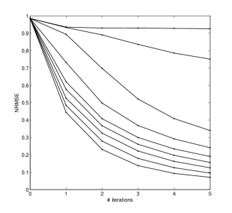
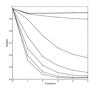
(a) (b)
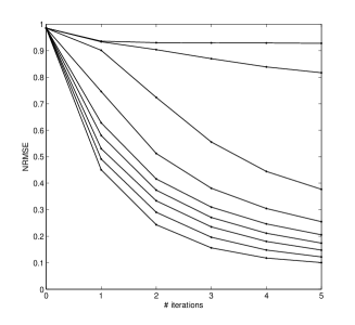
(c) (d)

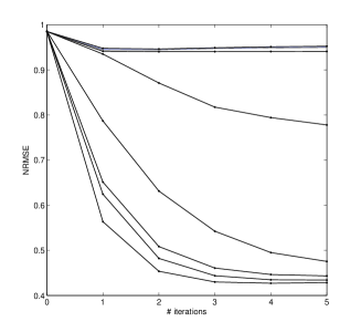
Figure 1: Prediction error evolvement of Bayesian spectral method for $N=100$, $D=30$, $M=10$. (a) linear matching, (b) thresholded ($f(x)=\tanh(x)$) match function ($\beta=1$)(c) noisy linear matching, , (d) noisy thresholded matching.

Using $N$, $D$, $M$ as free parameters, we randomly generated two matrices $\mathbf{X}$ and $\mathbf{W}$ with each components to be either 1 or -1. The match matrix $\mathbf{Y}$ was then computed as in section 2. We then investigated the capabilities of our algorithm in reconstructing the full matrix for 4 different cases: nearly perfect linear matching (little noise with $\sigma=0.01$ added), noisy linear matching ($\sigma=0.1$), nearly perfect thresholded match function ($f(x)=\tanh(x)$), and noisy thresholded matching.

Fixing $N=100$ and $D=30$, we applied the algorithm to two different data sets of $M=5$ and $M=10$. For each case, the unknown positions of the data matrix were randomly picked with missing percentages from 10% to 90%. For each missing percentage, an average result from 1000 runs were then obtained. The accuracy of predictions was measured by the popular used normalised root mean square error (NRMSE) after each iteration.

Figure 1 shows the evolvement of the algorithm prediction error through the first 5 iterations. The error at iteration 0 was calculated by replacing each missing position by the mean value of its corresponding subject. The 9 lines correspond to 9 different missing percentages, ranging from 10% to 90%. It can be seen that the algorithm converge quickly to reasonable accuracy after 5 iterations for up to 40% missing percentages in all cases. With too much missing data (80% upward for perfect linear data), the matrix could not be reconstructed. This phase transition corresponds to a rigidity percolation threshold. The noise moves this threshold down to 60%, but under perfect data collection condition, the nonlinear match function ($f(x)=\tanh(x)$) does not make any considerable effect. It comes to action however in the case of noisy data, moving the percolation threshold to 50%. In the case of linear matching data with very little noise, the rigid percolation threshold actually agrees with the theoretical result in  [5], which equals to $p=1-2M/N\simeq 80\%$

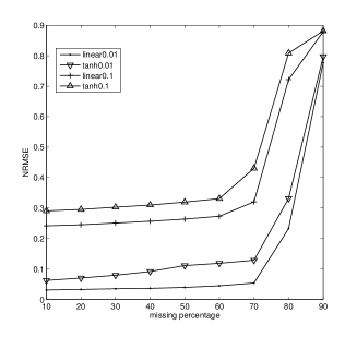
(a) (b)

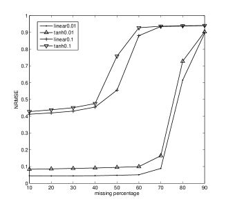
Figure 2: Prediction errors of Bayesian spectral method for the 4 reference cases. (a)$M=5$, (b)$M=10$

Figure 2 presents the effect of noise and nonlinearity on prediction accuracy. It could be easily seen the dramatic increase of error at the corresponding percolation thresholds. Noise shows critical effect on prediction accuracy compared to the thresholded match function, increasing by the complexity of data (large $M$).

4.2 Real data

To get a reasonable view of the phase transition, we applied the Bayesian spectral method on two different data sets. The first one is the measurements of the transcription levels under different experimental conditions of 215 mutants of essential yeast genes [18]. The dataset was extracted by the authors from microarray measurements of about 5000 genes of the budding yeast S.cerevisiae. The second dataset is the small-scale measurements of binding energies between the bacteria E.coli ligands and enzymes of the bacteria E.coli [20]. We removed all columns with missing values from the data, leaving two complete data matrices of size $215\times 15$ and $119\times 15$.

Following similar procedure to synthetic data tests, we randomly generated a list of missing positions in the complete data matrix, and cleared the known values out of those cells. We then applied the Bayesian spectral method to reconstruct the missing values on each data set, and compared to the original ones to calculate the prediction error. The procedure was applied for various missing percentage from 5% to 90%, for each case the average result from 1000 runs was obtained.

(a) (b)

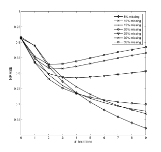
Figure 3: Missing value reconstruction of microarrays by the Bayesian spectral method. (a)prediction error for increasing missing percentage, (b)error evolvement of microarray data

The prediction results over increasing missing percentages of the two datasets are shown in figure 3a. The algorithm performs considerably better on the enzyme-ligand data than microarray data. Setting a threshold at a value of the NRMSE of $0.7$, where there is a big jump for the microarray data, we see that the algorithm is able to reconstruct enzyme-ligand values up to 70% missing, while the transition occurs at 20% missing for the case of microarray. Since enzyme-ligand data set was acquired by focused biochemistry studies of each enzyme, its reliability is a lot higher compared to the high-thoughput technique used to obtain gene expressions [21]. Apart from the common inaccuracy due to background noises and diversity of samples, the limitation of the measuring technology largely reduces microarray data reliability.

Figure 3b shows the prediction evolvement though early iterations for microarray data. Agreeing with the final prediction results, the algorithm kept improving its prediction by iterations with up to 20% missing data, while not much information can be reconstructed for data with 25% upward missing. Interestingly, in this case the error diminishes during the first 2 iterations, but then increases again. A similar effect was observed [22] in reconstructing missing values in synthetic data by means of linear regression and multi-entry correlations. Using the simplest algorithm [6, 8], missing values $\tilde{y}_{ij}$ are reconstructed by using two-entry correlations: $\tilde{y}_{ij}\propto\sum_{k}C_{jk}y_{ki}$, where $C_{ij}$ is the Pearson correlation among entries of subjects $i$ and $j$. For a large percentage of missing values, the correlation is affected by a low statistics, so one may try to exploit three- and higher-entry correlations. According with the level of noise, the number of hidden components and the nonlinearity of the matching function, this procedure improves the results only up to a certain point, after which the multi-entry contributions essentially furnish more noise than information, in a way similar to what is observed in Figure 3b. By looking at Figure 1, one can realize that in the case of noisy match (subfigures c and d), the evolvement curves of the error above the phase boundary (not converging phase) slightly rise after the first two iterations, while in the absence of noise (subfigures a and b) it keeps decreasing. This behavior suggests that in case of microarray, the level of noise is much greater that the level of nonlinearity.

5 Conclusions

We have applied a Bayesian spectral algorithm in order to investigate the nature of noise in synthetic and real datasets. The investigation on synthetic data shows that the approach is very robust in handling large percentage of missing data both in terms of accurate prediction and quick convergence rate. Although a solid conclusion on the ability of our method in predicting systems noise nature has not been made, the result on synthetic data and on some experimental datasets are very promising. A systematic investigation with specific consideration on different kinds of noises would prove useful.

References

References

- [1] The Netflix DVD rental store issued a 1 million prize for improving the accuracy of their predictions: http://www.netflixprize.com/
- [2] See for instance Amazon suggestions http://www.amazon.com/
- [3] See for instance Google searches http://www.google.com/
- [4] O. Troyanskaya, M. Cantor, G. Sherlock, P. Brown, T. Hastie, R. Tibshirani, D. Botstein and R. Altman (2001). Missing value estimation methods for DNA microarrays. Bioinformatics 17(6), 520–525.
- [5] S. Maslov and Y-C. Zhang (2001). Extracting Hidden Information from Knowledge Networks. Physical Review Letters 87(24), 248701_1–4.
- [6] F. Bagnoli, A. Berrones and F. Franci (2004). De gustibus disputandum (forecasting opinions by knowledge networks). Physica A 332, 509–518.
- [7] V.-A. Nguyen, Z. Nicola-Koulikova, F. Bagnoli, P. Lio’ (2008). Bayesian inference on hidden knowledge in high-throughput molecular biology data. To appear in LNAI PRICAI08 proceedings.
- [8] F. Bagnoli and F. Di Patti (2008). A biologically inspired classifier. Bio-Inspired Computing and Communication, P. Lió, J. Crowcroft, D. Verma, and E. Yoneki (eds), Lecture Notes in Computer Sciences 5150, Springer, pp. 320-327.
- [9] M.E. Tipping and C.M. Bishop (1999). Probabilistic principal component analysis. Journal of the Royal Statistical Society, Series B 61(3), 611–622.
- [10] Z. Koukolíková-Nicola, P. Liò, F. Bagnoli (2008). Inference on missing values in genetic networks using high-throughput data. Lecture Notes in Computer Science. 4973, Spriger, pp. 106–116.
- [11] R. Everson and S. Roberts (2000). Inferring the eigenvalues of covariance matrices from limited, noisy data. IEEE Trans Signal Processing 48, 2083–2091.
- [12] J.J. Rajan and P.J.W. Rayner (1997). Model order selection for the singular value decomposition and the discrete Karhunen-Loeve transform using a Bayesian approach. IEE Vison, Image and Signal Processing 144, 123–166.
- [13] T. Minka(2000). Automatic choice of dimensionality for PCA. Neural Information Processing Systems 13.
- [14] W.R. Gilks, B. Audit, D. de Angelis, S. Tsoka, C.A. Ouzounis (2005). Percolation of annotation errors through hierarchically structured protein sequence databases. Math BiosciFeb 193(2), 223–34.
- [15] W.R. Gilks, B. Audit, D. de Angelis, S. Tsoka, C.A. Ouzounis (2002). Modeling the percolation of annotation errors in a database of protein sequences. Bioinformatics 18(12), 1641–9.
- [16] A.O. Mooers, R.D.M. Page, A. Purvis and P.H. Harvey (1995). Phylogenetic Noise Leads to Unbalanced Cladistic Tree Reconstructions. Systematic Biology 44(3), 332–342
- [17] I. Comas, A. Moya and F. Gonzlez-Candelas (2007). Phylogenetic signal and functional categories in Proteobacteria genomes. BMC Evolutionary Biology 7(1):S7.
- [18] S. Mnaimneh, A.P. Davierwala, J. Haynes, J. Moffat, W. Peng, W. Zhang, X. Yang, J. Pootoolal, G. Chua, A. Lopez, M. Trochesset, D. Morse, N.J. Krogan, S.L. Hiley, Z. Li, Q. Morris, J. Grigull, N. Mitsakakis, C.J. Roberts, J.F. Greenblatt, C. Boone, C.A. Kaiser, B.J. Andrews, T.R. Hughes (2004). Exploration of Essential Gene Functions via Titratable Promoter Alleles. Cell 118(1), 31–44.
- [19] Smarkets is a Web-based, person-to-person betting exchange for Amazon Products http://www.midasoracle.org/2008/03/28/smarkets/
- [20] A. Macchiarulo, I. Nobeli and J. Thornton (2004). Ligand selectivity and competition between enzymes in silico. Nature Biotechnology 22(8), 1039–1045.
- [21] S. Draghicia, P. Khatria, A.C. Eklundb and Z. Szallasic (2006). Reliability and reproducibility issues in DNA microarray measurements. Trends in Genetics 22(2), 101–109.
- [22] F. Bagnoli, unpublished results.