Decoherence due to an excited state quantum phase transition in a two-level boson model

Abstract

The decoherence induced on a single qubit by its interaction with the environment is studied. The environment is modelled as a scalar two-level boson system that can go through either first order or continuous excited state quantum phase transitions, depending on the values of the control parameters. A mean field method based on the Tamm-Damkoff approximation is worked out in order to understand the observed behaviour of the decoherence. Only the continuous excited state phase transition produces a noticeable effect in the decoherence of the qubit. This is maximal when the system-environment coupling brings the environment to the critical point for the continuous phase transition. In this situation, the decoherence factor (or the fidelity) goes to zero with a finite size scaling power law.

I Introduction

Decoherence is the quantum phenomenon by which the coherence of a quantum system can be destroyed when it is put in contact with a large environment Zurek:03 ; Sch:04 . The Schröedinger equation is a linear differential equation, consequently any linear combination of solutions is also a solution of the problem. Thus, a general possible quantum state is a superposition of quantum states. Nevertheless, such a state does not appear in the classical macroscopic world. The decoherence interpretation of quantum mechanics Zurek:03 claims that this is due to the interaction with the environment, which destroys the quantum correlations between the states of the system, making it to transite from a quantum superposition state to a classical-like mixture of states. Moreover, only a small set of states take part of the classical-like mixture; they are called pointer states Zurek:03 .

The study of decoherence is important for several reasons: i) it might be responsible for the emergence of classical properties out of the underlying quantum nature of the physical systems, ii) it is a major problem for the construction of a quantum computer since it will produce the loss of the necessary quantum entanglement. Thus, both for fundamental reasons (i) and for practical purposes (ii) it is important to characterize the decoherence process and its effects on the physical properties of a quantum system.

Along this line of study, it is important to address the issue of the effect produced in the coherence of a quantum state when the environment evolves between different quantum phases. There have been several works on the relation between decoherence and an environmental quantum phase transition Paz:07 ; Paz:08 ; Rossini:07 ; Wang:08 ; Camalet:07 ; Yuan:07 . Recently, we have presented a novel phenomenon in which the decoherence of the system suffers drammatic changes when the environment crosses an excited state quantum phase transition (ESQPT)Relano:08 . An ESQPT is a nonanalytic evolution of the system as the control parameters in the Hamiltonian vary. It is similar to a ground state quantum phase transition but affecting to excited states. Correspondingly, an ESQPT can be classified in the thermodynamic limit as first order, when a crossing between two excited levels is present, or continuous, when the number of interacting levels is locally very large at an excited energy but without crossings.

In Ref. Relano:08 we presented briefly the case of a qubit in interaction with an environment modelled as a two-level boson system undergoing a continuous ESQPT. We used a particular simple Hamiltonian in terms of single control parameter to model the environment in order to show the main effect. Here we present a more extensive study of a similar system including both first and second order ESQPT, and more general sets of parameters. Together with the exact evolution of the system, we present a simple mean field treatment. We show that the decoherence is maximal when the interaction of the system with the environment produces second order ESQPT, while no noticeable effects are observed in the case of a first order ESQPT. For the former case, a finite-size scaling analysis allows us to postulate that the fidelity goes to zero as soon as the interaction between system and environment is switched on. We also show that mean field treatment provides a good description for the decoherence of the small system, except around the critical points.

The paper is structured as follows. In Sect. II, we present the model for the environment and study the phase diagram and its relation with the density of energy levels. We then discuss the interaction of the environment with the system. In Sect. III we show results for the decoherence factor. Both exact numerical results for large boson number, and an analytic mean field method with simple extensions of the Tamm-Dankoff approximation are presented. In Sect. IV, results for the decoherence factor in the case of continuous and first order ESQPT, including a finite size scaling study for the decoherence factor (or fidelity), are discussed. Finally, in Sect. V we summarize giving the main conclusions of this work.

II The Model

Following Paz:07 , we will consider our system composed by a spin $1/2$ particle coupled to a spin environment by the Hamiltonian $H_{\mathcal{SE}}$,

$$H_{\mathcal{SE}}=I_{\mathcal{S}}\otimes H_{\mathcal{E}}+\left|0\right>\left<0\right|\otimes H_{\lambda_{0}}+\left|1\right>\left<1\right|\otimes H_{\lambda_{1}},$$ (1)

where $\left|0\right>$ and $\left|1\right>$ are the two components of the spin $1/2$ system, and $\lambda_{0}$, $\lambda_{1}$ the couplings of each component to the environment. The three terms $H_{\mathcal{E}}$, $H_{\lambda_{0}}$ and $H_{\lambda_{1}}$ act on the Hilbert space of the environment; therefore, it evolves with an effective Hamiltonian depending on the state of the central spin $H_{i}=H_{\mathcal{E}}+H_{\lambda_{i}}$, $i=0,1$. The term $H_{\lambda_{i}}$ makes it possible that the environment crosses a critical point as a consequence of the interaction with the central spin Paz:07 .

Considering the initial state $\left|\Psi_{\mathcal{SE}}(0)\right>=(a\left|0\right>+b\left|1\right>)\left|\mathcal{E}(0)\right>$, where $\left|\mathcal{E}(0)\right>$ is the initial state of the environment, the evolved reduced density matrix of the system is

$$\rho_{\mathcal{S}}(t) = \mbox{Tr}_{\mathcal{E}}\left|\Psi_{\mathcal{SE}}(t)\right>\left<\Psi_{\mathcal{SE}}(t)\right|$$

$$= |a|^{2}\left|0\right>\left<0\right|+ab^{*}r(t)\left|0\right>\left<1\right|$$

$$+ a^{*}br^{*}(t)\left|1\right>\left<0\right|+|b|^{2}\left|1\right>\left<1\right|.$$

The off-diagonal terms of the density matrix are modulated by the decoherence factor $r(t)$ which is the overlap between two states of the environment obtained by evolving the initial state $\left|\Psi(0)\right>$ with two different Hamiltonians,

$$r(t)=\left<\Psi(0)\right|e^{iH_{0}t}e^{-iH_{1}t}\left|\Psi(0)\right>.$$ (3)

If the environment is initially in the ground state of $H_{0}$ , $\left|0,g\right>$, the decoherence factor, up to an irrelevant phase factor, is

$$r(t)=\left<0,g\right|e^{-iH_{1}t}\left|0,g\right>.$$ (4)

This quantity has the same form as the Loschmidt echo or the fidelity, and it contains all the relevant information about the decoherence process.

To be more specific, let us introduce as an environment a two-level boson system described by a generalized Lipkin Model, whose Hamiltonian is

$$H_{\mathcal{E}}=\alpha~{}\widehat{n}_{t}-\frac{1-\alpha}{N}~{}\widehat{Q}^{\omega}\widehat{Q}^{\omega},$$ (5)

where the operators $\widehat{n}_{t}$ and $\widehat{Q}^{\omega}$ are defined as

$$\widehat{n}_{t}=t^{{\dagger}}t,\hskip 14.22636pt\widehat{Q}^{\omega}=s^{{\dagger}}t+t^{{\dagger}}s+\omega~{}t^{{\dagger}}t,$$ (6)

in terms of two species of scalar bosons $s$ and $t$. $\alpha$ and $\omega$ are two independent control parameters, and the total number of bosons $N=\widehat{n}_{s}+\widehat{n}_{t}$ is a conserved quantity.

It is worth to mention that this two-level bosonic Hamiltonian is completely equivalent to an SU(2) spin Hamiltonian, with long-range spin exchange interaction. The equivalence is defined by the inverse Schwinger representation of the SU(2) generators

$$S^{+}=t^{\dagger}s=(S^{-})^{\dagger},\hskip 28.45274ptS^{z}=\frac{1}{2}(t^{\dagger}t-s^{\dagger}s),$$ (7)

where $S$ represents the total spin of a chain of $N$ 1/2 spins.

II.1 Mean field theory for $H_{\mathcal{E}}$

In order to study the phase diagram of the Hamiltonian (5) as a function of the control parameters $\alpha$ and $\omega$, it is usual to rely on a coherent state of the form

$$\left|N,\beta\right>=e^{\sqrt{\frac{N}{(1+\beta^{2})}}(s^{{\dagger}}+\beta~{}t^{{\dagger}})}\left|0\right>,$$ (8)

where $\left|0\right>$ denotes the boson vacuum. The corresponding energy surface as a function of the variational parameter $\beta$ is the expectation value of $H_{\mathcal{E}}$ (5) in the coherent state (8)

$$E(N,\beta) = \frac{\langle N,\beta|H_{\mathcal{E}}|N,\beta\rangle}{\langle N,\beta|N,\beta\rangle}$$ (9)

$$= N\frac{\beta^{2}}{(1+\beta^{2})^{2}}\Big{\{}5\alpha-4+4\beta\omega(\alpha-1)+\beta^{2}\big{[}\alpha+\omega^{2}(\alpha-1)\big{]}\Big{\}}.$$

Minimization of the energy (9) with respect to $\beta$, for given values of the control parameters $\alpha$ and $\omega$, gives the equilibrium value $\beta_{e}$ defining the phase of the system in the ground state. The value $\beta_{e}=0$ corresponds to the symmetric phase, and $\beta_{e}\not=0$ to the broken symmetry phase.

This Hamiltonian has a second order Quantum Phase Transition (QPT) along the line $\omega=0$, and a first order QPT for $\omega\not=0$. In the latter, the critical point is defined as the situation in which the minimum in the symmetric phase and in the broken symmetry phase are degenerate and their energies are equal to zero. The study of the phase diagram has been done in several publications Vidal:06 . Here we summarize its main features.

• $\beta=0$ is always a stationary point. For $\omega=0$, the solution with $\beta=0$ is a maximum for $\alpha<4/5$, and becomes a minimum for $\alpha>4/5$. In the case of $\alpha=4/5$, $\beta=0$ is an inflection point. $\alpha=4/5$ is the point in which a minimum at $\beta=0$ starts to develop and defines the antispinodal line.

• For $\omega\neq 0$ there exists a region where two minima, one spherical and one deformed, coexist. This region is defined by the point where the $\beta=0$ minimum appears (antispinodal point) and the point where the $\beta\neq 0$ minimum appears (spinodal point). The spinodal line is defined by the implicit equation,

  $$\frac{3\,\alpha}{3\,\alpha-4}=\frac{\cal A}{\cal B}\left(1-\left(1+\frac{\cal B}{\cal A}\right)^{\frac{3}{2}}\right),$$ (10)

  where ${\cal A}=(4-3\,\alpha+2\,(\alpha-1)\,\omega^{2})^{2}$ and ${\cal B}=36\,\omega^{2}\,(\alpha-1)^{2}$. For example, for $\omega=1/\sqrt{2}$, $\alpha\simeq 0.822559$.

• In the coexistence region, the critical point is defined by the condition that both minima (spherical and deformed) are degenerate. At the critical point the two degenerated minima are at $\beta_{e}=0$ and $\beta_{e}=\omega/2$, and their energy is equal to zero. The critical line is therefore defined as

  $$\alpha_{c}=\frac{4+\omega^{2}}{5+\omega^{2}}.$$ (11)

  For example, for $\omega=1/\sqrt{2}$, $\alpha_{c}=9/11$.

• According to the previous analysis, for $\omega\neq 0$ there appears a first-order phase transition, while for $\omega=0$ there is an isolated point of second-order phase transition at $\alpha=4/5$. In this case, antispinodal, spinodal and critical points collapse to a single point.

Figure 1: Schematic phase diagram for $H_{\mathcal{E}}$ (5) as a function of the control parameters $\alpha$ and $\omega$.

In Fig. 1 we present a schematic view of the phase diagram for the environment Hamiltonian $H_{\mathcal{E}}$ (5) in the $\omega-\alpha$ plane.

The Hamiltonian (5) also displays an Excited State Quantum Phase Transition (ESQPT), which is analogous to a standard quantum phase transition, but taking place at some excited critical energy $E_{c}$ of the system. We can distinguish between different kinds of ESQPTs. As it is stated in Cejnar:07 , in the thermodynamic limit a crossing of two levels at $E=E_{c}$ determines a first order ESQPT, while if the number of interacting levels is locally large at $E=E_{c}$ but without real crossings, the ESQPT is continuous. As the entropy of a quantum system is related to its density of states, a relationship between an ESQPT and a standard phase transition at a certain critical temperature can be established in the thermodynamic limit Cejnar:09 . These kinds of phase transitions have been identified in the Lipkin model Heiss:05 , in the interacting boson model Heinze:06 , and in more general boson or fermion two-level pairing Hamiltonians (for a complete discussion, including a semiclassical analysis, see Caprio:08 ). In all these cases, the ESQPT takes place beyond the critical value of the Hamiltonian control parameter, implying that the critical point moves from the ground state to an excited state.

(a) $\omega=0$	(b) $\omega=1/\sqrt{2}$

Figure 2: Energy levels of the Hamiltonian (5) as a function of $\alpha$ for $N=50$ and two different values of $\omega$.

In Fig. 2 we show the energy eigenvalues of the environmental Hamiltonian (5) with $N=50$ bosons as a function of the control parameter $\alpha$ for $\omega=0$ in left panel, and $\omega=1/\sqrt{2}$ in right panel. In both cases, we see for $\alpha<\alpha_{c}$ a collapse of several levels at $E\approx 0$. In the right panel ($\omega=1/\sqrt{2}$) we can also see a second critical curve for $E<0$ that divides the level diagram in two regions: one in which levels behave smoothly, and another in which the level density increases and some crossings are observed.

One simple way to analyze the phase diagram is by means of the density of states. To obtain an analytical approximation for this quantity, one can start from a coherent state similar to (8), in which real parameter $\beta$ is replaced by the complex parameter $z=\tan\left(\phi/2\right)\exp\left(i\xi\right)$, in terms of which the energy is expressed as $\mathcal{H}(\phi,\xi)=\left<N,\phi,\xi\right|H\left|N,\phi,\xi\right>$. A good approximation for the density of states can be obtained by counting how many levels are there in an energy window $dE$,

$$\rho(E)=\frac{1}{\mathcal{N}}\int d\xi d\phi\left|J(\phi,\xi)\right|\delta\left(\mathcal{H}(\phi,\xi)-E\right),$$ (12)

where $\left|J(\phi,\xi)\right|$ is the Jacobian of the transformation $\left(\phi,\xi\right)\rightarrow(p,q)$, $p$ and $q$ are the canonical coordinates of the Hamiltonian, and $\mathcal{N}$ is a normalization constant.

Figure 3: Density of states of the Hamiltonian (5) for $N=1000$, $\alpha=0.5$. The dashed line corresponds to $\omega=0$ and the dotted line to $\omega=1/\sqrt{2}$.

In Fig. 3 we show the density of levels of the environmental Hamiltonian (5), calculated by means of Eq. (12), for $N=1000$, $\alpha=1/2$ and the same values of $\omega$ as in Fig. 2. As it can be seen, the collapse of levels at $E=0$ gives rise to a cusp singularity of $\rho(E)$ for both $\omega=0$ and $\omega=1/\sqrt{2}$. In the latter case, there also exists a jump in the density of states for a fixed value $E<0$ ($E\approx-125$ for this value of $\omega$) consistent with the energy spectra of Fig. 2. Although not shown, similar results are obtained for other values of $\alpha$ and $\omega$. In particular, the jump in the density of states at a certain value $E<0$ only appears for $\omega>0$. Therefore, two different kinds of ESQPT exist in excited spectrum of Hamiltonian (5). If we keep the terminology of thermodynamical phase transitions and we take the number of levels up to an energy E, $N(E)=\int dE\rho(E)$ as the analogue of the free energy $F(N,T)$, we can conclude: (a) there exists a continuous $\lambda$ quantum phase transition at $E^{(2)}_{c}=0$, for any value of parameter $\omega$; (b) there also exists a first-order quantum phase transition at some critical energy $E^{(1)}_{c}<0$ if $\omega>0$.

To estimate the critical energies at which these quantum phase transitions take place, we can rely on the energy surface $\mathcal{H}(\phi,\xi)$. In Fig. 4 we show $\mathcal{H}(\phi,\xi)/N$ in the thermodynamical limit $N\rightarrow\infty$ for $\alpha=1/2$ and $\omega=1/\sqrt{2}$. The curves drawn in the base of the figure are contour curves for fixed values of the energy $\mathcal{H}(\phi,\xi)/N=E$. Gray curves (red online) represent different values of $E$ around $E^{(2)}_{c}$ for the continuous phase transition. The solid gray (red online) line represents the critical point $E_{c}=0$; this is the only value for which the contour curve is non-analytic. On the other hand, black curves (blue online) represent different values of $E$ around the critical energy at which the first-order ESQPT takes place, $E^{(1)}_{c}$. In this case, the critical value is the one at which the island around $\xi=\pi$ appears, that correspond to a local minimum in the energy surface. This entails the appearance of another region in the $(\phi,\xi)$ plane for which the equation $\mathcal{H}(\phi,\xi)/N=E$ has a solution, and consequently the density of states $\rho(E)$ suddenly increases.

Figure 4: (Color online). Energy surface $\mathcal{H}(\phi,\xi)/N$ in the thermodynamical limit $N\rightarrow\infty$ for $\alpha=1/2$ and $\omega=1/\sqrt{2}$. Contour curves are drawn on the base of the figure (see text).

II.2 Coupling to a single qubit

Since we are interested in relating the phenomenon of decoherence in a single qubit with the structure of phases and critical regions in the environment as defined by the Hamiltonian (1), we propose as a coupling Hamiltonian $H_{\lambda_{i}}=\lambda_{i}\widehat{n_{t}}$. Choosing $\lambda_{0}=0$ if the qubit is on state $\left|0\right>$ and $\lambda_{1}=\lambda$ if the qubit is on the state $\left|1\right>$, the effective environment Hamiltonian for each component of the system results into

$$H_{0} = \alpha~{}\widehat{n}_{t}-\frac{1-\alpha}{N}~{}\widehat{Q}_{t}\widehat{Q}_{t},$$ (13)

$$H_{1} = (\alpha+\lambda)\widehat{n}_{t}-\frac{1-\alpha}{N}~{}\widehat{Q}_{t}\widehat{Q}_{t}~{}.$$ (14)

This means that the qubit only interacts with the environment when it is on state $\left|1\right>$.

The system-environment coupling parameter $\lambda$ modifies the environment Hamiltonian. For certain values of $\alpha$ and $\lambda$, this modification entails a crossing of the critical lines. Similar phenomena were previously analyzed by several authors Paz:07 ; Paz:08 ; Rossini:07 , studying whether a quantum quench that drives the environment through a QPT implies some kind of universality in the decoherence process.

Using the coherent state approach Vidal:06 , it is straightforward to show that $H_{1}$ goes through a ground state QPT at

$$\lambda_{*}=(1-\alpha)(4+\omega^{2})-\alpha$$ (15)

for $\alpha<\alpha_{*}$. Therefore, if $\lambda>\lambda_{*}$ the quench makes the environment jump from one phase to the other.

The main purpose of this paper to show that an ESQPT, instead of a ground state QPT, indeed produces dramatic consequences in the decoherence process. Using the coherent state approximation, it is straightforward to obtain that the coupling between the environment and the qubit entails an energy transfer in the former one, which is equal to

$$\Delta E(N,\beta,\lambda)=\left<N,\beta\right|\lambda\widehat{n_{t}}\left|N,\beta\right>=\lambda N\frac{\beta^{2}}{1+\beta^{2}}.$$ (16)

Therefore, the critical coupling $\lambda_{c}$ which leads the environment to the critical energy $E_{c}$ is

$$E(N,\beta)+\Delta E(N,\beta,\lambda_{c})=E_{c},$$ (17)

valid for both first order critical energy $E_{c}^{(1)}$ and second order one $E_{c}^{(2)}$. In general, this is a trascendent equation, and therefore $\lambda^{(1)}_{c}$ and $\lambda^{(2)}_{c}$ (the $\lambda$’s corresponding to $E_{c}^{(1)}$ and $E_{c}^{(2)}$, respectively) have to be obtained numerically.

III Calculation of the decoherence factor

In order to calculate the decoherence factor (4) the expectation value of $H_{1}$ (14) in the ground state $|0,g\rangle$ of $H_{0}$ (13) is needed. The decoupling of the complete system-environment Hamiltonian into the independent Hamiltonians $H_{0}$ and $H_{1}$ for each qubit state allows an exact diagonalization for large systems. In the following two subsections we will describe the exact formalism and make a comparison with mean field techniques supplemented with a Tamm-Dankoff approximation (TDA) treatment of the excited spectrum.

III.1 Exact diagonalization

A general Hamiltonian in terms of $s$ and $t$ bosons including up to two body terms is,

$$H_{st} = at^{\dagger}t+b(t^{\dagger}s+s^{\dagger}t)+ct^{\dagger}ss^{\dagger}t$$ (18)

$$+ d(t^{\dagger}st^{\dagger}s+s^{\dagger}ts^{\dagger}t)+e(t^{\dagger}st^{\dagger}t+t^{\dagger}ts^{\dagger}t)+ft^{\dagger}tt^{\dagger}t$$

where $a,b,c,d,e$ and $f$ are arbitrary parameters.

Both Hamiltonians, $H_{0}$ (13) and $H_{1}$ (14), are particular cases of $H_{st}$ (18) with the following parameters,

$$a = \alpha+\lambda-2\frac{\alpha-1}{N}$$

$$b = \omega\frac{\alpha-1}{N}$$

$$c = 2\frac{\alpha-1}{N}$$

$$d = \frac{\alpha-1}{N}$$

$$e = 2\omega\frac{\alpha-1}{N}$$

$$f = \omega^{2}\frac{\alpha-1}{N}$$

$$\Delta = \alpha-1,$$ (19)

where $\Delta$ is an irrelevant global shift in energy.

The exact diagonalization of the $st$ Hamiltonian (18), and consequently of $H_{0}$ and $H_{1}$, reduces to the diagonalization of a tridiagonal matrix in the basis

$$|Nl\rangle=\frac{{t^{\dagger}}^{l}{s^{\dagger}}^{N-l}}{\sqrt{l!(N-l)!}}|0\rangle,$$ (20)

where $|0\rangle$ is the boson vacuum and $0\leq l\leq N$. Therefore, the dimension of the Hamiltonian matrix is $d=N+1$.

The relevant matrix elements are,

$$\langle Nl|H_{st}|Nl\rangle = al+fl^{2}+cl(1+N-l),$$ (21)

$$\langle Nl|H_{st}|Nl+1\rangle = b\sqrt{(N-l)(l+1)}+e\sqrt{(l+1)(N-l)}~{}l,$$ (22)

$$\langle Nl|H_{st}|Nl+2\rangle = d\sqrt{(l+2)(l+1)}\sqrt{(N-l)(N-l-1)},$$ (23)

being all the others equal to zero. The diagonalization of the corresponding tridiagonal matrix can be done easily even for large $N$ values, providing the exact results for the eigenenergies and eigenfunctions of $H_{0}$ and $H_{1}$ and consequently allowing to calculate numerically $r(t)$.

III.2 The Tamm-Dankoff approximation

Before applying the exact diagonalization techniques to study the behavior of the decoherence as a fuction of the set of model parameters and particularly in relation to the quantum phase transitions (first and second order) in the ground (QPT) and excited states (ESQPT) of the environment, we will introduce an extension of the mean field approximation based on the TDA but including two phonon anharmonicities.

Let us consider the condensate boson of the state (8) as a ground state deformed boson in a rotated basis. Since two Hamiltonians are involved, $H_{0}$ and $H_{1}$, let us formulate the approximation for both in terms of a generic $H_{i}$ ($i=0,1$). The variational parameter $\beta$ in the condensate could be different for both Hamiltonians; therefore, the notation $\beta_{i}$ ($i=0,1$) will be used to distinguish between both cases. With this notation, the deformed bosons ($g$ and $e$) for $H_{i}$ are related to the initial ones ($s$ and $t$ bosons) by

$$\Gamma^{{\dagger}}_{i,g} = \frac{1}{\sqrt{1+\beta_{i}^{2}}}(s^{{\dagger}}+\beta_{i}t^{{\dagger}}),$$ (24)

$$\Gamma^{{\dagger}}_{i,e} = \frac{1}{\sqrt{1+\beta_{i}^{2}}}(-\beta_{i}s^{{\dagger}}+t^{{\dagger}}).$$ (25)

In terms of the deformed bosons the ground state and the first excited states are

$$\left|i,g\right> = \frac{1}{\sqrt{N!}}\left(\Gamma_{i,g}^{{\dagger}}\right)^{N}\left|0\right>,$$ (26)

$$\left|i,e\right> = \frac{1}{\sqrt{(N-1)!}}\Gamma_{i,e}^{{\dagger}}(\Gamma_{i,g}^{{\dagger}})^{N-1}\left|0\right>.$$ (27)

In this framework, higher excited states can be constructed by directly replacing a ground state boson condensate by an excited $\beta$ boson; this procedure is known as the Tamm-Dancoff approximation (TDA) method. In addition, with this basis is possible to write a diagonal Hamiltonian in terms of the new bosons. If only one body terms are included,

$$H_{i} \approx \left<i,g|H_{i}|i,g\right>+\Big{(}\left<i,e|H_{i}|i,e\right>-\left<i,g|H_{i}|i,g\right>\Big{)}\Gamma^{{\dagger}}_{i,e}\Gamma_{i,e}$$

$$=E_{i,0}+\Delta_{e_{i}}\Gamma^{{\dagger}}_{i,e}\Gamma_{i,e},$$

where $E_{i,0}=\left<i,g|H_{i}|i,g\right>$ and $\Delta_{e_{i}}=\left(\left<i,e|H_{i}|i,e\right>-\left<i,g|H_{i}|i,g\right>\right)$.

The calculation for $r(t)$ (4) involves the $H_{0}$ ground state and the Hamiltonian $H_{1}$. Thus, it is necessary to relate the intrinsic bosons for $H_{0}$ and $H_{1}$. The relation between both boson families is given by

$$\Gamma^{{\dagger}}_{0,g} = \sum_{p}~{}f_{gp}~{}\Gamma_{1,p}^{{\dagger}},$$ (29)

$$\Gamma^{{\dagger}}_{0,e} = \sum_{p}~{}f_{\beta p}~{}\Gamma_{1,p}^{{\dagger}},$$ (30)

where this sum is for $p=g$ and $p=e$, and the coefficients of the needed transformation are,

$$f_{gg} = \frac{1}{\sqrt{1+\beta_{0}^{2}}}\frac{1}{\sqrt{1+\beta_{1}^{2}}}(1+\beta_{0}\beta_{1}),$$ (31)

$$f_{ge} = \frac{1}{\sqrt{1+\beta_{0}^{2}}}\frac{1}{\sqrt{1+\beta_{1}^{2}}}(\beta_{0}-\beta_{1}).$$ (32)

With the preceding transformation it is possible to write $\left|0,g\right>$ in terms of the $H_{1}$ intrinsic bosons

$$\left|0,g\right>=\frac{1}{\sqrt{N!}}\left(f_{gg}\Gamma_{1,g}^{{\dagger}}+f_{ge}\Gamma_{1,e}^{{\dagger}}\right)^{N}\left|0\right>.$$ (33)

Using the binomial expansion of (33) is then straightforward to calculate the decoherence factor $r(t)$ using the TDA basis up to an irrelevant phase factor

$$r(t)=\sum_{k=0}^{N}\binom{N}{k}~{}\left(f_{gg}\right)^{2(N-k)}~{}\left(f_{ge}\right)^{2k}~{}e^{-i\Delta_{e_{1}}kt},$$ (34)

where $\Delta_{e_{1}}=\left(\left<1,e|H_{1}|1,e\right>-\left<1,g|H_{1}|1,g\right>\right)$. A more compact expression for $r(t)$ can be obtained using the transformation,

$$e^{-i\Delta_{e_{1}}tk}=e^{-i(\Delta_{e_{1}}/2)tN}~{}e^{i(\Delta_{e_{1}}/2)t(N-k)}~{}e^{-i(\Delta_{e_{1}}/2)tk}.$$ (35)

Therefore, the decoherence factor $r(t)$ in the TDA reduces to

$$r(t)=e^{-i(\Delta_{e_{1}}/2)tN}\left(\left(f_{gg}\right)^{2}~{}e^{i(\Delta_{e_{1}}/2)t}+\left(f_{ge}\right)^{2}~{}e^{-i(\Delta_{e_{1}}/2)t}\right)^{N}.$$ (36)

The matrix elements required for calculating $r(t)$ are

$$\langle i,g|H_{i}|i,g\rangle = (a+c+f)\frac{\beta_{i}^{2}}{1+\beta_{i}^{2}}N+2b\frac{\beta_{i}}{1+\beta_{i}^{2}}N$$ (37)

$$+ \frac{N(N-1)}{(1+\beta_{i}^{2})^{2}}\Big{(}(c+2d)\beta_{i}^{2}+2e\beta_{i}^{3}+f\beta_{i}^{4}\Big{)},$$

and

$$\langle i,e|H_{i}|i,e\rangle = \frac{1}{1+\beta_{i}^{2}}(a+c+f-2b\beta_{i})+c\frac{(1-\beta_{i}^{2})^{2}}{(1+\beta_{i}^{2})^{2}}(N-1)$$ (38)

$$+ \frac{4(N-1)}{(1+\beta_{i}^{2})^{2}}(f\beta_{i}^{2}-2d\beta_{i}^{2}+e(\beta_{i}-\beta_{i}^{3}))$$

$$+ (a+c+f)\frac{\beta_{i}^{2}}{1+\beta_{i}^{2}}(N-1)+2b\frac{\beta_{i}}{1+\beta_{i}^{2}}(N-1)$$

$$+ \frac{(N-1)(N-2)}{(1+\beta_{i}^{2})^{2}}\Big{(}(c+2d)\beta_{i}^{2}+2e\beta_{i}^{3}+f\beta_{i}^{4}\Big{)}.$$

A simple inspection reveals that decoherence factor $r(t)$ (36) does not give a good approximation of the exact results (see below and Relano:08 ). The modulus of $r(t)$ is

$$\left|r(t)\right|=\left|\left(f_{gg}^{2}\right)e^{i\left(\Delta_{e_{1}}/2\right)t}+\left(f_{ge}^{2}\right)e^{-i\left(\Delta_{e_{1}}/2\right)t}\right|^{N}=\left|f_{ge}\right|^{2N}\left|\left(\frac{f_{gg}}{f_{ge}}\right)^{2}+e^{i\Delta_{e_{1}}t}\right|^{N}.$$ (39)

As a particular example, let us consider $\beta_{1}=0$ and $\beta_{0}\neq 0$, that is, the situation in which the coupling of the qubit to the environment forces the environments to cross the phase transition from the broken phase to the symmetric phase. In this situation

$$f_{gg} = \frac{1}{\sqrt{1+\beta_{0}^{2}}}$$ (40)

$$f_{ge} = \frac{\beta_{0}}{\sqrt{1+\beta_{0}^{2}}}.$$ (41)

From these expressions, it is straightforward to obtain that $\left|r(t)\right|$ oscillates between

$$\left|r(t)\right|_{\text{max}} = 1;$$ (42)

$$\left|r(t)\right|_{\text{min}} = \left|\frac{\beta_{0}^{2}-1}{\beta_{0}^{2}+1}\right|^{N}\longrightarrow 0,\;\text{for}\;N\longrightarrow\infty.$$ (43)

Therefore, we can conclude that TDA approximation including just one phonon excitations does not account for the decay of the envelope of the decoherence factor reported in Relano:08 (see below for more details). This evidence suggests to go further within the spirit of TDA by including the anharmonicities of the two-phonon excitations. For this purpose it is needed to construct the states two TDA excitations as

$$\left|i,e^{2}\right> = \frac{1}{\sqrt{2}}\frac{1}{\sqrt{(N-2)!}}(\Gamma_{i,e}^{{\dagger}})^{2}(\Gamma_{i,g}^{{\dagger}})^{N-2}\left|0\right>.$$ (44)

From this state we derive the diagonal part of the Hamiltonian as

$$\begin{split}H_{i}&\approx\langle i,g|H_{i}|i,g\rangle+\Big{(}\langle i,e|H_{i}|i,e\rangle-\langle i,g|H_{i}|i,g\rangle\Big{)}\Gamma^{{\dagger}}_{i,e}\Gamma_{i,e}\\ &+\left(\frac{\langle i,e^{2}|H_{i}|i,e^{2}\rangle}{2}-\langle i,e|H_{i}|i,e\rangle+\frac{\langle i,g|H_{i}|i,g\rangle}{2}\right)\Gamma^{{\dagger}}_{i,e}\Gamma^{{\dagger}}_{i,e}\Gamma_{i,e}\Gamma_{i,e}\\ &=E_{i,0}+\Delta_{e_{i}}\Gamma^{{\dagger}}_{i,e}\Gamma_{i,e}+\Omega_{e_{i}}\Gamma^{{\dagger}}_{i,e}\Gamma^{{\dagger}}_{i,e}\Gamma_{i,e}\Gamma_{i,e},\end{split}$$ (45)

where $E_{i,0}=\langle i,g|H_{i}|i,g\rangle$, $\Delta_{e_{i}}=\left(\langle i,e|H_{i}|i,e\rangle-\langle i,g|H_{i}|i,g\rangle\right)$, and $\Omega_{e_{i}}=\left(\frac{\langle i,e^{2}|H_{i}|i,e^{2}\rangle}{2}-\langle i,e|H_{i}|i,e\rangle+\frac{\langle i,g|H_{i}|i,g\rangle}{2}\right)$.

With the preceding transformation (33) we can obtain the decoherence factor in the improved approximation up to an irrelevant phase factor

$$r(t)=\sum_{k=0}^{N}\binom{N}{k}~{}\left(f_{gg}\right)^{2(N-k)}~{}\left(f_{ge}\right)^{2k}~{}e^{-i(\Delta_{e_{1}}k+\Omega_{e_{1}}k(k-1))t}.$$ (46)

In addition to (37) and (38), the only needed matrix element for obtaining $r(t)$ is $\Omega_{e_{1}}$ which follows from $\langle i,g|H_{i}|i,g\rangle$, $\langle i,e|H_{i}|i,e\rangle$, given above and

$$\langle i,e^{2}|H_{i}|i,e^{2}\rangle = \frac{1}{(1+\beta_{i}^{2})^{2}}\Big{(}(2c+4d)\beta^{2}_{i}+4e\beta_{i}^{3}+2f\beta_{i}^{4}\Big{)}$$ (47)

$$+ \frac{2}{1+\beta_{i}^{2}}(a+c+f-2b\beta_{i})+2c\frac{(1-\beta_{i}^{2})^{2}}{(1+\beta_{i}^{2})^{2}}(N-2)$$

$$+ \frac{8(N-2)}{(1+\beta_{i}^{2})^{2}}(f\beta_{i}^{2}-2d\beta_{i}^{2}+e(\beta_{i}-\beta_{i}^{3}))$$

$$+ (a+c+f)\frac{\beta_{i}^{2}}{1+\beta_{i}^{2}}(N-2)+2b\frac{\beta_{i}}{1+\beta_{i}^{2}}(N-2)$$

$$+ \frac{(N-2)(N-3)}{(1+\beta_{i}^{2})^{2}}\Big{(}(c+2d)\beta_{i}^{2}+2e\beta_{i}^{3}+f\beta_{i}^{4}\Big{)}.$$

Inserting (37), (38) and (47) into (46) we arrive to the final form of the decoherence factor $r(t)$ within the extended TDA approximation. In this case, a semi-quantitative analysis as the previous one cannot be easily done. A comparison with exact numerical calculations is performed in next section.

IV Results

In this section we present the main features of evolution of the system described by (1) under the influence of the environment given by (5). A brief report of the relationship between the decoherence in the qubit and the excited state quantum phase transitions in the environment was given in Relano:08 . Here, we extend the analysis, comparing the numerical results with the Tamm-Dankoff approximation, and also facing the case of $\omega\neq 0$, that was not considered in Relano:08 . As two paradigmatic cases, we deal with the cases $\alpha=1/2$, and $\omega=0$ and $\omega=1/\sqrt{2}$. Different choices for the defining parameters of the model give rise to the same qualitative results.

IV.1 Decoherence factor for the Continuous ESQPT

All the information about the decoherence process induced by the environment (5) in the central qubit is encoded in the decoherence factor (4). As mentioned above, for the Hamiltonian we are using there is always a continuous ESQPT independently of the value of $\omega$. In addition, for $\omega\neq 0$ there also appears a first order ESQPT. In this subsection we will analyze the effect of the continuous ESQPT on the decoherence factor, while the effect of the first order ESQPT on the decoherence factor will be discussed in the next subsection.

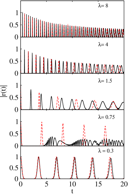
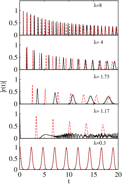
(a) $\omega=0$	(b) $\omega=1/\sqrt{2}$

Figure 5: (Color online) $|r(t)|$ for $\alpha=1/2$ and five different values of $\lambda$ for two selections of the coupling system-environment parameter $\omega$, $\omega=0$ on the left and $\omega=1/\sqrt{2}$ on the right. In all cases $N=1000$. Solid (black) lines correspond to the exact solution, and dashed (red) lines to the TDA calculation.

In Fig. 5 we show the results for the decoherence factor for $N=1000$ bosons and $\alpha=1/2$, for two $\omega$ values, $\omega=0$ (left panels) and $\omega=1/\sqrt{2}$ (rigth panels). The objective of this figure is to show the effect of the continuous ESQPT on the decoherence factor. Solving Eq. (17) for the value of $\alpha=1/2$, the continuous ESQPT ($E_{c}^{(2)}=0$) takes place at $\lambda_{c}^{(2)}=0.75$ for $\omega=0$ (left panel) and at $\lambda_{c}^{(2)}=1.17$ for $\omega=1/\sqrt{2}$ (right panel). Several features deserve to be discussed. First of all, we can see that the TDA calculation works pretty well for small and large values of $\lambda$. In particular, the shape of the envelope, which remains unaffected by the increase of $\lambda$ for $\lambda\gg\lambda_{c}^{(2)}$, is very well described by the TDA calculation (see panels for $\lambda=4$ and $\lambda=8$ in Fig. 5). Since this approximation mainly relies on the position of the first and the second excited states of $H_{\mathcal{E}}$, we can conclude that the information contained in the low energy spectrum is enough to have a good idea about the properties of the highest excited levels of the environmental Hamiltonian. Note that switching on the interaction between the central qubit and the environment entails an effective increase of the environmental energy roughly given by $\Delta E=\left<g_{0}\right|H_{1}(\lambda)\left|g_{0}\right>-E_{0}$, and therefore a large value of $\lambda$ implies that the state of the environment jumps from the ground state to a mixed high-energy state.

On the other hand, as it is clearly shown in the left panels corresponding to $\lambda=\lambda_{c}^{(2)}=0.75$ and $\lambda=\lambda_{*}=1.5$, and the right panels $\lambda=\lambda_{c}^{(2)}=1.17$ and $\lambda=\lambda_{*}=1.75$, the TDA calculations fails for intermediate values of $\lambda$. These two values correspond to the critical couplings $\lambda_{c}^{(2)}$ and $\lambda_{*}$, corresponding to the excited state and the ground state quantum phase transitions, given by Eqs. (17) and (15) respectively. The reason why the Tamm-Dankoff approximation does not work for these values is straightforward. The ESQPT entails a singularity in the energy spectrum far above the first excited state, which gives rise to the main contribution in the TDA calculation. On the other hand, the ground state QPT does not affect the decoherence suffered by the central qubit because the coupling $\lambda$ makes the environment to jump far above the critical point which entails a singularity in the gap between the ground and the first excited states. However, as the TDA calculation for $r(t)$ strongly depends on this gap, it is spuriously affected by the QPT induced by the critical coupling $\lambda_{*}$.

Finally, the best agreement between the Tamm-Dankoff approximation and the exact calculation happens for $\lambda=0.3$, far below $\lambda_{c}^{(2)}$. Not only the envelope of the decoherence factor is well reproduced, but also the positions of the local maximum are well placed. In this case, the small coupling makes the environment to jump from the ground state to a mixed low-energy state. Therefore, it is reasonable to assume that the description provided by the TDA, which only takes in consideration the first excited state and a global measure of the anharmonicites of the spectrum, is a better approximation for small values of $\lambda$.

IV.1.1 Analysis of the critical behavior of the decoherence at the continuous ESQPT

As it is shown in Fig. 5, the decoherence of the central qubit behaves in a singular way for a critical coupling $\lambda_{c}^{(2)}$, which makes the environment to jump to the critical energy $E^{(2)}_{c}=0$. As the density of states in both cases $\omega=0$ and $\omega\neq 0$ display the same critical behavior around this value (see Fig. 3), also the same singular behavior for the decoherence is expected.

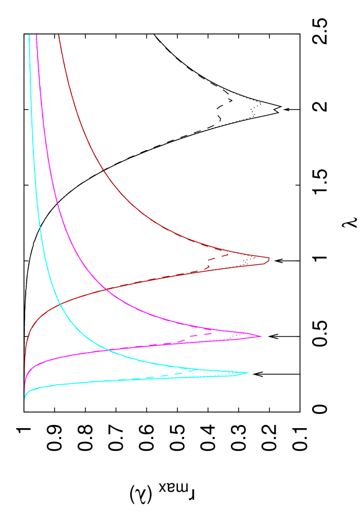
(a) $\omega=0$	(b) $\alpha=1/2$

Figure 6: (Color online) $r_{max}$ in function of the coupling $\lambda$, for different values of $\alpha$, $\omega$, and N. In left panel $\omega=0$. Black lines represent the case $\alpha=0$; dark gray (red online) lines, $\alpha=0.4$; gray (magenta online), $\alpha=0.6$; and light gray (cyan online), $\alpha=0.7$. Solid lines represent N =10 000; dotted lines, N=2500; and dashed lines, N=600. In right panel, $\alpha=1/2$, and lines represent the cases $\omega=0.2$, $\omega=1/2$, $\omega=1/\sqrt{2}$, and $\omega=1$, with the same color code than right panel. Arrows show the critical coupling $\lambda_{c}$ provided by Eq. (17).

In. Fig. 6 we show $r_{max}(\lambda)$, defined as the second maximum of $|r(t)|$ (the first maximum is trivially $|r(t=0)|=1$). The left panel displays the case $\omega=0$ for several values of $\alpha$, and the right panel the case $\alpha=1/2$, for several values of $\omega\neq 0$ (see caption for details). We can see that the behavior of this quantity is the same for $\omega=0$ and $\omega\neq 0$. It evolves smoothly and independently of the size of the system $N$ for values far from the critical coupling $\lambda_{c}^{(2)}$, provided by Eq. (17) and shown in Tab. 1. In a small region around $\lambda\sim\lambda_{c}^{(2)}$, $r_{max}$ becomes sharp, and the value of the minimum depends on the size of the system $N$; the larger is the system, the smaller is $r_{max}(\lambda_{c}^{(2)})$. Therefore, for both $\omega=0$ and $\omega\neq 0$, the decoherence factor behaves in a critical way around $\lambda=\lambda_{c}^{(2)}$ where $r_{max}(\lambda_{c}^{(2)})$ undergoes a dip towards zero which is sharper and deeper for larger values of N.

$\omega=0$				$\alpha=1/2$
$\alpha=0$	$\alpha=0.4$	$\alpha=0.6$	$\alpha=0.7$	$\omega=0.2$	$\omega=0.5$	$\omega=1/\sqrt{2}$	$\omega=1$
$\lambda_{c}^{(2)}=2$	$\lambda_{c}^{(2)}=1$	$\lambda_{c}^{(2)}=0.5$	$\lambda_{c}^{(2)}=0.25$	$\lambda_{c}^{(2)}=0.83$	$\lambda_{c}^{(2)}=1.01$	$\lambda_{c}^{(2)}=1.17$	$\lambda_{c}^{(2)}=1.45$

Table 1: Critical couplings $\lambda_{c}^{(2)}$ for the eight cases depicted in Fig. 6

We now investigate the thermodynamical limit, by performing a finite size scaling analysis. The largest system that we could treat exactly has a size of around $N=10000$; going beyond this value is very difficult since for a complete calculation of $r_{max}(\lambda_{c}^{(2)})$ all the eigenvalues and eigenvectors of the environmental Hamiltonian are needed. Starting with systems of $N=100$, we analize the finite size scaling along two orders of magnitude.

(a) $\omega=0$	(b) $\alpha=1/2$

Figure 7: $r_{max}(\lambda_{c}^{(2)})$ in function of the size of the environment $N$, in a double logarithmic scale. Left panel represents $\omega=0$; right panel $\alpha=1/2$. Squares represent the case $\alpha=0$ (left) and $\omega=0.2$ (right); circles, $\alpha=0.4$ (left) and $\omega=0.5$ (right); upper triangles, $\alpha=0.6$ (left) and $\omega=1/\sqrt{2}$ (right); lower triangles, $\alpha=0.7$ (left) and $\omega=1$ (right). Straight lines represent the best fit to a power law $r_{max}(\lambda_{c}^{(2)})=AN^{-\gamma}$.

In Fig. 7 we show how $r_{max}(\lambda_{c}^{(2)})$ evolves with the size $N$ of the environment, both for $\omega=0$ and several values of $\alpha$ (left panel), and $\alpha=1/2$ and several values of $\omega\neq 0$. In all the cases, a power-law scaling $r_{\max}(\lambda_{c}^{(2)})\sim N^{-\gamma}$ is observed, and therefore we can expect that $r_{max}(\lambda_{c}^{(2)})\rightarrow 0$ in the thermodynamical limit $N\rightarrow\infty$. Nevertheless, subtle differences between verying $\alpha$ with $\omega=0$ and varying $\omega$ with $\alpha=1/2$ are observed. The results for the exponent $\gamma$, shown in Tab. 2, are very close to the proposed $\gamma=1/4$ Relano:08 for $\omega=0$. However, the numerical estimates seem to increase for larger values of $\omega$; in particular, for the case $\omega=1$, the result for exponent $\gamma$ is significatively larger than $\gamma=1/4$.

$\omega=0$
$\alpha=0$	$\alpha=0.4$	$\alpha=0.6$	$\alpha=0.7$
$\gamma=0.247\pm 0.003$	$\gamma=0.248\pm 0.003$	$\gamma=0.248\pm 0.001$	$\gamma=0.245\pm 0.003$
$\alpha=1/2$
$\omega=0.2$	$\omega=0.5$	$\omega=1/\sqrt{2}$	$\omega=1$
$\gamma=0.255\pm 0.006$	$\gamma=0.259\pm 0.003$	$\gamma=0.264\pm 0.008$	$\gamma=0.284\pm 0.001$

Table 2: Finite size scaling exponents $\gamma$ for the cases depicted in Fig. 7

IV.2 Decoherence factor for the first order ESQPT

For the case $\omega\neq 0$, the Hamiltonian considered produce, in addition to the continuous ESQPT studied in the preceding subsection, a first order ESQPT at energy $E^{(1)}_{c}$ . This critical energy can be estimated calculating the local minima in the energy surface $\mathcal{H}(\phi,\xi)$, as it is shown in Fig. 4. Inserting this value in Eq. (17) a critical coupling $\lambda_{c}^{(1)}$ is obtained. For the case $\alpha=1/2$ and $\omega=1/\sqrt{2}$ the first order EQSPT is obtained at $\lambda_{c}^{(1)}\approx 1.05$.

Figure 8: $|r(t)|$ for $\alpha=1/2$, $\omega=1/\sqrt{2}$ and three different values of $\lambda$. In all cases $N=10000$.

In Fig. 8 we show the exact result for the decoherence factor $|r(t)|$ for $\alpha=1/2$, $\omega=1/\sqrt{2}$, and three different values of $\lambda$ around $\lambda=\lambda_{c}^{(1)}\approx 1.05$. The most significative result is that no trace of critical phenomena are observed in $|r(t)|$ – the shape of this magnitude is smooth around $\lambda=\lambda_{c}^{(1)}$. Moreover, Fig. 6 confirms that $r_{max}(\lambda)$ also behaves in a smooth an size-independent way. The conclusion is, thus, that the first-order ESQPT does not affect the decoherence induced in the central qubit.

V Summary and conclusions

The decoherence induced in a single qubit by its interaction with the environment, modelled as a scalar two-level boson model, is studied. The environment presents a quantum phase transition from symmetric to non-symetric phases at around $\alpha=4/5$, which can be first order ($\omega\neq 0$) or second order ($\omega=0$). In the non-symmetric phase, the environment also presents excited state quantum phase transitions (ESQPTs): a second order one for any $\omega$ value at $E_{c}^{(2)}=0$, and also a first order one for $\omega\neq 0$ at an energy $E_{c}^{(1)}<0$. We have shown that the second order ESQPT affects dramatically the decoherence factor which goes rapidly to zero. A finite size scaling study shows that in that case the decoherence factor goes to zero at the critical point following a power law. On the other hand, the first order ESQPT does not affect the decoherence of the central qubit.

We have also shown that a mean field treatment provides a good description of the decoherence factor $r(t)$, except in the regions around the critical points. Therefore, more sophisticated approximations are needed to obtain an analytical description of the critical behavior of $r(t)$, and, particulary, to estimate the critical exponent $\lambda$.

References

- (1) W.H. Zurek, Rev. Mod. Phys. 75, 715 (2003).
- (2) M. Schlosshauer, Rev. Mod. Phys. 76, 1267 (2004).
- (3) F. M. Cucchietti, S. Fernandez-Vidal, and J. P. Paz, Phys. Rev. A 75, 032337 (2007).
- (4) C. Cormick and J. P. Paz, Phys. Rev. A 77, 022317 (2008).
- (5) D. Rossini, T. Calarco, V. Giovannetti, S. Montangero, and R. Fazio, Phys. Rev. A 75, 032333 (2007).
- (6) L. C. Wang, H. T. Cui, X.-X. Yi, Phys. Lett. A 372, 1387 (2008).
- (7) S. Camalet and R. Chitra, Phys. Rev. Lett. 99, 267202 (2007).
- (8) Z.-G. Yuan, P. Zhang, S.-S. Li, Phys. Rev. A 75, 012102 (2007).
- (9) A.Relaño, J. M. Arias, J. Dukelsky, J. E. García-Ramos, P. Pérez-Fernández, Phys. Rev. A 78, 060102(R) (2008).
- (10) J. Vidal, J. M. Arias, J. Dukelsky, J. E. García-Ramos, Phys. Rev. C 73, 054305 (2006); J. M. Arias, J. Dukelsky, J. E. García-Ramos, and J. Vidal, Phys. Rev. C 75, 014301 (2007).
- (11) P. Cejnar, S. Heinze, and M. Macek, Phys. Rev. Lett. 99, 100601 (2007).
- (12) P. Cejnar and J. Jolie, Prog. Part. Nucl. Phys. 62, 210 (2009).
- (13) W. D. Heiss, F. G. Scholtz, and H. B. Geyer, J. Phys. A 38, 1843 (2005); F. Leyvraz and W. D. Heiss, Phys. Rev. Lett. 95, 050402 (2005); W. D. Heiss, J. Phys. A 39, 10081 (2006).
- (14) S. Heinze, P. Cejnar, J. Jolie, and M. Macek, Phys. Rev. C 73, 014306 (2006); M. Macek, P. Cejnar, J. Jolie, and S. Heinze, ibid. 73, 014307 (2006); P. Cejnar, M. Macek, S. Heinze, J. Jolie, and J. Dobes, J. Phys. A 39, L515 (2006).
- (15) M. A. Caprio, P. Cejnar, and F. Iachello, Ann. Phys 323, 1106 (2008).