Decoherence as a signature of an excited state quantum phase transition

Abstract

We analyze the decoherence induced on a single qubit by the interaction with a two-level boson system with critical internal dynamics. We explore how the decoherence process is affected by the presence of quantum phase transitions in the environment. We conclude that the dynamics of the qubit changes dramatically when the environment passes through a continuous excited state quantum phase transition. If the system-environment coupling energy equals the energy at which the environment has a critical behavior, the decoherence induced on the qubit is maximal and the fidelity tends to zero with finite size scaling obeying a power-law.

Real quantum systems always interact with the environment. This interaction leads to decoherence, the process by which quantum information is degraded and purely quantum properties of a system are lost. Decoherence provides a theoretical basis for the quantum-classical transition Zurek:03 , emerging as a possible explanation of the quantum origin of the classical world. It is also a major obstacle for building a quantum computer Nielsen since it can produce the loss of the quantum character of the computer. Therefore, a complete characterization of the decoherence process and its relation with the physical properties of the system and the environment is needed for both fundamental and practical purposes.

The connection between decoherence and environmental quantum phase transitions has been recently investigated Zan:06 ; Paz:07 ; Paz:08 . A universal Gaussian decay regime in the fidelity of the system was initially identified, and related to a second-order quantum phase transition in the environment Paz:07 ; as a consequence, the decoherence process was postulated as an indicator of a quantum phase transition in the environment. Subsequently, this analysis was refined, and it was found that the universal regime is neither always Gaussian Rossini:07 , nor always related to an environmental quantum phase transition Paz:08 .

In this paper we analyze the relationship between decoherence and an environmental excited state quantum phase transition (ESQPT). We show that the fidelity of a single qubit, coupled to a two-level boson environment, becomes singular when the system-environment coupling energy equals the critical energy for the occurrence of a continuous ESQPT in the environment. Therefore, our results establish that a critical phenomenon in the environment entails a singular behavior in the decoherence induced in the central system.

An ESQPT is a nonanalytic evolution of some excited states of a system as the Hamiltonian control parameter is varied. It is analogous to a standard quantum phase transition (QPT), but taking place in some excited state of the system, which defines the critical energy $E_{c}$ at which the transition takes place. We can distinguish between different kinds of ESQPT. As it is stated in Cejnar:07 , in the thermodynamic limit a crossing of two levels at $E=E_{c}$ determines a first order ESQPT, while if the number of interacting levels is locally large at $E=E_{c}$ but without real crossings, the ESQPT is continuous. In this paper we will concentrate in the latter case, which usually entails a singularity in the density of states (for an illustration see Fig. 1). As the entropy of a quantum system is related to its density of states, a relationship between an ESQPT and a standard phase transition at a certain critical temperature, can be established in the thermodynamic limit Pavel .

These kinds of phase transitions have been identified in the Lipkin model Heiss:05 , in the interacting boson model Heinze:06 , and in more general boson or fermion two-level pairing Hamiltonians (for a complete discussion, including a semiclassical analysis, see Caprio:08 ). In all these cases, the ESQPT takes place beyond the critical value of the Hamiltonian control parameter, implying that the critical point moves from the ground state to an excited state.

Here we consider an environment having both QPTs and ESQPTs coupled to a single qubit. The Hamiltonian of the environment, defined as a function of a control parameter $\alpha$, presents a QPT at a critical value $\alpha_{c}$. We define a coupling between the central qubit and the environment that entails an effective change in the control parameter, $\alpha\rightarrow\alpha^{\prime}$, making the environment to cross the critical point if $\alpha^{\prime}>\alpha_{c}$. Moreover, the coupling also implies an energy transfer to the enviroment $E\rightarrow E^{\prime}$, and therefore it can also make the environment to reach the critical energy $E_{c}$ of an ESQPT.

Following Paz:07 we will consider our system composed by a spin $1/2$ particle coupled to a spin environment by the Hamiltonian $H_{SE}$:

$$H_{SE}=I_{S}\otimes H_{E}+\left|0\right>\left<0\right|\otimes H_{\lambda_{0}}+\left|1\right>\left<1\right|\otimes H_{\lambda_{1}},$$ (1)

where $\left|0\right>$ and $\left|1\right>$ are the two components of the spin $1/2$ system, and $\lambda_{0}$, $\lambda_{1}$ the couplings of each component to the environment. The three terms $H_{E}$, $H_{\lambda_{0}}$ and $H_{\lambda_{1}}$ act on the Hilbert space of the environment.

With this kind of coupling, the environment evolves with an effective Hamiltonian depending on the state of the central spin $H_{j}=H_{E}+H_{\lambda_{j}}$, $j=0,1$. Assuming $\hbar=1$, it gives rise to a decoherence factor $r(t)=\left<\Psi(0)\right|e^{iH_{0}t}e^{-iH_{1}t}\left|\Psi(0)\right>$, where $\Psi(0)$ represents a generic environmental state at $t=0$. If the environment is initially in its ground state $\left|g_{0}\right>$, the decoherence factor is determined, up to an irrelevant phase factor, by $H_{1}$, and its absolute value is equal to

$$\left|r(t)\right|=\left|\left<g_{0}\right|e^{-iH_{1}t}\left|g_{0}\right>\right|.$$ (2)

This quantity has the same form as the Loschmidt echo or the fidelity, and it contains all the relevant information about the decoherence process.

To be specific, let us consider a spin environment described by the well known Lipkin model,

$$H_{E}=\alpha\left(\frac{N}{2}+\sum^{N}_{i=1}S^{z}_{i}\right)-\frac{4(1-\alpha)}{N}\sum^{N}_{i,j=1}S^{x}_{i}S^{x}_{j}~{},$$ (3)

where $S^{x}_{i}$, $S^{y}_{i}$, and $S^{z}_{i}$, are the three components of a spin $1/2$ in the site $i$ of a spin chain with $N$ sites, and $\alpha$ is a control parameter given in arbitrary units of energy. Consequently, in the following energy and time are always written in the corresponding arbirtary units.

Using the Schwinger representation of the spin operators we transform the Hamiltonian (3) into a two level boson Hamiltonian, constructed out of scalar $s$ and $t$ bosons of opposite parity

$$H_{E}=\alpha n_{t}-\frac{1-\alpha}{N}(Q_{t})^{2},~{}~{}{\rm with}~{}~{}Q_{t}=s^{\dagger}t+t^{\dagger}s,$$ (4)

where $n_{t}$ is the number of $t$ bosons and $N$ the total number of bosons. This particular Hamiltonian belongs to a more general class of two-level Hamiltonian that has been extensively applied to nuclear structure Vidal:06 ; Bonatsos:08 and molecular physics Curro:08 , and recently also proposed as a model for optical cavity QED Morrison:08 .

This Hamiltonian has a second order QPT at $\alpha_{c}=4/5$ Vidal:06 . The critical point can be easily calculated in the thermodynamic limit assuming a condensed boson of the form $\Gamma^{\dagger}=\left(s^{\dagger}+\beta t^{\dagger}\right)/\sqrt{1+\beta^{2}}$. For $\alpha>4/5$ the environment is a condensate of $s$ bosons ($\beta=0$) corresponding to a ferromagnetic state in the spin representation. For $\alpha<4/5$ the environment condensate mixes $s$ and $t$ bosons breaking the reflection symmetry ($|\beta|>0$).

Choosing $\lambda_{0}=0$ and $\lambda_{1}=\lambda$ the coupling Hamiltonian reduces to a very simple form $H_{Coup}=\lambda n_{t}$, which results into the effective Hamiltonians for each component of the systems

$$H_{0} = \alpha n_{t}-\frac{1-\alpha}{N}(Q_{t})^{2},$$ (5)

$$H_{1} = (\alpha+\lambda)n_{t}-\frac{1-\alpha}{N}(Q_{t})^{2}~{}.$$ (6)

Therefore, the system-environment coupling parameter $\lambda$ modifies the environment Hamiltonian. Using the coherent state approach Vidal:06 , it is straightforward to show that $H_{1}$ goes through a second order QPT at $\lambda_{*}=4-5\alpha$, for $\alpha<4/5$. Furthermore, a semiclassical calculation Caprio:08 shows that $H_{E}$ also passes through an ESQPT at $E_{c}=0$, if $\lambda<\lambda_{*}$. This phenomenon is illustrated in Fig. 1. For $\alpha<\alpha_{c}$, a bunch of energy levels collapse at $E=0$, and thus a singularity in the density of states arises. At $\alpha=\alpha_{c}$, the collapse takes place in the ground state, transforming the ESQPT into a standard QPT. For $\alpha>\alpha_{c}$ no singular behavior is observed.

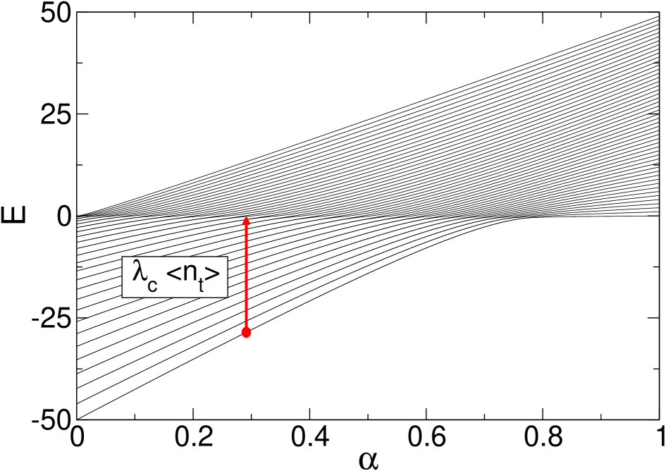
Figure 1: (Color online). Energy levels for the environment Hamiltonian (4) with $N=50$. The arrow (red online) shows the jump that the coupling with the central qubit produces in the environment.

To understand how this critical energy can be reached when we couple this environment to a central qubit let us take in consideration the following. We start the evolution with the ground state of the environment $\left|g_{0}\right>$. At $t=0$ we switch on the interaction between the system and the environment, and let the system evolve under the complete Hamiltonian. By instantaneously switching on this interaction, the energy of the environment increases, and its state gets fragmented into a region with average energy equal to $E=\left<g_{0}\right|H_{1}(\alpha)\left|g_{0}\right>$. Therefore, if $\left<g_{0}\right|H_{1}(\alpha)\left|g_{0}\right>=0$, the coupling with the central qubit induces the environment to jump into a region arround the critical energy $E_{c}$. This is illustrated in Fig. 1. Starting from a state in the parity broken phase with $\alpha<\alpha_{c}$, the coupling with the qubit, $H_{\lambda_{1}}=\lambda n_{t}$ increases the energy of the environment up to the critical point $E_{c}$. Resorting to the coherent state approach Vidal:06 , we can obtain a critical value of the coupling strength

$$\lambda_{c}(\alpha)=\frac{1}{2}\left(4-5\alpha\right),\;\;\;\alpha<\frac{4}{5}.$$ (7)

In Fig. 2 we show the modulus of the decoherence factor $\left|r(t)\right|$ for $\alpha=0$ and several values of $\lambda$ (see caption). In four of the five cases we can see a similar pattern, fast oscillations plus a smooth decaying envelope. For $\lambda\gtrsim\lambda_{*}$, this envelope is weakly dependent on $\lambda$. As we increase $\lambda$, the frequency of the short period oscillations increases linearly $\nu\approx\lambda/3$, but the main trend of the curve remains the same. The shape of the envelope can be fitted to a Gaussian decay for short times, and to a power-law decay for longer times; a similar behavior was identified in Paz:08 if the Hamiltonian parameter is close to or larger than the critical value. However, the most striking feature of Fig. 2 is the panel corresponding to $\lambda=2$, for which $\left|r(t)\right|$ quickly decays to zero and then randomly oscillates around a small value. We note that this particular case constitutes a singular point for both the shape of the envelope of $|r(t)|$ and the period of its oscillating part. Making use of Eq. (7) for $\alpha=0$ we obtain precisely $\lambda_{c}=2$, the value at which the coherence of the system is completely lost. Therefore, the existence of an ESQPT in the environment has a strong influence on the decoherence that it induces in the central system. We can summarize this result with the following conjecture:

If the system-environment coupling drives the environment to the critical energy $E_{c}$ of a continuous ESQPT, the decoherence induced in the coupled qubit is maximal.

Figure 2: $|r(t)|$ for $\alpha=0$ and five different values of $\lambda$. In all cases $N=10000$.

Let us check this conjecture for different values of $\alpha<\alpha_{c}=4/5$ . In Fig. 3 we show how the decoherence process changes around the critical value $\lambda_{c}$ for different values of $N$ and $\alpha$. As a representative quantity, we plot $r_{max}(\alpha)$ which is the value of $\left|r(t)\right|$ at the second maximum (the first maximum is $\left|r(0)\right|=1$ in all cases). We can extract two main conclusions from Fig. 3. First, $r_{max}(\lambda)$ is minimum at $\lambda\approx\lambda_{c}$, as given in Eq. (7) —the four cases plotted in the figure correspond to $\lambda_{c}=0.25,\,0.5,\,1.0,\text{ and }2.0$. Second, the behavior of this quantity is smooth and independent of the environment size $N$, except in a small region around $\lambda\approx\lambda_{c}$ where it becomes sharp and size dependent. Therefore, the decoherence factor behaves in a critical way around $\lambda=\lambda_{c}$ where $r_{max}(\lambda_{c})$ undergoes a dip towards zero which is sharper and deeper for larger values of $N$.

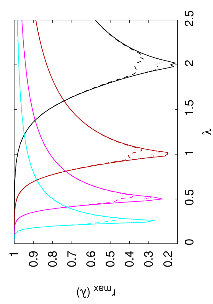
Figure 3: (Color online). $r_{max}(\lambda)$ in function of the coupling $\lambda$, for different values of $\alpha$ and $N$. Black lines represent the case $\alpha=0$; dark grey (red online) lines, $\alpha=0.4$; grey (magenta online), $\alpha=0.6$; and light grey (cyan online), $\alpha=0.7$. Solid lines represent $N=10000$; dotted lines, $N=2500$; and dashed lines, $N=600$.

Figure 4: $r_{max}(\lambda_{c})$ in function of the size of the environment $N$, in a double logarithmic scale. Squares represent the case $\alpha=0$; circles, $\alpha=0.4$; upper triangles, $\alpha=0.6$; lower triangles, $\alpha=0.7$. The straight lines correspond to a least squares fit to the power law $r_{max}(\lambda_{c})=AN^{-1/4}$.

On the light of these results, one may wonder how $r_{max}(\lambda_{c})$ behaves in the thermodynamical limit. As it is very difficult to do exact calculations beyond size $N>10000$, we will rely on the finite size scaling analysis to extrapolate its behavior for $N\rightarrow\infty$. In Fig. 4 we show how this quantity evolves with the size $N$ of the environment. We plot results for the same values of $\alpha$ as in Fig. 3 in a double logarithmic scale (see caption of Fig. 4 for details). In all the cases we obtain a power law $r_{max}(\lambda_{c})\sim N^{-\gamma}$, with $\gamma=1/4$.

The results displayed in figures 3 and 4 confirm that the presence of an ESQPT in the environment spectrum is clearly signaled by the qubit decoherence factor. Moreover, the quantity $r_{max}$ behaves in parallel way as the order parameter $n_{t}$ at the ESQPT Caprio:08 .

Prior to the conclusions, it is worth mentioning that the environmental Hamiltonian Eq. (4) is a particular case of a more generic class of two-level bosonic systems Vidal:06 , described by $H=\alpha n_{l}-(1-\alpha)\;Q^{(\omega)}_{l}\cdot Q^{(\omega)}_{l}/N$, with $Q^{(\omega)}_{l}=\left(s^{\dagger}\widetilde{l}+l^{\dagger}s\right)^{(l)}+\omega\left(l^{\dagger}\widetilde{l}\right)^{(l)}$, where the boson $s^{\dagger}$ is a scalar and the boson $l^{\dagger}$ has multipolarity $l$, as well as the operator $Q^{(\omega)}_{l}$ depending on an extra parameter $\omega$. As a representative case, we have presented here calculations using the environmental Hamiltonian with $l=0$ and $\omega=0$, characterized by a second order QPT. For $l>1$ this wide class of Hamiltonians, that have been extensively used in nuclear and molecular physics, present a richer structure with second order ($\omega=0$) and first order ($\omega\neq 0$) QPTs. A complete analysis on the influence of the order of the ESQPT in the decoherence process will be given in a future publication. Moreover, as the natural state of a realistic environment is a thermal one —that is, a mixed state in which the environment is in contact with a thermal bath characterized by a temperature $T$— it will be also interesting to check to which extent the temperature affects this critical behavior.

In this paper, we have studied the decoherence induced on a one-qubit system by the interaction with a two-level boson environment, which presents both a standard QPT and an ESQPT. Our main finding is that the decoherence is maximal when the system-environment coupling introduces in the environment the energy required to undergo a continuous ESQPT. The decoherence factor displays a critical behavior well described by $r_{max}(\lambda)$, the value of the second local maximum of $|r(t)|$. $r_{max}(\lambda)$ approaches zero for $\lambda\rightarrow\lambda_{c}$ in the thermodynamical limit showing a finite size scaling $r_{max}(\lambda_{c})\propto N^{-\gamma}$, with a critical exponent $\gamma=1/4$. Therefore, we conclude that the decoherence induced in a one-qubit system gives a unique signature of an ESQPT in the environment. Finally, let us point out that quantum decoherence could constitute an important tool to detect critical regions in the energy spectrum of mesoscopic systems; conversely, this knowledge could help to avoid certain environments that are particularly efficient to destroy quantum coherence. Moreover, as the particular Hamiltonian we have studied in this paper has been broadly applied in nuclear structure, molecular physics and, more recently, optical cavity QED, it is feasible to use any of these systems as the environment in a decoherence experiment.

This work has been partially supported by the Spanish Ministerio de Educación y Ciencia and by the European regional development fund (FEDER) under projects number FIS2005-01105, FIS2006-12783-C03-01 FPA2006-13807-C02-02 and FPA2007-63074, by Comunidad de Madrid and CSIC under project 200650M012, and by Junta de Analucía under projects FQM160, FQM318, P05-FQM437 and P07-FQM-02962. A.R. is supported by the Spanish program ”Juan de la Cierva”, and P. P-F., by a grant from the Plan Propio of the University of Sevilla.

References

- (1) W. H. Zurek, Rev. Mod. Phys. 75, 715 (2003).
- (2) M. Nielsen and I. Chuang, Quantum Computation and Quantum Information (Cambridge University Press, Cambridge, UK, 2000).
- (3) H. T. Quan, Z. Song, X. F. Liu, P. Zanardi, and C. P. Sun, Phys. Rev. Lett. 96, 140604 (2006).
- (4) F. M. Cucchietti, S. Fernandez-Vidal, and J. P. Paz, Phys. Rev. A 75, 032337 (2007).
- (5) C. Cormick and J. P. Paz, Phys Rev. A 77, 022317 (2008).
- (6) D. Rossini, T. Calarco, V. Giovannetti, S. Montangero, and R. Fazio, Phys. Rev. A 75, 032333 (2007).
- (7) P. Cejnar, S. Heinze, and M. Macek, Phys. Rev. Lett. 99, 100601 (2007).
- (8) P. Cejnar and J. Jolie, arXiv:0807.3467 (2008).
- (9) W. D. Heiss, F. G. Scholtz, and H. B. Geyer, J. Phys. A 38, 1843 (2005); F. Leyvraz and W. D. Heiss, Phys. Rev. Lett. 95, 050402 (2005); W. D. Heiss, J. Phys. A 39, 10081 (2006).
- (10) S. Heinze, P. Cejnar, J. Jolie, and M. Macek, Phys. Rev. C 73, 014306 (2006); M. Macek, P. Cejnar, J. Jolie, and S. Heinze, Phys. Rev. C 73, 014307 (2006); P. Cejnar, M. Macek, S. Heinze. J. Jolie, and J. Dobes, J. Phys. A 39, L515 (2006).
- (11) M. A. Caprio, P. Cejnar, and F. Iachello, Ann. Phys 323, 1106 (2008).
- (12) J. Vidal, J. M. Arias, J. Dukelsky, J. E. García-Ramos, Phys. Rev. C 73, 054305 (2006); J. M. Arias, J. Dukelsky, J. E. García-Ramos, and J. Vidal, Phys. Rev. C 75, 014301 (2007).
- (13) D. Bonatsos, E. A. McCutchan, R. F. Casten, and R. J. Casperson, Phys. Rev. Lett. 100, 142501 (2008).
- (14) F. Pérez-Bernal and F. Iachello, Phys. Rev. A 77, 032115 (2008); F. Pérez-Bernal, L. F. Santos, P. H. Vaccaro, and F. Iachello, Chem. Phys. Lett. 414, 398 (2005).
- (15) S. Morrison and A. S. Parkins, Phys. Rev. Lett. 100, 040403 (2008); Phys. Rev. A 77, 043810 (2008).