Computing Optimal Designs of multiresponse Experiments reduces to Second-Order Cone Programming
Abstract
Elfving’s Theorem is a major result in the theory of optimal experimental design, which gives a geometrical characterization of optimality. In this paper, we extend this theorem to the case of multiresponse experiments, and we show that when the number of experiments is finite, the and optimal design of multiresponse experiments can be computed by Second-Order Cone Programming (SOCP). Moreover, the present SOCP approach can deal with design problems in which the variable is subject to several linear constraints.
We give two proofs of this generalization of Elfving’s theorem. One is based on Lagrangian dualization techniques and relies on the fact that the semidefinite programming (SDP) formulation of the multiresponse optimal design always has a solution which is a matrix of rank . Therefore, the complexity of this problem fades.
We also investigate a model robust generalization of optimality, for which an Elfving-type theorem was established by Dette (1993). We show with the same Lagrangian approach that these model robust designs can be computed efficiently by minimizing a geometric mean under some norm constraints. Moreover, we show that the optimality conditions of this geometric programming problem yield an extension of Dette’s theorem to the case of multiresponse experiments.
When the goal is to identify a small number of linear functions of the unknown parameter (typically for optimality), we show by numerical examples that the present approach can be between 10 and 1000 times faster than the classic, state-of-the-art algorithms.
keywords:
Optimal design of experiments, Multiresponse experiments, optimality, optimality, SDP, SOCP, Convex optimization.1 Introduction
An important branch of statistics is the theory of optimal experimental designs, which explains how to best select experiments in order to estimate a vector of parameters . We refer the reader to the monographs of Fedorov [12] and Pukelsheim [24] for a comprehensive review on the subject, and to an article of Atkinson and Bailey [1] for more details on the early development of this theory.
The importance of Elfving’s Theorem (1952) [11], which was one of the first major improvements in the field of optimal design of experiments, was illustrated in many works [6, 7, 10, 13, 29, 31]. This result gives a geometrical characterization of the experimental design which minimizes the variance of the best estimator for the linear combination of the parameters . Namely, the optimal design can be found at the intersection of a vectorial straight-line and the boundary of a convex set referred as Elfving Set. When the number of available experiments is finite, Elfving set becomes a polyhedron, and so Elfving’s geometrical characterization allows one to compute optimal designs by linear programming methods, see Harman and Jurìk [14].
An interesting case appears in the study of the design of experiments, when a single experiment is allowed to give simultaneously several observations of the parameters. This setting is referred in the literature as multiresponse experiments, and occurs in many practical situations. For more details on the optimal design of multiresponse experiments, the reader is referred to the book of Fedorov [12].
In this paper, we extend Elfving’s classic result (Theorem 2.1) to the optimal design of multiresponse experiments, see Theorem 3.1, and we show that the latter problem reduces to a Second-Order Cone Programming problem (SOCP), see Theorem 3.3.
Moreover, we show in Section 4.1 that this result generalizes the Elfving-type result of Studden [29], which characterizes geometrically the optimal design for the estimation of a multidimensional linear combination of the parameters. As a consequence, one may cast the problem of finding an optimal design on a finite regression range (for single- or multi- response experiments) as an SOCP.
In contrast to the classic algorithms for the computation of optimal designs, the flexibility of mathematical programming approaches makes it possible to add constraints in the problem without additional effort. We will see that the present SOCP approach can indeed handle optimal design problems subject to multiple resource constraints, see Section 4.2.
The fact that the optimal design problem (on a finite regression space) has a semidefinite programming (SDP) formulation can be traced back to 1980, as a particular case of Theorem 4 in Pukelsheim [23]. Similarly, the classic A- and D- optimal design problems for multiresponse experiments can be formulated as SDP [34]. Second Order Cone Programming (SOCP) is a class of convex programs which is somehow harder than linear programming (LP), but which can be solved by interior point codes like SeDuMi [30] in a much shorter time that semidefinite programs (SDP) of the same size. Moreover the SOCP method takes advantage of the sparsity of the matrices arising in the problem formulation. Hence, this work shows that computing - and optimal designs actually belongs to an easier class of problems, and makes it possible to solve instances that were previously intractable.
While our proof of Theorem 3.1 is an extension of Elfving’s original proof, it leaves unexplained why the SDP formulation actually reduces to an SOCP. We provide in Section 5 another proof of the present Elfving-type result based on Lagrangian relaxation, which explains why the complexity of this problem fades. The proof relies on Theorem 5.2, which shows that a certain class of semidefinite programs (packing programs with a rank-one objective function) have a rank-one solution. Theorem 5.2 appears to be a result of an independent interest, in relation with the study of semidefinite relaxations of combinatorial optimization problems, and is therefore the subject of the companion paper [26].
We next show (Theorem 6.1) that optimality also admits a second order cone programming representation, which gives another argument for saying that second order cone programming is a natural tool for handling experimental optimal design problems. If the experimenter wishes to estimate the full vector of parameters , the optimal design problem is trivial. However, if he is interested in a linear subsystem , the optimal design problem is complicated and can be handled by SOCP.
In Section 7, we consider a generalization of optimality which was originally proposed by Läuter [17] in order to deal with the uncertainty on the model. In this approach (called optimality by Läuter), the objective criterion takes into account the variance of several estimators, balanced in a log term with coefficients which indicate the belief of the experimenter in each model. Dette [7] characterized by an Elfving-type result the optimal designs. We show in Theorem 7.1, which is the main result of this section, that when the number of available experiments is finite, optimal designs of multiresponse experiments can be computed efficiently by minimizing a geometric mean under some norm constraints. Moreover, we show in Theorem 7.3 that the optimality conditions of this geometric program yield an extension of Dette’s theorem to the case of multiresponse experiments. As a consequence of Theorem 7.1, we obtain a SOCP for optimality (cf. Remark 7.5). The results of this section are proved in appendix.
This work grew out from an application to networks [2], in which the traffic between any two pairs of nodes must be inferred from a set of measurements. This leads to a large scale optimal experimental design problem which can not be handled by standard SDP solvers. In a companion work relying on the present reduction to an SOCP [28], we illustrate our method by solving within seconds optimal design problems that could not be handled by SDP. In addition, the constraints of the SOCP formulation involves the observation matrices of the experiments, which happen to be very sparse in practice. This is in contrast with the information matrices involved in the SDP formulation (), which are not sparse in general. The present SOCP formulation takes advantage of the intrinsic sparsity of the data, and the instances can be solved very efficiently.
We present in Section 8 some numerical experiments for problems of the kind that arise in network monitoring, as well as classic polynomial regression problems. Our experiments show that the SOCP approach is well suited when the number of linear functions to estimate is small. For the case of optimality (only one linear function to estimate), we will see that solving the second order cone program is usually 10 times faster than the classic exchange or multiplicative algorithms, and up to 2000 times faster than the SDP approach for problems with multiple constraints.
Some results of this paper, including Theorem 3.1, were presented at the conference [27], and the technical result justifying the reduction to a SOCP was posted on arXiv [26]. Shortly before the time of submission, Dette and Holland-Letz published an article in Annals of Statistics, in which Theorem 3.1 was established independently (Theorem in [8]). Dette and Holland-Letz considered a heteroscedastic model (i.e. an experimental model where both the mean and the variance of the observations depend on the parameter of interest), which led them to study the case in which the observation matrices are of rank , just as in the model of multiresponse experiments. They used their geometrical characterization of the optimal design for heteroscedastic models in an application to toxicokinetics and pharmacokinetics. It should also be mentioned that the proof of Dette and Holland-Letz relies on an equivalence theorem (Theorem in [8]), while ours is closer to Elfving’s original approach, as done previously by Studden [31] for other results in optimal design of experiments. The main result of this article (reduction to a SOCP, Theorem 3.3), provides a new insight on the relations between these two approaches : they are actually dual from each other (in the Lagrangian sense). Indeed, the approach of Dette and Holland-Letz corresponds to the primal SOCP (8), while our geometrical characterization corresponds to the dual SOCP (9), and strong duality holds between these two optimization problems.
2 Preliminary results
Before stating the main results of this paper, we introduce the necessary background and recall Elfving’s classic result. Throughout this paper, we denote vectors by boldface letters and matrices by capital letters. We make use of the standard notation . The components of a vector are denoted by . The norm of is denoted by , and the Frobenius norm of a matrix by . The notation means that every component of is nonnegative.
The most common model in optimal experimental design assumes that each experiment provides a measurement which is a linear combination of the parameters up to the accuracy of the measurement. Let denote the set of available experiments. Every experiment provides a measurement
| (1) |
where is the dimensional vector of unknown parameters, and is the ()-regression vector. Uncorrelated experiments are performed at different locations from the compact set (possibly infinite), and the objective is to determine both the optimal choice of the , and the number of experiments to be conducted at ; we call such a subset of experiments a design.
Rather than deciding the exact number of times that each experiment should be conducted, it has been proposed to work with approximate designs instead, which is simply done by releasing the integrity constraints on the . In this setting, a mass indicates the proportion from the total number of experiments to be conducted for each available experiment. For example, if the weight for the experiment is , and that experiments are allowed, are chosen at . This definition suggests that the vector of weights is such that each quantity is integer. However, the continuous relaxation where every vector summing to is allowed is of theoretical interest. The approximate design where the percentage of experimental effort at is is written as
or for short. In this paper, we consider only approximate designs.
The celebrated result of Elfving [11] gives a geometrical characterization of the design (known as optimal) which minimizes the variance of an unbiased estimator for a single linear combination of the parameters. In this paper, we are going to extend Elfving’s Theorem to the multiresponse case. To this end, we consider the linear regression model
where is an unknown -dimensional parameter, is the -dimensional measurement vector for the experiment at , is a observation matrix, and is the error on the measurement. The matrix may eventually become rank deficient for certain values of . This allows one to handle the case in which the experiment at gives only measurements. In this case, we set rows of the matrix to zero.
The observations are uncorrelated and have a constant variance, which will be assumed to be one for the ease of the presentation, i.e.
In fact, one can always reduce to this case when the variance of the experiments is known, after a left scaling of the observation equations.
When experiments are conducted at , we denote by the average of these observations: we have , and . For the design , we denote by the aggregate vector of observations , and by the aggregate observation matrix , so that , and , where
| (2) |
with identity blocks on the diagonal. If for some , we simply remove the measurement point from . For ease of presentation, we get rid of the multiplication factor , since it does not affect the results on optimal designs.
Assume now that an experimenter wishes to estimate the scalar quantity , that is to say that he wants to estimate a linear combination of the parameters. It can easily be seen that a linear estimator is unbiased if and only if . Thus, linear unbiased estimators for exist as long as . We will say that the quantity is estimable when there is a design such that . Notice that a sufficient condition which ensures that is estimable for all is that the matrices contain linearly independent vectors among their rows. For an estimable quantity , we define the feasibility cone as the set of designs such that span the vector , and a design will be said feasible if it lies in the feasibility cone.
Now, let us assume that the quantity is estimable. Our protagonist certainly wants to choose an unbiased estimator of with minimal variance; the variance of is equal to , and we know from Gauss-Markov theorem that it is minimized under the unbiasedness constraint for , where denotes the Moore-Penrose pseudo inverse of , and the variance of this best linear unbiased estimator is :
where is a generalized inverse of , i.e. any matrix verifying . Notice that this expression does not depend on the choice of the generalized inverse , since there exists a vector such that :
The matrix is traditionally called the information matrix of the design, and it can be written as a weighted sum of the observation blocks :
| (3) |
In a more general setting, is replaced by a probability measure on :
However, this continuous form of the information matrix is still a symmetric matrix from the closed convex hull of . When is compact, and is continuous, the set of all information matrices is closed, and we know from Caratheodory’s theorem that can be written as barycenter of information matrices (see Fedorov [12]). Therefore, the optimal design can always be expressed with a discrete measure , where is the Dirac measure and . We will consider only such discrete designs in this work.
The optimal problem is to find the feasible design minimizing the variance of the aforementioned estimator:
| (4) | ||||
We point out that Problem (4) is not limited to the case of multiresponse experiments; there are other situations where the information matrix takes the form of Equation (3) (with ), for example in the case of models with parametrized variance or in models with correlated observations (see e.g. [19, 21]).
In the classic model (single response experiments), is a scalar observation, which means that and is a row vector. In this case, Elfving’s Theorem gives a geometrical characterization of the optimal design. We first define the Elfving set as the convex hull of the vectors :
and we denote its boundary by .
Theorem 2.1 (Elfving [11]).
A design is optimal if and only if there exists scalars and a positive real such that
Moreover, is the minimal variance.
Elfving’s theorem shows that the optimal design is characterized by the intersection between the vectorial straight line directed by and the boundary of the Elfving set . We also point out that when the vector is not spanned by the regression vectors , in other words when is not estimable (i.e. ), then the only scalar such that lies in is , and so a optimal design does not exist.
We show on Figure 1 a representation of Elfving’s theorem in dimension . Here, is finite, such that the Elfving set is a polyhedron. The vector is along the axis, which means that the experimenter wants to estimate . The intersection between this axis and the Elfving set indicates the optimal weights of the optimal design: and . Note that since is in the interior of the Elfving set, the experiment is never selected, whatever is the vector . This example also shows that the optimal design can be computed by linear programming (LP) when is finite (intersection of a straight line and a polyhedron). This feature was noticed by Harman and Jurík [14], who formulated the optimality LP:
| (5) | ||||
3 Extension to the case of multiresponse experiments
In this paper, we extend Elfving’s result to the case of multidimensional observations, by defining an analog of the Elfving set for the multiresponse case:
Following our proof, we further show in Theorem 3.3 that the optimal design of multiresponse experiments can be formulated as a Second Order Cone Program.
Theorem 3.1 (Extension of Elfving’s theorem for multiresponse experiments).
A design is optimal if and only if there exists a positive scalar and vectors in the unit ball of (i.e. ), such that
Moreover, is the minimal variance.
Proof.
We consider an unbiased linear estimator for :
The unbiasedness property forces the following equality to hold :
Now, the Cauchy-Schwarz inequality gives the following lower bound for the variance of :
| (6) |
where and was defined in Equation (2). We recall that we assume without loss of generality, since an experiment with a zero weight can be removed from the design .
We show that , by writing:
where and , so that , and .
Let be a positive scalar such that . The fact that implies
| (7) |
Combining (6) and (7) leads to the lower bound for the variance of any linear unbiased estimator of .
We will show that this lower bound is attained if and only if the design satisfies the condition of the theorem. To do this, notice that for a design and an estimator to be optimal, it is necessary and sufficient that the inequalities (6) and (7) are equalities. The Cauchy-Schwarz inequality (6) is an equality if and only if is proportional to the vector i.e.
The second inequality (7) is an equality whenever , i.e. where is the largest real such that . We can write
with and . We have , and the equality conditions are satisfied if and only if . ∎
Remark 3.2.
The latter theorem has a simple geometric interpretation. In the scalar case, we have seen that the optimal design could be find at the intersection of a polyhedron and a straight line directed by (see Figure 1). In the multiresponse case, the generalized Elfving set is no longer a polyhedron: instead, we compute the intersection between the straight line directed by and the set
where is the ellipsoid with semi-axis (), where are the eigenvalues of and are the corresponding eigenvectors. In the common case, we have , such that some eigenvalues of vanish and the ellipsoid is not full-dimensional (i.e. its volume is zero). We illustrate this geometric interpretation in Figure 2. Moreover, we see in next theorem that the intersection which characterizes the optimality can be computed by a Second order cone program.
Theorem 3.3 (Computation of the optimal design by SOCP).
Assume that the number of available experiments is , so that can be identified with . Let be a pair of primal and dual solutions of the second order cone programs:
| (8) | ||||
| (9) | ||||
We define
Then is a optimal design. Moreover, is the best linear estimator of , and the optimal variance is .
Proof.
This result is actually a corollary of Theorem 3.1. As in the proof of the latter theorem, define as the largest scalar such that , i.e. such that there exists summing to and vectors in the unit ball of satisfying
This decomposition gives the optimal weights and the best estimator of :
| (10) |
where . According to the proof of Theorem 3.1 indeed, an unbiased estimator of the form (10) is optimal if and only if every is proportional to and has norm . Setting , one obtains as the value of the following SOCP:
| (11) | ||||
In order to get an SOCP in the standard form, we write , where is an arbitrary nonnegative scalar. Then, we set , and we obtain a problem in the form of (9). Finally, the value of and are equal, since the Slater condition holds for this pair of programs (the dual is strictly feasible and the primal is feasible). A proof of the strong duality theorem for SOCP can be found e.g. in [20], Section 4.2. See [18] for more background on SOCP duality theory. ∎
The previous theorem shows how one can compute the optimal design on a finite regression region by solving an SOCP. This can be done with the help of interior points codes such as SeDuMi [30]. Solving the latter SOCP (8) is a much easier task than solving the former state-of-the-art SDP for optimality, because the number of variables is in the order of (instead of ); because we have get rid off the positive semidefiniteness constraint of the SDP; and because the SOCP solver is able to exploit the sparse structure of the observation matrices (while the partial information matrices involved in the SDP are not very sparse in general. As stated in the introduction, this approach has been used for the computation of optimal designs for a network application [28]. Very large instances of experimental design problems arise for the optimal monitoring of IP networks indeed, and we will see in Section 8.3 that the present SOCP can handle them.
4 Two extensions of the main result
In this section, we show that optimal designs can be computed by SOCP in two particular situations which generalize optimality, namely when the experimenter wants to estimate several quantities and chooses the optimality criterion, and when the design is subject to multiple resource constraints.
4.1 The case of optimality
When there are several quantities of interest, i.e. when consists in a collection of linear combinations of the parameters ( where is the matrix formed by the columns ), it is known that the best linear unbiased estimator is
and its covariance matrix is
Notice that an interesting case occurs when , i.e. when the experimenter wants to estimate the whole vector of parameters. As in the case of optimality, we say that is estimable if there is a design such that , and we denote by the feasibility cone (i.e. the set of designs satisfying the latter range inclusion).
The objective is now to minimize, in a certain sense, the variance of this best estimator. A widely used criterion is to minimize the trace of this matrix : such a minimizing design is known as optimal.
| (12) | ||||
We show in this section that computing the optimal design for the parameter of interest can be written as a optimal design problem with multidimensional observations. The objective function of (12) can indeed be written as
We define the vector as the vertical concatenation of the columns , i.e. . Now , we have: where:
In the latter equation, contains blocks and is of dimension . We can now rewrite Problem (12) in the following form:
We have thus shown that the problem of finding the optimal design is nothing but a optimal design problem, with augmented observation matrices . As a consequence, the results of Section 3 on optimality also apply for the more general optimal design problem for a subsystem of the parameters. In particular, the optimal design problem reduces to an SOCP:
Theorem 4.1 (Computation of the optimal design by SOCP).
Let be a pair of primal and dual solutions of the second order cone programs:
| (13) | ||||
| (14) | ||||
We define
Then, is optimal for . Moreover, is the best linear unbiased estimator of , and the optimal criterion is
We further show that the geometrical characterization of optimality for multiresponse experiments generalizes the result of Studden [29], who established an Elfving-type result for optimal designs of single-response experiments ( and is a row vector). This characterization is based on the following extension of the Elfving set when the matrix is :
Theorem 4.2 (Studden,1971).
A design is optimal for if and only if there exists a scalar and vectors in the unit ball of such that
Moreover, is the optimal value of the criterion.
One can easily verify that this theorem is a particular case of Theorem 3.1. Using the previously introduced notation indeed, Theorem 3.1 says that is optimal for if and only if there exists a scalar and vectors in the unit ball of such that
and we notice that is the vectorized version of , and when , is the vectorized version of and is the vectorized version of .
4.2 Optimal designs subject to multiple resource constraints
The great advantage of the mathematical programming formulations (LP,SOCP,SDP,…) resides mostly in their flexibility, and the possibility to add “without effort” new constraints in the problem. Elfving studied the case in which the available experiments have different costs [11]. If the cost of the experiment is , and the experimenter disposes of a budget , the constraint becomes:
Now, can not be interpreted as the percentage of experimental effort to spend on the experiment anymore. Instead, the quantity should be seen as the percentage of budget to allocate to the experiment . Elfving noticed that the change of variable brings the problem back to the standard situation, and is equivalent to a scaling of the observation equations (1).
Consider now the more general case in which is a control variable for the experiments, such that the information matrix takes the standard form for some observation matrices . We assume that is constrained by several linear inequalities
| (15) |
where is a matrix and the inequality is elementwise. Contrarily to the previous situation with a single budget constraint, there is no simple change of variable which brings the problem back to the standard case (), because we do not know which inequalities will be saturated in (15) at optimality. This constrained problem has been studied by Cook and Fedorov [5], who proposed an extension of the Fedorov exchange algorithm. However, the latter exhibits a slow convergence in practice.
This constrained framework arises in the problem of optimally setting the sampling rates of a measuring device on a network. In this case, is the vector of the sampling rates of the monitoring tool at different locations of the network, and the constraint reflects the fact that only a certain number of packets should be sampled at each router [28]. Another example of application of optimal design problems with multiple constraints was given by Vandenberghe, Boyd and Wu [34]: they have shown that constraints of the form (15) can be used to avoid concentrated designs. For example, we can impose that no more than a given fraction of the experimental effort, say , is concentrated on a small number of experiments, say of the possible observations.
Adding those multiple resource constraints in the SDP formulation of the optimal design problem is straightforward. Doing the same thing for the SOCP formulation is a little more tricky, since some hyperbolic constraints need be reformulated as conic constraints. We do this in the next theorem. A related result was obtained by Ben-Tal and Nemirovskii [3], for an application to truss topology design (see also [20, 18]). Our statement of the theorem shows that the optimal variables of the SOCP moreover give the best estimator of and that the result holds even if the optimal information matrix is singular (but contains in its range).
Theorem 4.3.
The following SOCP is feasible if and only if is estimable for a feasible design (i.e. and ).
| (16) | ||||
| (19) |
If the latter SOCP moreover admits a solution , then is optimal (in the sense of the general problem with constraints ), the best unbiased linear estimator of is , and the optimal variance is .
Proof.
Let be a feasible design (). The Gauss Markov Theorem allows us to rewrite the objective criterion of the optimal design problem as:
| (20) | ||||
where is defined in Equation (2), and the optimal vector in this problem defines the best linear unbiased estimator of . Decomposing as , the expression can be rewritten as
| (21) |
Recall that when an experiment is unobserved (), it could simply be removed from the support of the experimental design. In other words, the sum (21) is taken on the indices such that only. We can now rewrite the optimal design problem with constraints in a form that involves the vector of coefficients of the estimator :
| (22) | ||||
Clearly, this is equivalent to:
| (23) | ||||
since we can assume without loss of generality that . Finally, the SOCP (16) is obtained by reformulating the hyperbolic constraints as
We now show that Problem (23) is feasible if and only if the quantity is estimable for a feasible design. We first assume the contrary, i.e. . Let satisfies the inequality constraints; we denote by the subset of indices such that , so that we have
Now, if for some vectors , it implies that for an index such that , and the hyperbolic constraint is violated. Conversely, let be a feasible design, and defined as above. Since we can write for some vectors . Finally, we define for all , and for all the other indices : Problem (23) is feasible for the vectors and . However, we point out that Problem (23) (as well as the optimal design problem with multiple constraints) may fail to have a solution when the polyhedron is not bounded, because in some cases the minimum is not attained and the infimum can be approached by a sequence of designs such that . ∎
5 Alternative approach via Lagrange duality
The aim of this section is to prove directly the equivalence between Problem (4) and the Second Order Cone Programs (8)-(9) by use of Lagrangian duality tools, when the number of available experiments is finite (or equivalently that the locations of the selected experiments are given in advance). As stated in the introduction, the motivation for this work is to understand why the former SDP approach of this problem actually reduces to a much easier problem. Moreover, our proof handles the multiresponse case in the same manner as the single-response case, by simply substituting observation row vectors with observation matrices in the constraints of the optimization problem, and it can be applied in a more general framework (cf. Section 7).
We first recall that the optimal design problem (4) is equivalent to a semidefinite program. The optimality SDP already appeared in Pukelsheim [23], hidden under a more general form. The proof given in this paper is more elementary, and it can be adapted to handle optimality (cf. Lemma A.1). In the sequel, denotes the Löwner ordering of symmetric matrices, that is, if and only if is positive semidefinite.
Theorem 5.1.
When the regression range is finite (), the optimal design problem (4) is equivalent to the following pair of primal and dual SDP. More precisely, let be a pair of primal and dual solution of the SDPs:
| (24) | ||||
| s.t. | ||||
| (25) | ||||
| s.t. |
Then, the vector is solution of the optimal design problem (4), and the following relation holds:
Proof.
Since the feasible designs must be such that , we can write, using a generalized Schur complement:
for . Note that if we exclude the trivial case , we can always assume that . So, the optimal design problem (4) can be rewritten as:
| (26) | ||||
| s.t. | (29) | |||
Now, we re-express the positive-semidefiniteness of the matrix in (26) with another Schur complement:
Setting the new variable , so that , we obtain a semidefinite program in the form of . Strong duality holds between and , because the Slater condition for semidefinite programming is satisfied (the primal problem is strictly feasible, and its dual is feasible). Finally, notice that the dual feasibility condition implies that is included in , so that we do not have to worry about the the constraint in the initial problem (4). ∎
We notice that when the above SDP has a rank one solution, it can be reduced to the primal SOCP (8). The next theorem shows that such a rank-one solution always exists indeed, and its proof can be found in [26]. Note that this theorem is of independent interest. The general result establishes the existence of rank- solutions for the class of semidefinite packing problems in which the matrix defining the objective function has rank :
Theorem 5.2 (Low rank reduction theorem for semidefinite packing problems [26]).
Denote by the space of symmetric matrices, equipped with the inner product . We consider the following semidefinite packing program
| (30) | ||||
This problem is feasible if and only if every is nonnegative, and is bounded if and only if . Under these two conditions, the SDP (30) has a solution which is of rank at most .
In particular, if is a vector (i.e. ), then there is an optimal variable in the form for some vector , and is the solution of the following Second-Order Cone Program:
| (31) | ||||
| s.t. |
This theorem shows that if is estimable, then Problem (24) admits a solution of rank-one and reduces to Problem (8). This is another proof of Theorem (3.3) which explains why optimal designs can be computed by SOCP. To our sense, this proof gives a better understanding on how the computing gap from SDP to SOCP is crossed : the intrinsic positive semidefiniteness of the data in the SDP ensures that there is a solution of rank , which explain why the complexity of the problem fades.
Remark 5.3.
Remark 5.4.
The theorem above can be extended to a semi-infinite programming context. This allows one to write the optimal design problem over an infinite regression region under the form:
| (32) | ||||
Note that this formulation is given with a theoretic purpose only, since the resolution of this kind of problem is very hard, even in the case in which is linear in . If some regularity conditions are satisfied by the application , then there is a stochastic algorithm which converge to the optimal of Problem (32) with probability [33], but the convergence can be extremely slow. If we can solve this optimization problem, though, then the points where the inequality constraint is active are nothing but the support of the optimal design.
6 T-optimality for
When several quantities are of interest (optimal design for ), another classic criterion from the experimental design literature is the optimal design problem:
| (33) | ||||
| s.t. |
The criterion can be extended by continuity to the designs such that is not invertible, i.e. such that . Contrarily to the optimality criterion, there are some examples where the maximum is attained for a nonfeasible design (see Pukelsheim [24], Section 6.5). Following the terminology of Pukelsheim, we call a design formally optimal if it maximizes the objective criterion subject to the constraints only, i.e. when we ignore the feasibility condition . Note that a formally T-optimal design always exists, because the feasibility region becomes compact when we remove the feasibility constraint. Pukelsheim shows in Section 9.15 of [24] that the optimal design problem for the full parameter is trivial: if is estimable (), then a design is formally optimal for if and only if it allocates all the weight to the experiments such that is maximal. However, when the quantity of interest is a parameter subsystem , , the problem becomes computationally challenging.
We show in this section that it is possible to compute a formally optimal design for with a SOCP when is finite. This gives another example of optimal experimental design problem which can be handled via Second Order Cone Programming.
Theorem 6.1 (T-optimality SOCP).
Let be finite, be an estimable quantity, and be a pair of primal and dual solutions of the second order cone programs:
| (34) | ||||
| (35) | ||||
(Note that these are Second Order Cone Programs indeed; we have let the hyperbolic constraints to simplify the notation, otherwise the matrices and need be vectorized). Then, is formally optimal for , and the value of the supremum in Problem (33) is . If moreover , then is optimal.
Proof.
Our proof relies on the general definition of the information matrix for , which is given by Pukelsheim in Chapter 3 of [24]:
| (36) | ||||
In the latter expression, the minimum is taken with respect to the Löwner ordering. Pukelsheim shows that the minimum exists indeed (which is not obvious since the Löwner ordering is a partial ordering), as a consequence of the Gauss-Markov Theorem (cf. Theorem 1.21 in [24]), and moreover that coincides with the standard expression for feasible designs .
Now, since the trace of a matrix preserves the Löwner ordering, we can express the (formal) optimal design problem as the following saddle point problem:
The exchange of the max and the min above is a consequence of Sion’s minimax theorem ( is continuous, concave in and convex in ). We next introduce a variable which must be larger than all the quantities , and we have shown that the (formal) optimal design problem for is equivalent to Problem (34). The (formal) T-optimal design is the optimal dual variable corresponding to the hyperbolic constraints in Problem (34). It follows that can be computed by solving the dual optimization problem (35). Finally, the value of these optimization problems is the same by Strong duality (Slater condition holds), and is equal to the optimum of the optimal problem (33).
∎
7 Convex optimization and optimality
The -criterion was introduced by Läuter [17] in order to tackle the uncertainty of the experimenter on the true model, by considering a class of plausible models with means
in which the quantity to estimate is .
In other words, the measurement at is modeled as a linear function of the parameter , which depends on the model, and must be used to estimate a linear function of the parameter in each model. In practice, the parameters of each of these models may be different. This can be handled by setting the column of to whenever the model at does not depend on . Note that we write the index of the model in parenthesis, in order to avoid ambiguities with the index of the experiment.
Given a nonnegative vector of size with sum , where indicates the importance that the experimenter attaches to the model , or the importance of the linear combination , the criterion is:
where
is the information matrix in the model. A design minimizing this criterion is called optimal. An interesting case occurs when the models are identical. This is an alternative approach to the optimality for , with weightings on each linear combination to be estimated. Dette studied the difference between these two approaches in Section 4 of [7].
We are next going to show that the optimal design of multiresponse experiments reduces to the problem of maximizing a weighted geometric mean under norm constraints. This is of great interest for the computation of optimal designs. Indeed, this optimization problem is a geometric program, and so it can be reformulated in a form for which a self-concordant barrier function is known, and it can be solved efficiently to the desired precision by interior point techniques (see e.g. [4]).
Theorem 7.1.
Let be a solution of the following optimization problem. Then, also minimizes the criterion. Moreover, the value of this program coincides with the value of its dual, which we give below.
| () | ||||
| (40) | ||||
| () | ||||
| (44) |
The variables of the primal optimization problem are (the design), and the vectors , for and . The variables of the dual problem are the vectors .
Remark 7.2.
The primal problem () is equivalent to maximizing the geometric mean under the same constraints, by monotonicity of the log function. Therefore, if is rational and the least common denominator of the is , we can reformulate Problem () as a SOCP by introducing less than additional norm constraints (cf. Section 6.2.3 of [20] or [18]).
The proof of Theorem 7.1 relies on a series of reformulations of the the optimal problem, relying on Lagrange duality techniques and Theorem 5.2. We will prove this result in appendix.
Then, we will show that the optimality conditions of the present convex optimization problem can be interpreted as geometrical conditions, which yields a generalization of the theorem of Dette for optimality to the case of multiresponse experiments [7]. This geometrical characterization relies on the following Elfving-type set:
Theorem 7.3 (Geometrical characterization of multiresponse optimality).
The design is optimal (and solution of Program ) if and only if there exists a vector and vectors (), such that
-
(i)
-
(ii)
-
(iii)
lies on the boundary of , with a supporting hyperplane whose normal direction is given by the matrix with . In other words,
-
(iv)
satisfies the equalities
In this case, the optimal variables of Problems and are , and , so that the optimal criterion is .
Theorem 7.3 is established in appendix.
Remark 7.4.
As in the case of single response experiments [7], the geometrical characterization remains true when the regression range is infinite. It can also be shown with semi-infinite programming techniques that the following convex semi-infinite program is valid for the general optimal design Problem:
Remark 7.5.
Dette showed in [7] that optimality for the full parameter is a particular case of optimality. As a consequence, we can formulate the optimal design problem as a convex optimization problem in the form of . To see this, Dette considered the virtual nested models, where the parameter of interest in the model is , and the observations only depend on the first parameters: is the matrix restricted to its first columns, so that is the upper left submatrix of , and is a vector of length . Using the relation
it can be seen that
which is exactly the optimality criterion.
Theorem 7.1 can now be used to formulate the optimal design problem as:
| (45) | ||||
| (49) | ||||
As pointed out in Remark 7.2, this optimization problem can be reformulated as a SOCP by introducing additional norm constraints, where is the smallest power of two that is greater or equal to .
8 Numerical Experiments
In this section, we evaluate the benefits of the SOCP approach for the computation of optimal experimental designs. We will see that the second order cone programs presented in this paper are very efficient when the number of quantities to estimate is small (in particular for optimality).
We will compare the SOCP approach approach to the semidefinite programming/MAXDET approach [34], and to other classic algorithms from the experimental design literature. We concentrate on Wynn–Fedorov-type exchange algorithms, and Titterington-type multiplicative algorithms. The former were discovered independently by Wynn [35] and Fedorov [12], and consist in moving at each step toward the experiment with the largest directional derivative. Several versions and refinements of this procedure were proposed; we will use the IncDec procedure of Richtarik [25], which specifies step lengths for which the precision is achieved in iterations.
On the other hand, multiplicative weight algorithms were introduced in 1976 by Titterington [32]. The monotonic behavior of any sequence generated by this algorithm was recently proved by Yu [36], for a large class of design criteria, including and optimality. We will also consider a variant of the latter algorithm, for which Dette, Pepelyshev and Zhigljavsky [9] have established a convergence result in the case of optimality, and conjectured the convergence for other criteria. These multiplicative algorithms use respectively a power parameter and an acceleration parameter . We found that the values and gave the best results for optimality in our experiments, and so those values will be used throughout this section. For optimality, we have used the acceleration parameter .
| SOCP (13) | SDP | IncDec Exchange | Accelerated Mult. | Mult.Weight with | |
|---|---|---|---|---|---|
| [this paper] | [34] | [25] | Weight () [9] | Exponent [36] | |
| failed | |||||
| failed | |||||
| failed |
We will first consider random instances of optimal design problems, in order to evaluate to which extent each parameter affects the computation time. Then, we will consider a simple polynomial regression model, for which we shall see that the SOCP approach is well-suited when the number of support points is large. Finally we will present some results from a network application – which is at the origin of this work– where the sampling rates of a monitoring tool should be optimized subject to multiple constraints.
8.1 Random instances
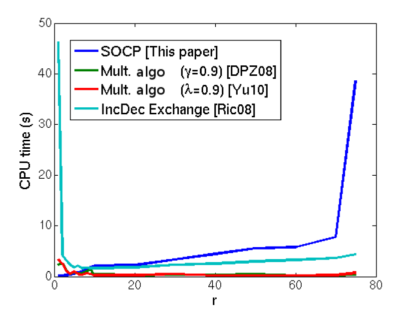
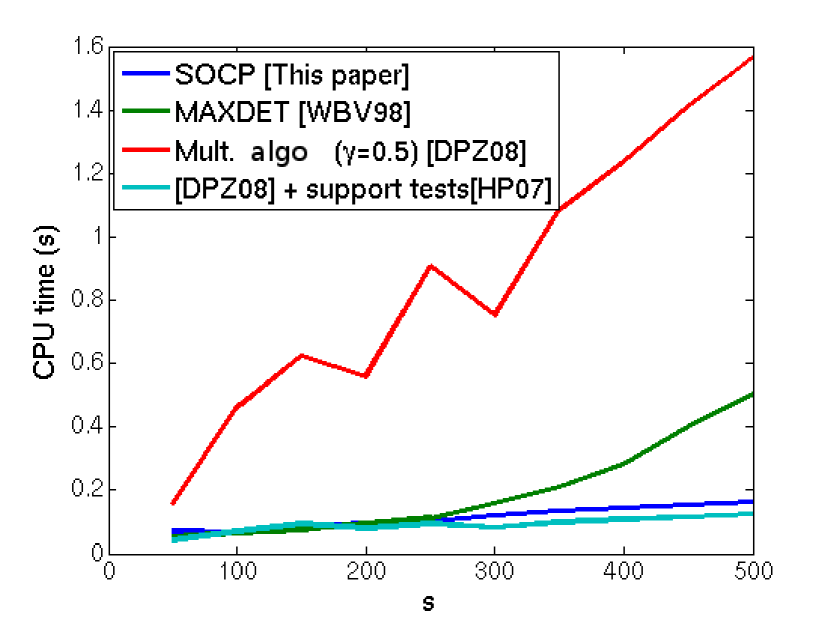 Figure 5: Comparison of four algorithms on typical random instances of the minimum covering ellipsoid (optimality for , ) and varying .
In this section, we consider random instances of optimal experimental design problems, in which the entries of the matrices follow a normal distribution, as well as the entries of the matrix . For every considered instance, we use SeDuMi to solve the SOCP (13) and the optimality SDP [34]; we have implemented the other procedures in Matlab. In all our experiments, the stopping criterion is based on the general equivalence theorem of Kiefer [16]: the computation stops as soon as the ratio between the maximum of the gradient and the value of the criterion is below 1.001 (as in [9]).
We start by evaluating the effect of , which turns out to be the determining factor for the performance of the SOCP approach. To this end, we set , , (single-response experiments), and we let vary between and . The computing time of the different algorithms is plotted against in Figure 5. We notice that the SOCP is the fastest for small values , but performs badly when is large, while the multiplicative weight algorithms are insensitive to the value of . For this reason, we will chose small values of in further experiments, since the SOCP approach might not be well adapted for large .
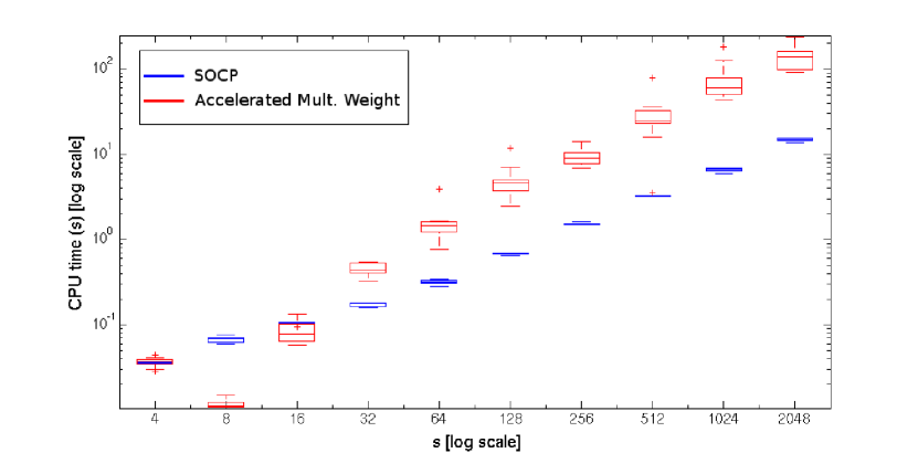
We next study the effect of (the number of available experiments) for the case of optimality (). For these experiments, we set , , and we take in the set . The performance (in terms of CPU time) of the SOCP is compared to that of the accelerated multiplicative algorithm (for , [9]) on the log-log plot of Figure 3. The boxes represent the distribution of the CPU time, on randomly generated instances. We see here that the SOCP approach is in average ten times faster as soon as .
To evaluate the effect of , we set , , , and choose in the set (Note that since and is randomly generated, we must have for the instance to be feasible). The results of each algorithm are displayed in Table 1. It is striking that the SOCP approach is the best one, while the SDP is the worst when becomes large, which demonstrates the importance of the rank reduction discussed in Section 5. For , the SOCP is 10 times faster than all other algorithms. In the last row of the table however, this ratio is lower. This might be because in this case, such that all experiments are support points of the optimal design, and classic algorithms certainly take advantage of this situation (while it does not make a difference for interior point codes).
Pronzato [22] has shown that we can improve the multiplicative algorithms thanks to a simple test which allows to remove on the fly experiments which do not belong to the optimal design (i.e. with a zero weight), and which was refined by Harman and Pronzato [15]. This can considerably improve the performance of the multiplicative algorithms when there are a lot of points with a zero weight. As in [15], we have studied random instances of the minimum covering ellipse, but in : , , and we draw independent random regression vectors () from a normal distribution , with increasing from to . The optimal design problem is equivalent to finding the minimum volume ellipsoid which contains the vectors , and the optimal design is supported by points lying on the boundary of this minimal ellipsoid. In accordance with intuition, the number of support points of the optimal design is small, and therefore the test of Pronzato and Harman improves dramatically the computing time (cf. Figure 5). Note however that the SOCP for optimality (45) remains competitive with the latter approach.
8.2 Polynomial Regression
We have computed the and -optimal designs (for the full parameter ), for a polynomial regression model of degree :
on the regression region . The optimal designs are represented on Figure 6. In this problem, we have , which is small. Therefore, we can hope that the SOCP approach will perform well. The computation times are plotted on Figures 8 and 8, as a function of the number of points considered for the discretization of the regression interval . For the optimal design, the experimental setting was the same that the one of previous section. For the optimal design problem, we solved the geometric program (9) with SeDuMi. We have also implemented the classic multiplicative algorithm, the accelerated algorithm with , and the MAXDET program [34]. Contrarily to the multiplicative algorithms, the interior point algorithms (SOCP and MAXDET) seem to be insensitive to the size of the discretization grid. For these instances, the SOCP is roughly two times faster than the MAXDET program. Also note that the effect of the acceleration parameter is clearly visible (red curve vs. green curve). We point out that for these polynomial regression problems, the tests of Pronzato and Harman [22, 15] to remove points that do not belong to the support of the optimal design did not yield any improvement.
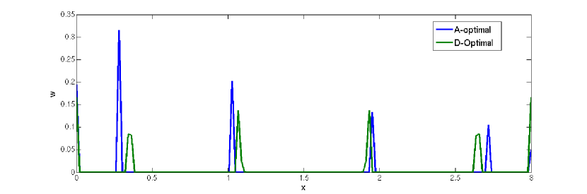
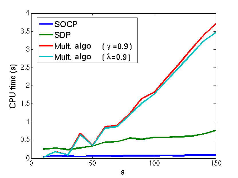
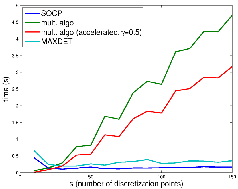 Figure 8: D-optimal design for the polynomial regression model: evolution of the computation time with the number of points
for the discretization of .
Figure 8: D-optimal design for the polynomial regression model: evolution of the computation time with the number of points
for the discretization of .
8.3 Optimal Sampling in IP networks
We finally show some results for an application to the optimal monitoring of large IP networks. Assume that an Internet provider wants to estimate the traffic matrix of his network, that is, the volume of traffic between each pair of origin and destination during a given time period. To this end, he disposes of a monitoring tool, which can be activated at different sampling rates in different location of the network, and is able to find the destination of the sampled packets. For networking issues, the intensive use of this tool is not suitable, because it creates an overload both in terms of CPU utilization of the router and bandwidth consumption. The sampling rates should therefore be tuned cautiously on each interface, in such a way that the number of sampled packets remains under a target threshold.
This situation can be represented by an optimal design model with multiresponse experiments: the set of available experiments coincides with the interfaces of the network where the monitoring-tool can be activated: when the software is installed on a given interface, we obtain an estimation of the sum of the flows that traverse this interface, and that have destination , for every destination reachable from this interface. In [28], two coauthors and I have shown that if the sampling rates are small, then the Fisher information matrix of the sampling design has the standard form (3) (after an appropriate normalization of the observation matrices relying on a prior estimate of the unknown OD traffic matrix). The optimal monitoring problem can thus be formulated as an optimal experimental design problem with multiple resource constraints.
We first study some optimal sampling problems with the simple constraint , so that we can compare the present SOCP approach to classic algorithms. Table 2 summarizes the results (in terms of CPU time) for several problems: each instance is defined by a network and the type of interfaces considered. We used the topology of three networks: Abilene, which consists in nodes, OD pairs and links; the Opentransit backbone of France Telecom, with nodes, OD pairs and links; and a clustered version of the latter network, thus reduced to nodes, OD pairs and links. The natural problem is to activate the monitoring tool independently on each link (interface=“links”). However, we also considered the academic problem of imposing the same sampling rates on all incoming links of each router, which is equivalent to consider each router as a big interface (interface=“Nodes”). For all these instances the vector was drawn from a normal distribution. The threshold for the stopping criterion was lowered to for this network application, since this value suffices to obtain good designs in practice.
| Network | Abilene | Abilene | OTClusters | OTClusters | Opentransit | Opentransit |
|---|---|---|---|---|---|---|
| () | () | () | () | () | () | |
| Interfaces | Nodes | Links | Nodes | Links | Nodes | Links |
| () | () | () | () | () | () | |
| SOCP | ||||||
| SDP | failed | failed | ||||
| IncDec Exchange | failed | failed | ||||
| Mult. algo () | failed | failed | ||||
| Mult. algo () | failed | failed |
We can see in the table that the multiplicative algorithms perform better than the SOCP approach on the instances where is small (1st and 3rd columns in Table 2). On the other instances however, the SOCP performs well, and it is the only method which returned a solution for the Opentransit network. The SDP and the multiplicative methods failed because of memory issues (in the multiplicative algorithm, a full rank update of the information matrix should be carried out at each time step). The IncDec Exchange algorithm did not crash, but it had not converged after 2 hours of computation.
We next turn to the case of general constraints of the form . Since we do not know any other algorithm which can handle optimal design problems with multiple resource constraints, we compare the SOCP and the semi-definite programming approaches only. Table 3 summarize the results (in terms of CPU time) for several problems, specified as previously by the network and the type of interfaces considered, and also by the type of the constraint matrix . In the optimal sampling problem, the matrix usually depends on the volume of traffic observed at each router (cf. [28]). We simulated this data from a uniform distribution, a lognormal distribution, or we used real traffic loads. To see the effect of the number of constraints, we also generated arbitrary constraints matrices of different sizes.
In comparison to the SDP, the computation time can be reduced by a factor in the order of on the instances from the clustered network. Moreover, the SOCP approach is able to handle huge instances arising from the Opentransit network (in which ).
| Network | Abilene | Abilene | Abilene | Abilene | Abilene |
|---|---|---|---|---|---|
| () | () | () | () | () | |
| Interfaces | Links () | Links () | Links () | Nodes () | Nodes () |
| Constraints | R: | R: | R: | R: | R: |
| (uniform traffic) | (lognormal traffic) | (real traffic) | (arbitrary) | (arbitrary) | |
| SOCP | |||||
| SDP | |||||
| Network | OTClusters | OTClusters | OTClusters | Opentransit | Opentransit |
| () | () | () | () | () | |
| Interfaces | Nodes () | Links () | Links () | Links () | Links () |
| Constraints | R: | R: | R: | R: | R: |
| (arbitrary) | (uniform traffic) | (arbitrary) | (arbitrary) | (real traffic) | |
| SOCP | |||||
| SDP | failed | failed |
9 Acknowledgment
The author is immensely grateful to Stéphane Gaubert, whose comments, advice and support were essential. He also wants to thank Mustapha Bouhtou for the stimulating discussions which are at the origin of this work. He also expresses his gratitude to two anonymous referees for their constructive comments, and more particularly to a referee who gave precious suggestions for the presentation of these experimental results.
References
- AB [01] A.C. Atkinson and R.A. Bailey. One hundred years of the design of experiments on and off the pages of Biometrika. Biometrika, 88(1):53–97, 2001.
- BGS [08] M. Bouhtou, S. Gaubert, and G. Sagnol. Optimization of network traffic measurement: a semidefinite programming approach. In Proceedings of the International Conference on Engineering Optimization (ENGOPT), Rio De Janeiro, Brazil, 2008. ISBN 978-85-7650-152-7.
- BTN [92] A. Ben-Tal and A. Nemirovskii. Interior point polynomial-time method for truss topology design. Technical report, Faculty of Industrial Engineering and Management, Technion institute of Technology, Haifa, Israel, 1992.
- BV [04] S. Boyd and L. Vandenberghe. Convex Optimization. Cambridge University Press, 2004.
- CF [95] D. Cook and V. Fedorov. Constrained optimization of experimental design. Statistics, 26:129–178, 1995.
- Che [99] H. Chernoff. Gustav Elfving’s impact on experimental design. Statistical Science, 14(2):201–205, 1999.
- Det [93] H. Dette. Elfving’s theorem for D-optimality. The Annals of Statistics, 21:753–766, 1993.
- DHL [09] H. Dette and T. Holland-Letz. A geometric characterization of c-optimal designs for heteroscedastic regression. The Annals of Statistics, 37(6B):4088–4103, December 2009.
- DPZ [08] H. Dette, A. Pepelyshev, and A. Zhigljavsky. Improving updating rules in multiplicative algorithms for computing D-optimal designs. Computational Statistics & Data Analysis, 53(2):312 – 320, 2008.
- DS [93] H. Dette and W.J. Studden. Geometry of E-optimality. The Annals of Statistics, 21:416–433, 1993.
- Elf [52] G. Elfving. Optimum allocation in linear regression theory. The Annals of Mathematical Statistics, 23:255–262, 1952.
- Fed [72] V.V. Fedorov. Theory of optimal experiments. New York : Academic Press, 1972. Translated and edited by W. J. Studden and E. M. Klimko.
- HHS [95] H.Dette, B. Heiligers, and W.J Studden. Minimax designs in linear regression models. The Annals of Statistics, 23(1):30–40, 1995.
- HJ [08] R. Harman and T. Jurík. Computing c-optimal experimental designs using the simplex method of linear programming. Computational Statistics and data analysis, 53:247–254, 2008.
- HP [07] R. Harman and L. Pronzato. Improvements on removing nonoptimal support points in D-optimum design algorithms. Statistics & Probability letters, 77:90–94, January 2007.
- Kie [74] J. Kiefer. General equivalence theory for optimum designs (approximate theory). The annals of Statistics, 2(5):849–879, 1974.
- Läu [74] E. Läuter. Experimental design in a class of models. Statistics, 5(4–5):379–398, 1974.
- LVBL [98] M.S. Lobo, L. Vandenberghe, S. Boyd, and H. Lebret. Applications of second-order cone programming. Linear Algebra and its Applications, 284:193–228, 1998.
- MP [95] W. Müller and A. Pázman. Design measures and extended information matrices for optimal designs when the observations are correlated. Forschungsberichte 47, Wirtschaftuniversität Wien, Austria, 1995.
- NN [94] Y. Nesterov and A. Nemirovsky. Interior-point polynomial algorithms in convex programming. SIAM Studies in Applied Mathematics, Vol. 13, 1994.
- Páz [04] A. Pázman. Correlated optimum design with parametrized covariance function: Justification of the fisher information matrix and of the method of virtual noise. Research report series 5, Wirtschaftuniversität Wien, Austria, 2004.
- Pro [03] L. Pronzato. Removing non-optimal support points in D-optimum design algorithms. Statistics & Probability letters, 63:223–228, July 2003.
- Puk [80] F. Pukelsheim. On linear regression designs which maximize information. Journal of statistical planning and inferrence, 4:339–364, 1980.
- Puk [93] F. Pukelsheim. Optimal Design of Experiments. Wiley, 1993.
- Ric [08] P. Richtarik. Simultaneously solving seven optimization problems in relative scale. Optimization online, preprint number 2185, 2008.
- Sag [09] G. Sagnol. A class of semidefinite programs with a rank-one solution. Submitted. Preprint arXiv:0909.5577, 2009.
- SBG [09] G. Sagnol, M. Bouhtou, and S. Gaubert. Optimizing the measurement of the traffic in lage scale networks : An experimental design approach. In International Network Optimization Conference, INOC’09, April 2009. slides: http://www.cmap.polytechnique.fr/~sagnol/papers/presInoc_Sagnol.pdf.
- SGB [10] G. Sagnol, S. Gaubert, and M. Bouhtou. Optimal monitoring on large networks by successive c-optimal designs. In 22nd international teletraffic congress (ITC22), Amsterdam, The Netherlands, September 2010. Preprint: http://www.cmap.polytechnique.fr/~sagnol/papers/ITC22_submitted.pdf.
- Stu [71] W.J. Studden. Elfving’s theorem and optimal designs for quadratic loss. The Annals of Mathematical Statistics, 42(5):1613–1621, 1971.
- Stu [99] J.F. Sturm. Using SeDuMi 1.02, a MATLAB toolbox for optimization over symmetric cones. Optimization Methods and Software, 11–12:625–653, 1999.
- Stu [05] W.J. Studden. Elfving’s theorem revisited. Journal of statistical planning and Inference, 130:85–94, 2005.
- Tit [76] D.M. Titterington. Algorithms for computing D-optimal design on finite design spaces. In Proceedings of the 1976 Conf. on Information Science and Systems, pages 213–216, Baltimore, USA, 1976. Dept. of Electronic Engineering, John Hopkins University.
- TMT [06] V.B. Tadić, S.P. Meyn, and R. Tempo. In G. Calafiore and F. Dabbene, editors, Probabilistic and randomized methods for design under uncertainty, chapter Randomized algorithms for semi-infinite programming problems, pages 243–261. Springer, London, 2006.
- VBW [98] L. Vandenberghe, S. Boyd, and S. Wu. Determinant maximization with linear matrix inequality constraints. SIAM Journal on Matrix Analysis and Applications, 19:499–533, 1998.
- Wyn [70] H.P. Wynn. The sequential generation of -optimum experimental designs. Annals of Mathematical Statistics, 41:1655–1664, 1970.
- Yu [10] Y. Yu. Monotonic convergence of a general algorithm for computing optimal designs. The Annals of Statistics, 38(3):1593–1606, 2010.
Appendix
A Proofs of Theorems 7.1 and 7.3
We start with the following lemma, where we show that the optimal design problem can be formulated as a convex optimization problem with SDP constraints:
Lemma A.1.
The optimal variable of the following convex optimization problem also minimizes the criterion. The value of this program coincides with the value of its dual, which we give below:
| () | ||||
| () | ||||
Proof.
As in the proof of Theorem 5.1, we reexpress the variance of the quantity of interest with the help of a generalized Schur complement (for an arbitrary design ):
As pointed out in the proof of Theorem 5.1, we can always assume that if we exclude the trivial case , so that the latter expression is well defined. Now, by monotonicity of the log function, we can write:
which is exactly Problem . It is clear that Problem is convex and strictly feasible, so that the Slater condition is fulfilled, and strong duality holds. It remains to show that Problem is indeed the dual of . To this end, let us form the Lagrangian of Problem :
The Lagrange dual function is given by
Note that in the above expression, the minimum over is attained for , and this equation must be satisfied by the optimal variables and . Since we observed that strong duality holds, the value of the dual optimization problem must be equal to the value of the primal, and so the optimal variables (denoted with stars in superscript) satisfy:
We can now make the dual problem explicit:
This completes the proof of the lemma. ∎
Now, we show that there is a solution of Problem for which every has rank one, thanks to the theoretical result presented in Section 5.
Proof of Theorem 7.1.
We first write the program in the form of a separable optimization problem, by introducing some vectors () of size , satisfying :
where we have set
By use of Theorem (5.2) (and monotonicity of the log function), the minimization problem over in has a rank-one solution (), and we obtain:
Now, we use the associativity of the maximum to reformulate the optimum design problem:
Finally, we make the change of variable in order to obtain the desired optimization problem, that is .
It remains to show that Problem is the dual of . The convex problem
is strictly feasible, so that Slater condition is fulfilled, and strong duality holds.
We will now dualize Problem . This part of the proof is very similar to the dualization of Problem of
the previous
lemma. We include it here, though, for the reader’s convenience. In the sequel, we denote by the concatenation of the vectors
: and by the vector
containing
entries arranged in blocks of
length :
We also use the symbol to denote the Hadamard
product of vectors (elementwise product). With this notation, we can write:
We denote by the family of vectors and by the family of vectors . Now, let us form the Lagrangian
| (50) | |||
The Lagrange dual function is given by
where we have defined the vectors . In the latter equation, the minimum over is finite if and only if , and is attained for ; the expression in is bounded from below (by ) if and only if . The reader can also verify that the minimization with respect to is unbounded whenever , and takes the value otherwise. The Cauchy Schwarz inequality between the vectors and shows indeed that the minimum is attained for a vector such that is proportional to if , and for if . To summarize,
Now, since the primal and the dual share the same optimal value (we observed that strong duality holds), it follows that the optimal variables (denoted with stars in superscript) satisfy
Combining this equality with the stationarity equations and , we obtain:
We can now make the dual of explicit:
| (54) | ||||
This program is the same as , and it completes the proof of Theorem 7.1. ∎
Now, we can write that a design is optimal if and only if Karush Kuhn Tucker (KKT) optimality conditions hold for problem . In fact, we show in Theorem 7.3 that these KKT conditions are equivalent to a geometric characterization of optimality, which generalizes the theorem of Dette [7] to the case of multiresponse experiments.
Proof of Theorem 7.3.
Since strong duality holds between Problems and , the Karush Kuhn Tucker (KKT) conditions characterize the optimal variables. We sum up the KKT conditions here, which stem from the dualization step of the proof of Theorem 7.1:
| (Feasibility) | (55) | |||
| (56) | ||||
| (Comp. Slackness) | (57) | |||
| (Stationarity) | (58) | |||
| (61) |
Now, let and be a pair of primal and dual solutions of Problem –: they satisfy KKT equations(55)-(61). We set whenever and otherwise, so that (57) implies
and (55) implies
These relations are nothing but conditions and of Theorem (7.3). Clearly, the stationarity equation (58) is the same as condition of Theorem (7.3). It remains to show that holds. Let be an arbitrary matrix from : when the regression region is , there exists a vector in the unit simplex of as well as vectors satisfying such that
We now prove that is the direction of the supporting hyperplane of :
where the inequality is Cauchy-Schwarz, and we have used the stationarity condition (61). Finally, holds since lies on the boundary of :
Conversely, assume that conditions hold. We set , and we show that and
satisfy the KKT equations(55)-(61). As in the direct
part of this proof, it is straightforward to show that the stationarity equation (58) holds,
as well as the feasibility condition (55).
Let us now define the vector as in :
Condition states that for all vector in the unit simplex of , and for all vectors satisfying , we have
In particular, if is the unit vector of the canonical basis of , and , we obtain:
and we have shown the inequality of (61).
The fact that when is clear from
the way we have defined , and the complementary slackness equation (57) also holds in this case.
It remains to show that is feasible (56) and that (61) holds for .
Note that (61)
in turn implies the complementary slackness equation (57).
To this end, we write:
The latter inequality is Cauchy-Schwarz, and it provides an upper bound which is the (weighted) mean of terms all smaller than . We can therefore write
| (62) |
and the Cauchy-Schwarz inequality must be an equality whenever , which occurs if and only if is proportional to . Finally, we must have , so that is feasible (56), and each positively weighted term in the sum (62) must be :
These two norm constraints further force the coefficient of proportionality between and to be , so that , and , which completes the proof. ∎