Conductance through the disclination dipole defect in metallic carbon nanotubes

Abstract

The electronic transport properties of a metallic carbon nanotube with the five-seven disclination pair characterized by a lattice distortion vector are investigated. The influence of the disclination dipole includes induced curvature and mixing of two sublattices. Both these factors are taken into account via a self-consistent perturbation approach. The conductance and the Fano factor are calculated within the transfer-matrix technique.

PACS: 73.63.Fg, 72.80.Rj, 72.10.Fk

INTRODUCTION

Transport properties of variously shaped carbon nanostructures and graphene are of great practical and theoretical interest. In particular, the conductivity of carbon nanotubes is currently the subject of wide investigations. Actually, there are many types of defects (such as vacancies and vacancy pairs [1], adatoms [2], structural defects, etc.) which influence the conductivity of carbon nanotubes. For instance, the electronic and transport properties of nanotubes containing vacancy pairs were found to be extremely sensitive to the sublattice positioning of the pair [3]. Moreover, it was observed that they substantially affect the metallic or semiconducting character of the tube. The structural (topological) defects in carbon nanotubes are mainly five-seven disclination pairs [4] and the Stone-Wales defects (”quadrupoles”, 5-8-5 or 5-7-7-5 defects [5]). The Stone-Wales structural defects were found to influence at least the local electronic properties of the nanotube. It is also known that disclinaton topological defects (fivefolds) can convert planar graphene surface into the conical one with a marked modification of the electronic states [7]. In the nanotubes, however, the presence of an isolated pentagonal ring is not allowed and the simplest topological defect is the 5-7 disclination dipole (DD). The simple model for the junction between two metallic tubes was investigated in [8].

In this paper, we study the electronic transport properties of a metallic nanotube containing closely spaced 5-7 disclination dipole (i.e., the junction composed of two semi-infinite $metallic$ nanotubes). The paper is organized as follows. In Section 1, the geometrical characteristics of the nanotube with the DD-induced curvature are discussed. The structure of a junction consisting of two nanotubes with different diameters is presented. In order to design the shape of the tube we introduce two parameters: the distortion vector $\vec{b}$ which influences both the radius and the chirality of the tube, and the phenomenological parameter $\xi_{0}$ characterizing the size of the curved region due to elastic relaxation. In Section 2, the effective Dirac equation is formulated, and a standard transfer matrix method is used to calculate the conductance and the Fano factor of the structure. The obtained results are discussed in Section CONCLUSION.

1 GEOMETRY

A metallic or semiconducting character of the tube is governed by the translational vector $\vec{T}_{0}(n,m)$, where $(n,m)$ are the numbers of steps along two unit cell vectors in the honeycomb lattice. The boundary conditions for the tube with a translational vector $\vec{T}$ transforms to the angular vector field $a_{\varphi}$ which dependis on chirality as $(n+m)\;mod\;3$. This field, along with the angular momentum, subsequently generates the mass-type term in the effective Dirac equation. The value of the produced gap in the energy spectrum is determined as $2(j-a_{\varphi})\hbar V_{F}/R_{0}$, where $j$ is the angular momentum and $R_{0}$ is the tube radius. When this term vanishes, the metallization of the nanotube occurs for $j=0$ (see [10] for detail).

As for the fivefold-sevenfold pair in the nanotube, it appears to be the source of translational-type holonomy [6], therefore it should produce additional gauge vortex field. However, in this paper we restrict our consideration to a special case when the condition $(n+m)\;mod\;3=0$ is fulfilled at $both$ sides. In other words, both tubes far from the junction region are suggested to be metallic. The gauge field produced by the dipole source should affect the chirality but the value $(n+m)\;mod\;3$ remains untouched. Additionally, at low energies below the first gap value ($|E|<<hV_{F}/R_{0}$, where $V_{F}$ is the Fermi velocity and $R$ is the tube radius) one can take into account for the estimation of first-order perturbation only the main conducting channel corresponding to the lowest angular momentum.

As is known, the dislocation-type defect touches both the chirality and the radius of the carbon nanotube. In the general case, the tube with DD can be characterized by the distortion vector $\vec{b}$: for the translational vector $\vec{T}$ one can find, that it has the value $\vec{T}_{0},\;T_{0}=2\pi R_{0}$ on the one side and $\vec{T}_{0}+\vec{b}$ on the other.

Trying to describe a shape of the nanotube, it is useful to perform a development of the junction region onto a 2D plane (see Fig. 1).

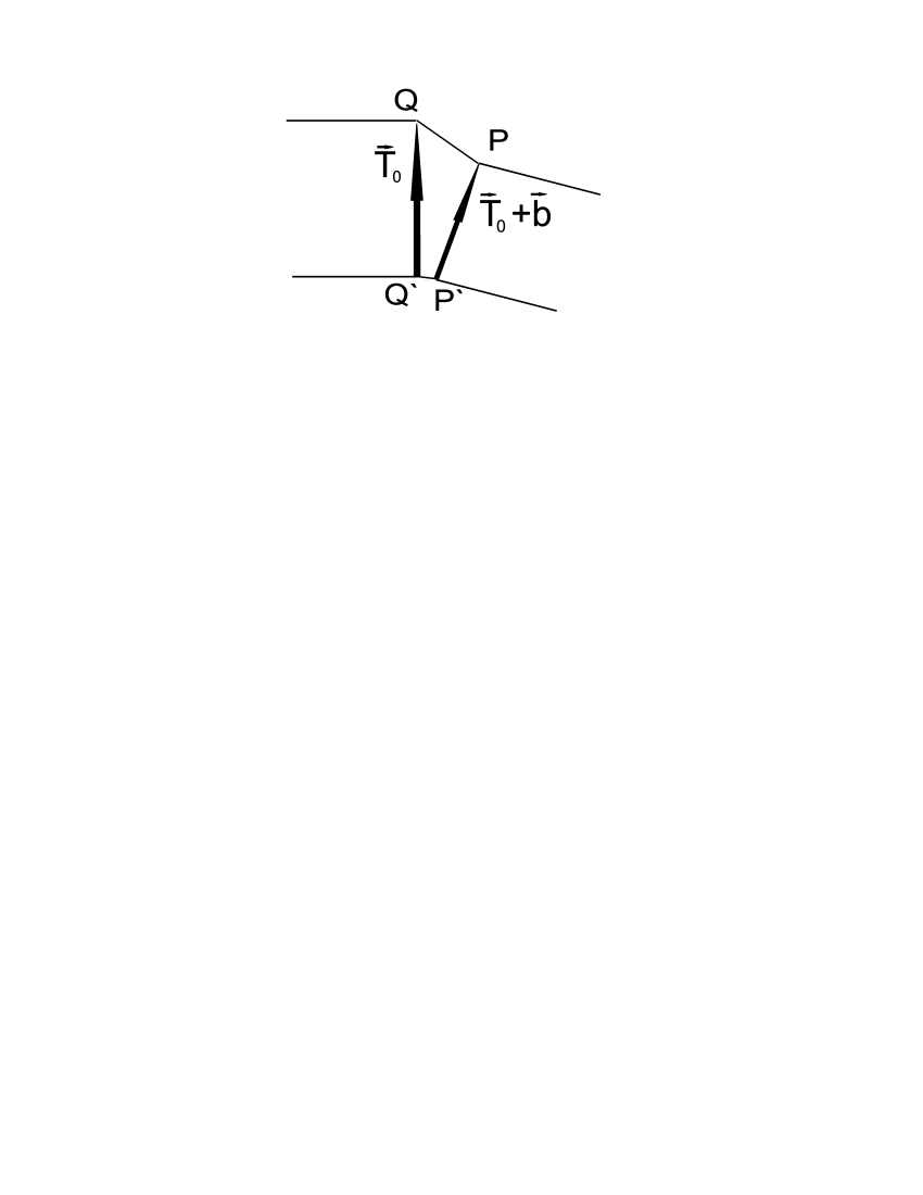
Figure 1: The schematic structure of the nanotube in the defect region. The fivefold is located at the point Q (Q’), and the sevenfold - at the point P (P’). Both the length and the direction of the translational vector $\vec{T}_{0}$ are changed in the presence of the 5-7 disclination dipole.

Generally, the DD with a distortion vector $\vec{b}$ changes both the length and the direction of the translational vector. As a result, on the right side the shape of the tube is also a cylinder with the radius $|\vec{T}_{0}+\vec{b}|/(2\pi)$, displaced by the angle between vectors $\vec{T}_{0}$ and $\vec{T}_{0}+\vec{b}$. In this paper, we consider $b/T_{0}$ as a small parameter. As an example, this could be the vector $\vec{b}(2,1)$ which preserves the metallicity of the tube. Reverting to the shape of the tube we should roll up the development. This resembles the ”cut-and-glue” procedure for a disclination in the nanocone [7]. This procedure determines an explicit relative positions for the cylinders (both the angle and the distance between the axis lines) as a function of $\vec{b}$. For the exact shape of the structure in the junction region, let us construct a phenomenological approximation, which satisfies all the boundary conditions described above.

Let us associate the development with the xy-plane and choose the axis along the tube on the left side as the x-axis. In this case, one has $\vec{T}_{0}(0,T_{0},0)$ and $\vec{T}(\xi)=\vec{T}(T_{x},T_{y},0)$. It is convenient to introduce the new frame with the vector $\vec{n}=(\vec{T}\times\vec{e}_{z})/T$ ($\vec{e}_{i}\,(i=x,y,z)$ are the orthogonal basis vectors) which follows the tube axis (see Fig. 2).

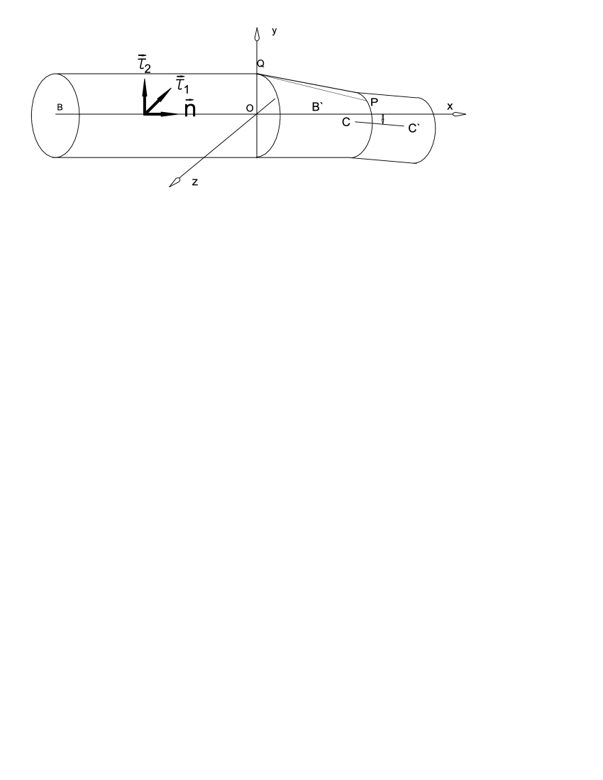
Figure 2: A schematic picture of the nanotube surface. The fivefold is located at the point Q, and the sevenfold - at the point P. The thick tube axis BB’ coincides with the x-axis. The thin tube axis CC’ is shifted due to the disclination dipole QP.

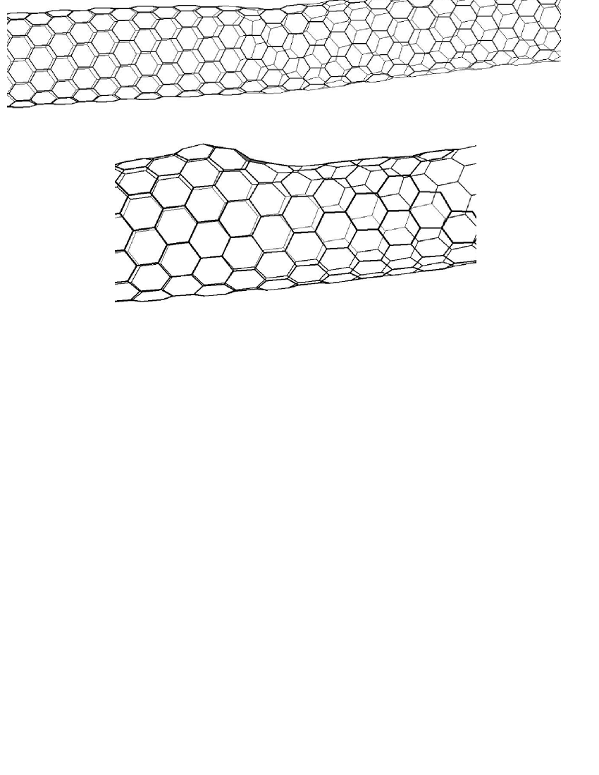
Figure 3: A molecular-dynamics simulation for the shape of the (12,0)-(10,1) junction [9]. Bottom: in the junction region the shifting of the tube axis can be observed.

The orthogonal to $\vec{n}$ vectors are $\vec{\tau}_{1}=-\vec{e}_{z}$ and $\vec{\tau}_{2}=\vec{\tau}_{1}\times\vec{n}=\vec{T}/T$. To take into account the disclination dipole, which is situated at the top of the cylinder, one needs to describe the skewed conical surface between $Q$ and $P$ points. Actually, the DD has two effects: it changes the radius and shifts the surface of the tube in the direction normal to the tube axis. Since the radius $R(\xi)=T(\xi)/(2\pi)$ changes its value on $\Delta R$, the ring will be shifted in the direction of $\vec{\tau}_{2}$ by $\Delta R$, so that we must add the shift $\vec{\tau}_{2}T/(2\pi)$.

Finally, the surface is parametrized as following:

$$\vec{r}=\vec{n}\xi+\vec{\tau}_{2}\frac{T}{2\pi}+\vec{\tau}_{1}\frac{T}{2\pi}\cos\varphi+\vec{\tau}_{2}\frac{T}{2\pi}\sin\varphi,$$ (1)

where $-\infty<\xi<\infty$ and $0\leq\varphi<2\pi$ are the normal and the transversal coordinates, respectively.

The form of the tube with 5-7 rings is supposed to be

$$\vec{r}(\xi\frac{T_{y}}{T}+\frac{T_{x}}{2\pi}(1+\sin\varphi),-\xi\frac{T_{x}}{T}+\frac{T_{y}}{2\pi}(1+\sin\varphi),-\frac{T}{2\pi}\cos\varphi)$$ (2)

where we assume

$$\vec{T}(\xi)=\vec{T}_{0}+\frac{\vec{b}}{2}(\tanh\frac{\xi}{\xi_{0}}+1)$$ (3)

to be the tube translation vector, depending on the coordinate $\xi$, the distortion vector $\vec{b}$ and an effective parameter $\xi_{0}$, which corresponds to the half-width of the surface region curved by the DD. Since the surface of the nanotube has high but finite Young modulus, one can expect that $\xi_{0}$ is of the same order as $R_{0}$. Let us calculate the geometrical properties of the tube in the first order in $\vec{b}$.

The metric tensor is found to be

$$g_{\xi\xi}=1+\xi\frac{(T^{2})^{\prime}}{T^{2}}-2\xi\frac{T^{\prime}}{T}+2\frac{T_{y}T_{x}^{\prime}-T_{x}T_{y}^{\prime}}{2\pi T}(1+\sin\varphi)+{\cal O}(b^{2})=1+\gamma_{\xi\xi},$$

$$g_{\xi\varphi}=\frac{1}{2}\left[\frac{(T^{2})^{\prime}}{4\pi^{2}}-2\xi\frac{T_{y}T_{x}^{\prime}-T_{x}T_{y}^{\prime}}{2\pi T}\right]\cos\varphi+{\cal O}(b^{2})=\gamma_{\xi\varphi},$$

$$g_{\varphi\varphi}=R_{0}^{2}+\frac{\vec{T}_{0}\cdot\vec{b}}{4\pi^{2}}(\tanh\frac{\xi}{\xi_{0}}+1)+{\cal O}(b^{2})=R_{0}^{2}+\gamma_{\varphi\varphi},$$ (4)

and

$$g^{\xi\xi}=1-\gamma_{\xi\xi},\;g^{\xi\varphi}=-\frac{\gamma_{\xi\varphi}}{R_{0}^{2}},\;g^{\varphi\varphi}=\frac{1}{R_{0}^{2}}-\frac{\gamma_{\varphi\varphi}}{R_{0}^{4}}.$$ (5)

The metrical connection

$$\Gamma^{k}_{\mu\lambda}=\frac{1}{2}g^{kl}(\partial_{\mu}g_{l\lambda}+\partial_{\lambda}g_{\mu l}-\partial_{l}g_{\mu\lambda})$$ (6)

is found to be

$$\Gamma^{\xi}_{\xi\xi}=\partial_{\xi}\gamma_{\xi\xi}/2;\;\Gamma^{\xi}_{\xi\varphi}=\Gamma^{\xi}_{\varphi\xi}=\partial_{\varphi}\gamma_{\xi\xi}/2;$$

$$\Gamma^{\xi}_{\varphi\varphi}=\partial_{\varphi}\gamma_{\xi\varphi}-\partial_{\xi}\gamma_{\varphi\varphi}/2;$$

$$\Gamma^{\varphi}_{\xi\xi}=\partial_{\xi}\gamma_{\xi\varphi}/R_{0}^{2}-\partial_{\varphi}\gamma_{\xi\xi}/(2R_{0}^{2});$$

$$\Gamma^{\varphi}_{\xi\varphi}=\Gamma^{\varphi}_{\varphi\xi}=\partial_{\xi}\gamma_{\varphi\varphi}/(2R_{0}^{2}),$$ (7)

and $\Gamma^{\varphi}_{\varphi\varphi}=0$. Tetradic coefficients $e^{i}_{\;\mu}$, which are determined by the equation

$$g_{\mu\nu}=e^{i}_{\;\mu}e^{k}_{\;\nu}\delta_{ik},$$ (8)

are chosen to be

$$e^{1}_{\;\xi}=1+\frac{\gamma_{\xi\xi}}{2};\,e^{1}_{\;\varphi}=\gamma_{\xi\varphi};\,e^{2}_{\;\xi}=0;\,e^{2}_{\;\varphi}=R_{0}+\frac{\gamma_{\varphi\varphi}}{2R_{0}}$$ (9)

and

$$e_{1}^{\;\xi}=1-\frac{\gamma_{\xi\xi}}{2};\,e_{1}^{\;\varphi}=0;$$

$$e_{2}^{\;\xi}=-\frac{\gamma_{\xi\varphi}}{R_{0}};\;e_{2}^{\;\varphi}=\frac{1}{R_{0}}-\frac{\gamma_{\varphi\varphi}}{2R_{0}^{3}}.$$ (10)

The spin connection coefficients

$$(\omega_{\mu})^{ab}=e^{a}_{\;\nu}D_{\mu}e^{b\nu},$$

where $D_{\mu}:=\partial_{\mu}+\Gamma_{\mu}$ is a covariant derivative, reads

$$\omega_{\xi}^{\;12}=-\frac{\partial_{\xi}\gamma_{\xi\varphi}}{R_{0}}+\frac{\partial_{\varphi}\gamma_{\xi\xi}}{2R_{0}}=\left[-\frac{(T^{2})^{\prime\prime}}{8\pi^{2}R_{0}}+\xi\frac{T_{y}T_{x}^{\prime\prime}-T_{x}T_{y}^{\prime\prime}}{4\pi^{2}R_{0}^{2}}\right]\cos\varphi;$$

$$\omega_{\varphi}^{\;12}=-\frac{\partial_{\xi}\gamma_{\varphi\varphi}}{2R_{0}}=-\frac{(T^{2})^{\prime}}{8\pi^{2}R_{0}};\;\omega_{\mu}^{\;21}=-\omega_{\mu}^{\;12}.$$ (11)

2 CONDUCTIVITY AND THE FANO FACTOR

From now on we set $E_{F}=0,\,V_{F}=\hbar=1$. The Dirac equation on the curved surface is defined as

$$-i\sigma_{i}e_{i}^{\;\mu}(\nabla_{\mu}-iA_{\mu})\psi=E\psi,$$ (12)

with $\sigma_{i}$ being the Pauli matrices ($i={1,2}$), $\psi$ is a 2-component spinor wavefunction, and $A_{\mu}\;(\mu={\xi,\,\varphi})$ being the DD field. The derivative includes a spin connection term $\Omega_{\mu}$ and it is written as

$$\nabla_{\mu}=\partial_{\mu}+\Omega_{\mu},\;\Omega_{\mu}=\frac{1}{8}\omega_{\mu}^{\;ab}[\sigma_{a},\sigma_{b}].$$

In the linear in $\vec{b}$ approximation the Dirac equation takes the form

$$-i\sigma_{1}e^{1\xi}(\nabla_{\xi}-iA_{\xi})\psi-i\sigma_{2}(e^{2\xi}\partial_{\xi}+e^{2\varphi}(\nabla_{\varphi}-iA_{\varphi}))\psi=E\psi,$$ (13)

with the covariant derivatives written as

$$\nabla_{\varphi}=\partial_{\varphi}-\frac{(T^{2})^{\prime}}{16\pi^{2}R_{0}}\sigma_{3};$$

$$\nabla_{\xi}=\partial_{\xi}+[-\frac{(T^{2})^{\prime\prime}}{8\pi^{2}R_{0}}+\xi\frac{T_{y}T_{x}^{\prime\prime}-T_{x}T_{y}^{\prime\prime}}{4\pi^{2}R_{0}^{2}}]\frac{\sigma_{3}}{2}\cos\varphi.$$ (14)

Substituting (2) into (13) we find both the undisturbed Dirac operator $\hat{\cal D}_{0}$

$$\hat{\cal D}_{0}=-i\sigma_{1}\partial_{\xi}-i\frac{\sigma_{2}}{R_{0}}\partial_{\varphi},$$ (15)

and the perturbation operator $\hat{\cal V}$

$$\hat{\cal V}=i\sigma_{1}\frac{\gamma_{\xi\xi}}{2}\partial_{\xi}-i\sigma_{1}\Omega_{\xi}-\sigma_{1}A_{\xi}+i\sigma_{2}\frac{\gamma_{\xi\varphi}}{R_{0}}\partial_{\xi}-i\frac{\sigma_{2}}{R_{0}}\Omega_{\varphi}-\frac{\sigma_{2}}{R_{0}}A_{\varphi}+i\sigma_{2}\frac{\gamma_{\varphi\varphi}}{2R_{0}^{3}}\partial_{\varphi}.$$ (16)

It should be mentioned that the perturbation (16) includes the last term, which is not localized (differs from zero value at $\xi\rightarrow\infty$). Therefore an analysis of (15) and (16) differs from a typical scattering problem. To simplify the problem, let us restrict our consideration to the lowest term with the zero angular momentum, that is only a plain wave $\psi(\xi,\varphi)=(1,\pm 1)^{T}e^{ik\xi}$ is considered. In this case in (15) and (16) only the zero-momentum terms should be taken into account in the Fourier series for the angle-dependent part of the wavefunction.

As a result, instead of (15) and (16) there should apper an equation for the zero-momentum part of the wavefunction with the Dirac hamiltonian $\hat{\cal D}_{0}=-i\sigma_{1}\partial_{\xi}$ and the perturbation

$$\hat{\cal V}=i\sigma_{1}\frac{(\vec{b}\times\vec{T}_{0})_{z}}{8\pi^{2}R_{0}\xi_{0}\cosh^{2}(\xi/\xi_{0})}\partial_{\xi}-\sigma_{1}<A_{\xi}>_{\varphi}-\sigma_{1}\frac{\vec{b}\cdot\vec{T}_{0}}{16\pi^{2}R_{0}^{2}\xi_{0}\cosh^{2}(\xi/\xi_{0})}-\frac{\sigma_{2}}{R_{0}}<A_{\varphi}>_{\varphi}.$$ (17)

Here $<>_{\varphi}$ denotes the averaging over $\varphi$ and $(\vec{b}\times\vec{T}_{0})_{z}=b_{x}T_{0y}-T_{0x}b_{y}$. Now the perturbation (17) is localized near $\xi=0$ with a half-width $\xi_{0}$. In order to remove the differentiation in (17) one can multiply the operator $\hat{\cal D}_{0}+\hat{\cal V}$ by

$$\left(1+\frac{(\vec{b}\times\vec{T}_{0})_{z}}{8\pi^{2}R_{0}\xi_{0}\cosh^{2}(\xi/\xi_{0})}\right).$$

In this case, the additional potential

$$IE(\vec{b}\times\vec{T}_{0})_{z}/(8\pi^{2}R_{0}\xi_{0}\cosh^{2}(\xi/\xi_{0}))$$

appears, where $I$ is a unit matrix.

The field $\vec{A}$ describes the DD-induced valley mixing. It may be written as $A_{j}=\mu\epsilon_{jk}\partial_{k}G$ where $j,k=\xi,\,\varphi$, $\mu$ is an effective ”charge” of each disclination, $G$ is a dipole potential, which satisfies the equation

$$\nabla^{2}G(\xi,\varphi)=\frac{2\pi}{R}[d_{\xi}\delta^{\prime}(\xi)\delta(\varphi)+d_{\varphi}\delta(\xi)\delta^{\prime}(\varphi)/R_{0}],$$

$\nabla^{2}=\partial^{2}_{\xi}+\partial^{2}_{\varphi}/R_{0}^{2}$, $\epsilon_{jk}$ is a unit antisymmetric tensor, $\delta(x)$ and $\delta^{\prime}(x)$ are the Dirac delta function and it’s derivative, and $\vec{d}$ is a vector connecting five- and sevenfold (it has the same order as $\vec{b}$ [11]). Explicitly, one can find $G$ in a form

$$G(\xi,\varphi)=-\frac{2\pi^{2}}{R_{0}}\sum_{n}[d_{\xi}\mathop{\mathrm{sign}}\nolimits(\xi)+\frac{id_{\varphi}}{R}\mathop{\mathrm{sign}}\nolimits(n)]e^{in\varphi}e^{-|n\xi|/R_{0}}.$$ (18)

For the zero momentum $n=0$, the field $\vec{A}$ has the form

$$A_{\xi}=0,\;A_{\varphi}=\frac{4\pi^{2}\mu b_{\xi}}{R_{0}}\delta(\xi),$$ (19)

where $\delta(\xi)$ is a Dirac delta function. Finally, the perturbation operator looks as following:

$$\hat{\cal V}=-I\frac{(\vec{b}\times\vec{T}_{0})_{z}\,E}{8\pi^{2}R_{0}\xi_{0}\cosh^{2}(\xi/\xi_{0})}-\sigma_{1}\frac{\vec{b}\cdot\vec{T}_{0}}{16\pi^{2}R_{0}^{2}\xi_{0}\cosh^{2}(\xi/\xi_{0})}-\sigma_{2}\frac{4\pi^{2}\mu d_{\xi}}{R_{0}^{2}}\delta(\xi).$$ (20)

Notice that the last term in (20) corresponds to the $\xi$-dependent mass term $\sigma_{2}m(\xi)$ in the Dirac equation. Let us calculate the transfer matrix and the conductance according to the method described in [12] and [13]. To transform the initial Dirac equation to the diagonal form, the unitary rotation is performed: $\psi\rightarrow{\cal{L}}\psi,\,\hat{\cal V}\rightarrow{\cal{L}}\hat{\cal V}{\cal{L}^{\dagger}},\,\sigma_{i}\rightarrow{\cal{L}}\sigma_{i}{\cal{L}^{\dagger}},\;{\cal{L}}=(\sigma_{1}+\sigma_{3})/\sqrt{2}.$ For zero angular momentum, the equation for the transfer matrix reads

$${\cal T}(\frac{L}{2},-\frac{L}{2})={\cal T}^{(0)}(\frac{L}{2},-\frac{L}{2})-i\int_{-\frac{L}{2}}^{\frac{L}{2}}dx{\cal T}^{(0)}(\frac{L}{2},x)\sigma_{3}\hat{\cal V}(x){\cal T}(x,-\frac{L}{2}),$$ (21)

where ${\cal T}^{(0)}(x_{2},x_{1})=\exp(i\sigma_{3}E(x_{2}-x_{1}))$ and $L$ is the length of the tube. The perturbation (20) takes the form

$$\sigma_{3}\hat{\cal{V}}=-\sigma_{3}\frac{(\vec{b}\times\vec{T}_{0})_{z}\,E}{8\pi^{2}R_{0}\xi_{0}\cosh^{2}(\xi/\xi_{0})}+I\frac{\mu b_{y}}{\xi^{2}+\pi^{2}R_{0}^{2}}-$$

$$-I\frac{\vec{b}\cdot\vec{T}_{0}}{16\pi^{2}R_{0}^{2}\xi_{0}\cosh^{2}(\xi/\xi_{0})}-i\sigma_{1}\frac{4\pi^{2}\mu d_{\xi}}{R_{0}^{2}}\delta(\xi).$$ (22)

We assume that $L$ is much larger than $\xi_{0}$. In the linear in $\vec{b}$ approximation one can replace ${\cal T}$ by ${\cal T}^{(0)}$ in the integral in (21). In our consideration, the direct intervalley scattering is not taken into account. Thus one can consider two inequivalent $K$-points (valleys) as two different channels coupled by the non-Abelian field. Therefore, one should perform a replacement $\mu\rightarrow\mu\tau_{2}$ with $\mu=1/4$ and $\tau_{2}$ being the Pauli matrix in the channel space representing the mixing of sublattices due to pentagonal and hexagonal defects (see [7] for detail). By substituting (2) into (21) and taking the limits of integration to be infinity, one obtains the transfer matrix in the form

$${\cal T}=\exp(i\sigma_{3}EL)+i[\frac{\vec{b}\cdot\vec{T}_{0}}{8\pi^{2}R_{0}^{2}}+\sigma_{3}\frac{(\vec{b}\times\vec{T}_{0})_{z}E}{4\pi^{2}R_{0}}]\exp(i\sigma_{3}EL)+\mu d_{\xi}\sigma_{1}\tau_{2}\frac{4\pi^{2}}{R_{0}^{2}}.$$ (23)

The scattering matrix $(t^{{\dagger}})^{-1}$ is defined by the upper-left element of the transfer matrix, so that the last term in (23) is neglected. The conductance is defined as $G=(4e^{2}/h)Tr[t^{\dagger}t]$, where the trace is taken over the channel space. It takes the form

$$G=\frac{4e^{2}}{h}[1-\left(\frac{\vec{b}\cdot\vec{T}_{0}}{2T_{0}^{2}}+\frac{(\vec{b}\times\vec{T}_{0})_{z}\epsilon}{T_{0}^{2}}\right)^{2}],$$ (24)

where $\epsilon=ER_{0}$ is a dimensionless energy (in the absolute units of $hV_{F}/R_{0}$). Correspondingly, the Fano factor $F=1-Tr[(t^{\dagger}t)^{2}]/Tr[t^{\dagger}t]$ reads

$$F={\left(\frac{\vec{b}\cdot\vec{T}_{0}}{2T_{0}^{2}}+\frac{(\vec{b}\times\vec{T}_{0})_{z}\epsilon}{T_{0}^{2}}\right)}^{2}.$$ (25)

One can see that the mass-type term (the DD term) does not influence both the conductance and the Fano factor since only linear terms in $\vec{b}$ are taken into account (the mass is expected to be the second-order term). Depending on the angle between $\vec{T}_{0}$ and $\vec{T}_{0}+\vec{b}$, two types of energy-dependent behaviour appear. For the angle less than $\pi/2$, both the scalar and ”vector” products in (24) and (25) are of the same sign. In this case, the linear in energy term in (24) leads to a decrease of the conductance with increasing energy (and vice versa), see Fig.4 (black line). This case corresponds to slightly curved tubular structures. For the second type of behaviour, when the angle is greater than $\pi/2$ the increasing of conductance is expected with energy increasing. A special case is presented on Fig.4 (gray line), with $\vec{T}_{0}$ and $\vec{b}$ orthogonal, where a transmission coefficient is equal to unity at the Fermi energy $\epsilon=0$. However, in this case the higher-order perturbation terms should be included.

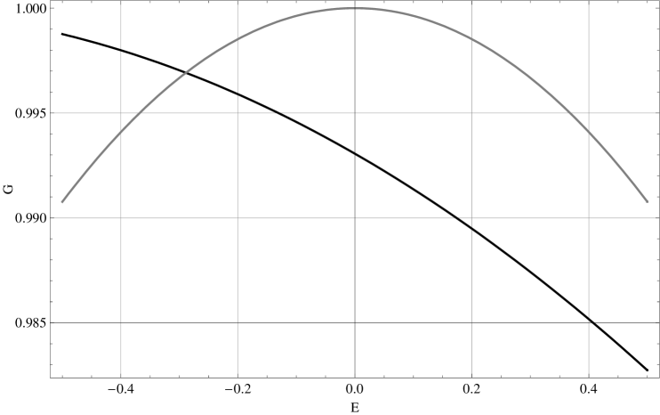
Figure 4: Conductance $G$, in the units of $h/(4e^{2})$, depending on the energy $E$ in the units of $hV_{F}/R_{0}$, through the metallic junction (9,0) - (11,1) tubes (black line) and (9,0) - (10,2) (gray line).

CONCLUSION

In this paper, we have investigated the electronic transport properties of metallic nanotubes with the disclination dipole defect. The case of disclination dipoles preserving the chirality (metallic character of the tube) was considered. This assumption simplifies the problem under consideration and allows us to construct a self-consistent expansion scheme for the effective Dirac equation. The perturbation includes both the curvature term, which appear as the Gaussian-like smooth localized potential, and the DD-induced term. The standard transfer-matrix approach is used to calculate the conductance and the Fano factor of the structure.

As the marked effect of the curvature, the energy-dependent term in both the conductance and the Fano factor appears. It should be stressed that the tube length $L$ and the effective half-width $\xi_{0}$ do not enter the final results. This differs from the case of ballistic transport in graphene with various types of disorder studied in [13], where both the conductance and the Fano factor were found to depend on the sample length (or, more precisely, on $EL$).

Notice that in [14], [8] a similar model for two metallic nanotubes of different radiuses connected by the conical interface was constructed. The transmission probability was found to decrease when the difference of tube radiuses (which is determined by $b_{y}$ in our paper) increases, which is in agreement with the $~{}1-\alpha b^{2}$ behaviour in (24). The origin of this behaviour within our model is purely geometrical, while in  [14] the boundary conditions for the wavefunction incorporates both the ”geometrical” factor and the mixing of the K-points within the junction. As for the energy dependence, in [8] the conductance was found to decrease with energy increasing for (17,17)-(18,21) junction, and subsequently the increasing of conductance was found for (23,8)-(16,22) junction. This fact is in general agreement with (24), where the character of energy behaviour depends on the angle between translational (chiral) vector and the distortion vector (the difference of chiral vectors). At higher energies close to band edges, a more complex behaviour of conductance was predicted, which is absent in our model. The source of this difference is twofold. First, instead of the boundary conditions on the tube-cone interface in [14] and[8] we consider the model with smooth shape of the structure, so that the resonant behaviour of wavefunction in the junction region does not appear in our case. Second, for simplicity terms with higher momenta were not included in our model and, as a result, localized and resonant states are absent even at low energies. A self-consistent inclusion of higher momenta in our approach is an important open problem.

The disclination dipole is taken into account via the non-Abelian field, which leads to the mixing of valleys in the low-energy behaviour. The influence of this field was found to be negligible within the perturbational approach compared to the influence of curvature, in contrast with the case of ordinary vortex topological field sources [15]. A dominating process of valley-mixing was taken into account (as it is estimated for the scattering in carbon nanocones [7]) instead of the real intervalley scattering, which is expected to be omitted. This results in the correction of the conductance and the Fano factor in the highest order in $\vec{b}$ to have the same form as for the single-channel approximation. One should also note, that within our model the chirality-dependence of the potential was neglected, because both the left and right ends of the tube with the disclination dipole are of the metallic-type (despite the fact that the radius and exact chirality indices are different). In the general case, one should expect the influence of the defect on transport properties to be sensitive on the tube chiralities, as it was observed in [3]. Another important question is the finiteness of the free electron path in the real tube. As it is easy to see, the phenomenological localization length of the curved area does not influence the transport properties within the constructed approximation. Due to this fact, an effective long-range influence of topological defects could possibly lead to the non-trivial interplay with the mean free path length in the tubes with disclination dipoles.

We would like to thank O.E.Gluhova for the results of molecular-dynamics calculations.

This work has been supported by the Russian Foundation for Basic Research under grant No. 08-02-01027.

References

- [1] Y.Ma et al. Magnetic properties of vacancies in graphene and single-walled carbon nanotubes// New J. Phys. 2004. V. 6. P. 68.
- [2] P.O.Lethinen et al. Structure and magnetic properties of adatoms on carbon nanotubes// Phys. Rev. B. 2004. V. 69. P. 155422.
- [3] T.Nakanishi, M.Igami and T.Ando. Conductance Quantization in the Presence of Huge and Short-Range Potential in Carbon Nanotubes// Physica E. 2000. V. 6. P. 872.
- [4] L. Chico et al. Pure Carbon Nanoscale Devices: Nanotube Heterojunctions// Phys. Rev. Lett. 1996. V. 76. P. 971.
- [5] N.Chandra, S. Namilae, and C. Shet. Local elastic properties of carbon nanotubes in the presence of Stone-Wales defects// Physical Review B. 2004. V. 69. P. 094101.
- [6] M.A.H.Vozmediano, M.I.Katznelson, and F.Guinea. Gauge fields in graphene// arXiv:1003.5179. 2010.
- [7] P. Lammert and V. Crespi. Graphene cones: Classification by fictitious flux and electronic properties// Phys.Rev.B. 2004. V. 69. P. 035406.
- [8] R.Tamura and M.Tsukada. Relation between transmission rates and the wave functions in carbon nanotube junctions // Phys.Rev.B. 2000. V. 61. P. 8548.
- [9] O.E.Gluxova. Private message.
- [10] C.L.Kane and E.J.Mele. Size, Shape, and Low Energy Electronic Structure of Carbon Nanotubes// Phys. Rev. Lett. 1997. V. 78. P. 1932.
- [11] For the planar case, ; see O.V.Yazyev and S.G.Louie. arXiv:1004.203. 2010.
- [12] M. Titov. Impurity-assisted tunneling in graphene// Europhys. Lett. 2007. V. 79. P. 17004.
- [13] A. Schuessler et al. Analytic theory of ballistic transport in disordered graphene// Phys. Rev. B. 2009. V. 79. P. 075405.
- [14] H.Matsumura and T.Ando. Topological Effects on Conductance of Nanotubes// Mol. Cryst. Liq. Cryst. 2000. V. 340. P. 725.
- [15] D. V. Kolesnikov and V. A. Osipov. The continuum gauge field-theory model for low-energy electronic states of icosahedral fullerenes// Europhys. J. B. 2006. V. 49. P. 465.