Correlators of supersymmetric Wilson loops at weak and strong coupling

Abstract:

We continue our study of the correlators of a recently discovered family of BPS Wilson loops in ${\cal N}=4$ supersymmetric $U(N)$ Yang-Mills theory. We perform explicit computations at weak coupling by means of analytical and numerical methods finding agreement with the exact formula derived from localization. In particular we check the localization prediction at order $g^{6}$ for different BPS “latitude” configurations, the ${\cal N}=4$ perturbative expansion reproducing the expected results within a relative error of $10^{-4}$. On the strong coupling side we present a supergravity evaluation of the 1/8 BPS correlator in the limit of large separation, taking into account the exchange of all relevant modes between the string worldsheets. While reproducing the correct geometrical dependence, we find that the associated coefficient does not match the localization result.

1 Introduction

The maximally supersymmetric Yang-Mills theory provides the simplest dynamics among the four-dimensional gauge theories and has represented an important and interesting laboratory from the theoretical perspective. Not only is it believed that the theory has an exact dual description, the type IIB ten-dimensional string theory in the AdS${}_{5}\times S^{5}$ background [1], but new fascinating connections have appeared throughout the years. The integrable structures underlying the spectrum of the anomalous dimensions [2, 3], the exact exponentiation properties observed in scattering amplitudes [4] and the possible connection with the geometric Langlands program [5] are just a few examples of the richness still hidden in ${\cal N}$ = 4 SYM.

Remarkably exact results exist also for Wilson loops, which in ${\cal N}$ = 4 theory can be generalized to preserve some amount of superconformal symmetry. The simplest operator of this kind is a circular Wilson loop which couples to one of the six adjoint scalar fields of the theory: it is called the 1/2 BPS Wilson loop because it preserves one half of the 32 superconformal symmetries. It was conjectured [6, 7] that the expectation value of such an operator can be computed in the Gaussian matrix model. The conjecture was supported by an explicit two-loop perturbative computation, while from the dual string theory point of view, in a suitable limit of large $N$ and large ’t Hooft constant $\lambda=g^{2}_{YM}N$, the Gaussian matrix model nicely agrees with the solution to the minimal area problem [8, 9]. More generally other kinds of Wilson loops, which preserve various amounts of supersymmetry have been constructed and studied. In particular a family of 1/16 BPS Wilson loops of arbitrary shape on a three-sphere $S^{3}$, embedded in the Euclidean four dimensional space-time, were presented in [10, 11] . Restricting the contour of the loops to the equator one gets 1/8 BPS Wilson loops and a conjecture in this case has been proposed: the expectation value of such Wilson loops is captured by the zero-instanton sector of the ordinary bosonic two-dimensional Yang-Mills living on the $S^{2}$. The coupling constant of the 2d Yang-Mills theory is related to the coupling constant of the ${\cal N}$=4 SYM as $g^{2}_{2d}=-g^{2}_{4d}/(2\pi r^{2})$, where $r$ is the radius of the $S^{2}$. The loops are still computed by a Gaussian matrix model, the circular Wilson loop being a particular case of this general family.

This conjecture was further supported at order $g^{4}$ in [12, 13] for the expectation value of a single Wilson loop operator of arbitrary shape on $S^{2}$, and further extended at the level of BPS correlators of Wilson loops [14, 15], where the multi-matrix model describing the correlators in the zero-instanton sector of YM₂ has been derived. Non-trivial consistency checks and explicit computations supporting the conjecture for correlators have also been performed [15]. The conjecture has been recently extended to include ’t Hooft loops and S-duality, taking into account non-trivial instanton sectors [16].

The emergence of a two-dimensional theory underlying the dynamics of some BPS sectors of ${\cal N}$=4 SYM can be understood from the localization of the four-dimensional path integral to particular supersymmetric configurations, as recently shown by [17, 18]. The moduli space of solutions to the supersymmetry equations is parameterized by two-dimensional data and the effective action governing the relevant dynamics is the semi-topological Hitchin/Higgs-Yang-Mills theory: the computation of regular 1/8 BPS observables can be mapped there and reduces to usual YM₂ on $S^{2}$.

The localization of the path-integral in four-dimensional supersymmetric gauge theories is not a novelty: the exact computation of the prepotential in ${\cal N}=2$ SYM has been derived in [19] through this kind of procedure, summing up all instanton contributions. Actually the result concerning the 1/2 BPS Wilson loop can be extended to ${\cal N}=2^{*}$ SYM theories, taking also into account the contribution of instantons (which decouple in the ${\cal N}=4$ case). Quite recently, from the exact expression of the partition function derived from the localization approach of [17], a rather general class of ${\cal N}=2$ superconformal gauge theories introduced in [20] has been shown to be described by two-dimensional Liouville theory [21].

It appears therefore important to test the results expected from path-integral localization through the familiar perturbative QFT methods and the AdS/CFT correspondence, even in the simplest case of ${\cal N}=4$ where some checks are still missing. In particular the two-dimensional gauge theory should compute not only the expectation value of a single 1/8 BPS Wilson operator but even correlators of loops preserving the same amount of supersymmetry. A first step in this direction was taken in [13], where an apparent disagreement was observed in the limit of coincident loops. Later the relevant matrix-model result was shown to be consistent with the supergravity picture [14]. In [15] we started a systematic approach to the computation of the correlator of two “latitude” BPS Wilson loops, at weak coupling by perturbation theory and at the strong coupling through AdS/CFT correspondence. We checked the formula derived from the zero-instanton sector of YM₂ at order ${\cal O}(g^{4})$ and we showed that, in the limit where one of the loops shrinks to a point, logarithmic corrections in the shrinking radius are absent at ${\cal O}(g^{6})$. This last result strongly supported the validity of the general expression and suggested the existence of a peculiar protected local operator arising in the OPE of the Wilson loop (see also [22] for a related investigation). Using the string dual of the ${\cal N}=4$ SYM correlator in the limit of large separation, we also presented some preliminary evidence for the agreement at strong coupling.

In this paper we continue our study of the two-latitude correlator, extending our previous investigations. First of all we present strong evidence that the weak coupling perturbative computation agrees with the matrix model expression. We evaluate numerically the expectation value of correlators at order $g^{6}$ for two particular configurations: a symmetric one in which the loops are two latitudes at polar angle $\theta=\delta$ and $\theta=\pi-\delta$ (1/4 BPS system) and the other with a loop fixed on the equator $\theta=\pi/2$ and the second at generic angle $\theta=\delta$ (1/8 BPS system). No particular limit has been considered and the agreement is quite good over the whole range of our study, including angles $\delta$ between $0.7$ and $\pi/2$. The relative error between the YM₂ prediction and the ${\cal N}=4$ SYM calculation is of the order of $10^{-5}$. For values of $\delta$ less than 0.7 the requirement on the precision of the calculation of certain integrals becomes prohibitive. Generically, the errors involved grow in the opposite (coincident) limit of $\delta=\pi/2$, however we find that they are manageable even when $\delta$ is very close to $\pi/2$. The supergravity calculation is also tackled and should reproduce the strong coupling result, at large $N$, of the exact localization answer: unfortunately we were not able to find such agreement. We compute the exchange of supergravity modes between the widely separated worldsheets describing the Wilson loops at strong coupling. We identify all modes contributing to the correlator at leading order in the large separation limit. While the sum of these exchanges produces a qualitative agreement with the matrix model, we observe a deviation in the numerical coefficient. We comment on this puzzle and will leave its resolution to future investigations.

The plan of the paper is the following: in Section 2 we briefly recall the structure of the BPS Wilson loops, their expectation values and correlators according to the localization formula and discuss our previous results. In Section 3 we present our numerical computation in detail, explaining our procedure and critically examining the numerical agreement. In Section 4 the strong coupling computation is performed in detail using the familiar methods of AdS/CFT, and the origin of the mismatch is discussed. In Section 5 we draw our conclusions and discuss future directions of research.

2 The supersymmetric Wilson loops and their correlators

We start by considering the family of BPS Wilson loops that has been introduced in [11]: a simple way to understand this construction is to observe that it is possible to pack three of the six real scalars present in ${\cal N}=4$ SYM into a self-dual tensor

$$\Phi_{\mu\nu}=\sigma^{i}_{\mu\nu}M^{i}{}_{I}\Phi^{I}\,,$$ (1)

and to use the modified connection

$$A_{\mu}\to A_{\mu}+i\Phi_{\mu\nu}x^{\nu}\,$$ (2)

in the Wilson loop. The crucial elements in this definition are the tensors $\sigma^{i}_{\mu\nu}$: they can be defined by the decomposition of the Lorentz generators in the anti-chiral spinor representation ($\gamma_{\mu\nu}$) into Pauli matrices $\tau_{i}$

$$\frac{1}{2}(1-\gamma^{5})\gamma_{\mu\nu}=i\sigma^{i}_{\mu\nu}\tau_{i}\,,$$ (3)

where the projector on the anti-chiral representation is included ($\gamma^{5}=-\gamma^{1}\gamma^{2}\gamma^{3}\gamma^{4}$). The matrix $M^{i}{}_{I}$ appearing in (1) is $3\times 6$ dimensional and is norm preserving, i.e. $MM^{\top}$ is the $3\times 3$ unit matrix (an explicit choice of $M$ is $M^{1}{}_{1}=M^{2}{}_{2}=M^{3}{}_{3}=1$ and all other entries zero).

More geometrically, the tensors $\sigma^{i}_{\mu\nu}$ are related to invariant one-forms on $S^{3}$

$$\sigma_{1}^{R,L} =2\left[\pm(x^{2}dx^{3}-x^{3}dx^{2})+(x^{4}dx^{1}-x^{1}dx^{4})\right]$$ (4)

$$\sigma_{2}^{R,L} =2\left[\pm(x^{3}dx^{1}-x^{1}dx^{3})+(x^{4}dx^{2}-x^{2}dx^{4})\right]$$

$$\sigma_{3}^{R,L} =2\left[\pm(x^{1}dx^{2}-x^{2}dx^{1})+(x^{4}dx^{3}-x^{3}dx^{4})\right],$$

where $\sigma_{i}^{R}$ are the right (or left-invariant) one-forms and $\sigma_{i}^{L}$ are the left (or right-invariant) one-forms: explicitly

$$\sigma_{i}^{R}=2\sigma^{i}_{\mu\nu}x^{\mu}dx^{\nu}\,.$$ (5)

The BPS Wilson loops can then be written in terms of the modified connection $A_{\mu}+i\Phi_{\mu\nu}x^{\nu}$ as

$$W=\frac{1}{N}\,\text{Tr}\,{\cal P}\exp\oint dx^{\mu}\left(iA_{\mu}-\sigma^{i}_{\mu\nu}x^{\nu}M^{i}{}_{I}\Phi^{I}\right).$$ (6)

Actually the operator (6) is supersymmetric only when the loop is restricted to a three dimensional sphere. This sphere can be taken to be embedded in $\mathbb{R}^{4}$, or as a fixed-time slice of $S^{3}\times\mathbb{R}$. The authors of [11] have shown that requiring that the supersymmetry variation of these loops vanishes for arbitrary curves on $S^{3}$ leads to the two equations

$$\gamma_{\mu\nu}\epsilon_{1}+i\sigma^{i}_{\mu\nu}\rho^{i}\gamma^{5}\epsilon_{0} =0\,,$$ (7)

$$\gamma_{\mu\nu}\epsilon_{0}+i\sigma^{i}_{\mu\nu}\rho^{i}\gamma^{5}\epsilon_{1} =0\,,$$

that can be solved consistently: for a generic curve on $S^{3}$ the Wilson loop preserves $1/16$ of the original supersymmetries. We remark that this construction needs the introduction of a length-scale, as seen by the fact that the tensor (1) has mass dimension one instead of two: we will fix the scale to be the radius $r$ of $S^{3}$.

The situation becomes more interesting for special curves, when there are extra relations between the coordinates and their derivatives: in this case there will be more solutions of (7) and the Wilson loops will preserve more supersymmetry. A particularly interesting case is when the loop lies entirely on a $S^{2}$: it is possible to show that these operators are generically 1/8 BPS and Wilson loops lying on the same two-sphere enjoy common supersymmetries. Inspired by the explicit evaluation of the first non-trivial perturbative contribution the authors of [11] conjectured that the 1/8 BPS Wilson loops constructed on $S^{2}$ can be exactly calculated, claiming the equivalence with the computation of Wilson loops in ordinary YM₂ on the sphere, in the zero-instanton sector [23]. Yang-Mills theory on a Riemann surface is completely solvable [24] and the exact expression for the Wilson loop is also available [25]: the restriction of the full answer to the zero-instanton sector follows from rewriting the exact solution as an instanton expansion [26]. Based on this relation, the following exact formula for the quantum expectation value of the 1/8 BPS Wilson operator

$$\langle W\rangle=\frac{1}{N}L_{N-1}^{1}\left(-g_{4d}^{2}\,\frac{A_{1}A_{2}}{A^{2}}\right)\exp\left[\frac{g_{4d}^{2}}{2}\,\frac{A_{1}A_{2}}{A^{2}}\right]\,,$$ (8)

was proposed in [11], where $L_{N-1}^{1}(x)$ is a Laguerre polynomial, $A$ is the area of the sphere and $A_{1,2}$ are the areas enclosed by the loop. The result follows by identifying the two-dimensional coupling constant $g^{2}_{2d}$ with the four-dimensional one through $g^{2}_{2d}=-g_{4d}^{2}/A$ and is equal to the expectation value of the circular Wilson loop, which is computed in a gaussian Hermitian matrix model [6, 7],

$$\langle{W_{C}}\rangle=\left\langle{{1\over N}\text{Tr}\exp(M)}\right\rangle={1\over Z}\int{\cal D}M{1\over N}\text{Tr}\Bigl{[}\exp(M)\Bigr{]}\exp\left(-{2\over g_{4d}^{2}}\text{Tr}M^{2}\right)\,,$$ (9)

after a rescaling of the coupling constant $g_{4d}^{2}\to g^{2}_{4d}A_{1}A_{2}/A^{2}$. The conjecture was further supported at the second non-trivial perturbative order $g_{4d}^{4}$ in [12, 13] for the expectation value of 1/8 BPS Wilson loop operators of various shape on $S^{2}$ while the emergence of the two-dimensional theory underlying this peculiar dynamics in ${\cal N}$=4 SYM has been understood from the localization of the four-dimensional path integral to particular supersymmetric configurations [17, 18]. According to this procedure, the computation of ${\cal N}=4$ observables through Yang-Mills theory on $S^{2}$ depends just on the presence of some preserved supersymmetry: correlators of 1/8 BPS loops lying on the same sphere should therefore be computable as well in terms of the zero-instanton sector of two-dimensional Yang-Mills. The relevant correlators have been derived in [14, 15] and are easily obtained from a multi-matrix model: disregarding instanton contributions, the formula for the correlator of two BPS loops winding respectively $n_{1}$ and $n_{2}$ times around themselves is

$$\begin{split}W(A_{1},A_{2})=\frac{1}{C_{N}N^{2}}\int DV_{1}DV_{2}{\rm e}^{-\frac{A_{1}+A_{3}}{2g^{2}_{2d}A_{1}A_{3}}\mathrm{Tr}(V_{1}^{2})-\frac{A_{2}+A_{3}}{2g^{2}_{2d}A_{2}A_{3}}\mathrm{Tr}(V_{2}^{2})+\frac{1}{g^{2}_{2d}A_{3}}\mathrm{Tr}(V_{1}V_{2})}\\ \mathrm{Tr}(e^{in_{1}V_{1}})\mathrm{Tr}(e^{in_{2}V_{2}}),\\ \end{split}$$ (10)

where the normalization is chosen to be

$$C_{N}=\int DV_{1}DV_{2}{\rm e}^{-\frac{A_{1}+A_{3}}{2g^{2}_{2d}A_{1}A_{3}}\mathrm{Tr}(V_{1}^{2})-\frac{A_{2}+A_{3}}{2g^{2}_{2d}A_{2}A_{3}}\mathrm{Tr}(V_{2}^{2})+\frac{1}{g^{2}_{2d}A_{3}}\mathrm{Tr}(V_{1}V_{2})},$$ (11)

and $A_{3}=A-A_{1}-A_{2}$. The very same result has also been obtained from Feynman graph calculations using the Mandelstam-Leibbrandt prescription for the vector propagator in light-cone coordinates and resumming perturbation theory to all orders [22]. The final matrix integrals can be exactly computed at finite $N$ in terms of Laguerre polynomials [15]. For small $g_{2d}$ this expression can be expanded in a power series and one finds

$$\begin{split}W&(A_{1},A_{2})-W(A_{1})W(A_{2})=-\frac{{A_{1}}{A_{2}}g^{2}_{2d}n_{1}n_{2}}{NA}+\\ &+\frac{{A_{1}}{A_{2}}({A_{1}}{A_{2}}(n_{1}^{2}+n_{2}^{2}+n_{1}n_{2})+{A_{3}}({A_{1}}n_{1}^{2}+{A_{2}}n_{2}^{2}))g^{4}_{2d}n_{1}n_{2}}{2A^{2}}+\\ &-g^{6}_{2d}n_{1}{n_{2}}\left(\frac{{A_{1}}^{3}{A_{2}}({A_{2}}+{A_{3}})^{2}\left(2N^{3}+N\right)n_{1}^{4}}{24A^{3}N^{2}}+\frac{{A_{1}}^{3}{A_{2}}^{2}({A_{2}}+{A_{3}})\left(2N^{3}+N\right){n_{2}}n_{1}^{3}}{12A^{3}N^{2}}+\right.\\ &+\left.\frac{{A_{1}}^{2}{A_{2}}^{2}\left(3{A_{3}}({A_{2}}+{A_{3}})N^{2}+{A_{1}}\left(3{A_{3}}N^{2}+{A_{2}}\left(4N^{2}+1\right)\right)\right){n_{2}}^{2}n_{1}^{2}}{12A^{3}N}+\right.\\ &+\frac{{A_{1}}^{2}{A_{2}}^{3}({A_{1}}+{A_{3}})\left(2N^{3}+N\right){n_{2}}^{3}n_{1}}{12A^{3}N^{2}}+\left.\frac{{A_{1}}{A_{2}}^{3}({A_{1}}+{A_{3}})^{2}\left(2N^{3}+N\right){n_{2}}^{4}}{24A^{3}N^{2}}\right)\\ &+O(g^{7}_{2d}),\end{split}$$ (12)

a result that should be reproduced by standard perturbation theory in four dimensions once we identify $g^{2}_{2d}=-g_{4d}^{2}/A$.

The other relevant limit is of course the large $N$ strong coupling expansion in which the AdS/CFT correspondence should offer the right answer. We concentrate our attention on the case $n_{1}=n_{2}=1$ and are interested in the normalized correlator: the large $N$ limit ($\lambda=g^{2}_{4d}N$ fixed) is given as an infinite series of Bessel functions [14, 15]

$$\frac{\langle W_{1}\,W_{2}\rangle}{\langle W_{1}\rangle\langle W_{2}\rangle}=\frac{\lambda}{N^{2}A^{2}}\tilde{A}_{1}\tilde{A}_{2}\sum_{k=1}^{\infty}k\left(\sqrt{\frac{A_{1}A_{2}}{\tilde{A}_{1}\tilde{A}_{2}}}\right)^{k+1}\frac{I_{k}\left(2{\sqrt{\frac{\lambda A_{2}\tilde{A}_{2}}{A^{2}}{}}}\right)}{I_{1}\left(2{\sqrt{\frac{\lambda A_{2}\tilde{A}_{2}}{A^{2}}{}}}\right)}\frac{I_{k}\left(2{\sqrt{\frac{\lambda A_{1}\tilde{A}_{1}}{A^{2}}}}\right)}{I_{1}\left(2{\sqrt{\frac{\lambda A_{1}\tilde{A}_{1}}{A^{2}}{}}}\right)},$$

where $\tilde{A}_{i}=A-A_{i}$. In the next sections we will be interested in comparing this result with the prediction of supergravity. For this reason, we have to expand the above result for large $\lambda$: the correlator in the strong coupling regime becomes

$$\frac{\langle W_{1}\,W_{2}\rangle}{\langle W_{1}\rangle\langle W_{2}\rangle}\sim\frac{\lambda}{N^{2}}\frac{\tilde{A}_{1}\tilde{A}_{2}}{A^{2}}\left[\frac{A_{1}A_{2}}{\tilde{A}_{1}\tilde{A}_{2}}+2\left(\sqrt{\frac{A_{1}A_{2}}{\tilde{A}_{1}\tilde{A}_{2}}}\right)^{3}+\cdots\right].$$ (13)

The first term in the expansion corresponds to the $U(1)$ factor present in $U(N)$ and we shall drop it since it is not generally considered in the supergravity analysis. The first non-trivial term which can be compared with supergravity is the second one. This comparison is dealt with in detail in section 4.

3 Perturbative analysis of the correlators at order $\mathbf{g^{6}}$

In this section we shall illustrate the main features of the numerical computation of the correlators of two latitudes at order $g^{6}$ (from now on we denote $g_{4d}$ simply by $g$). To be specific, we have chosen to consider two explicit configurations:

• symmetric case: The two latitudes are located at opposite positions with respect to the equator of the 2-sphere, namely one at $\theta=\delta$ and the other at $\theta=\pi-\delta$, where $\theta$ denotes the standard polar coordinate on $S^{2}$. [See fig. 2]

• asymmetric case: The first latitude is fixed and it is chosen to be the equator of $S^{2}$, while the second latitude is free to move ($\theta=\delta$ with $0\leq\delta\leq\pi$). [See fig. 2]

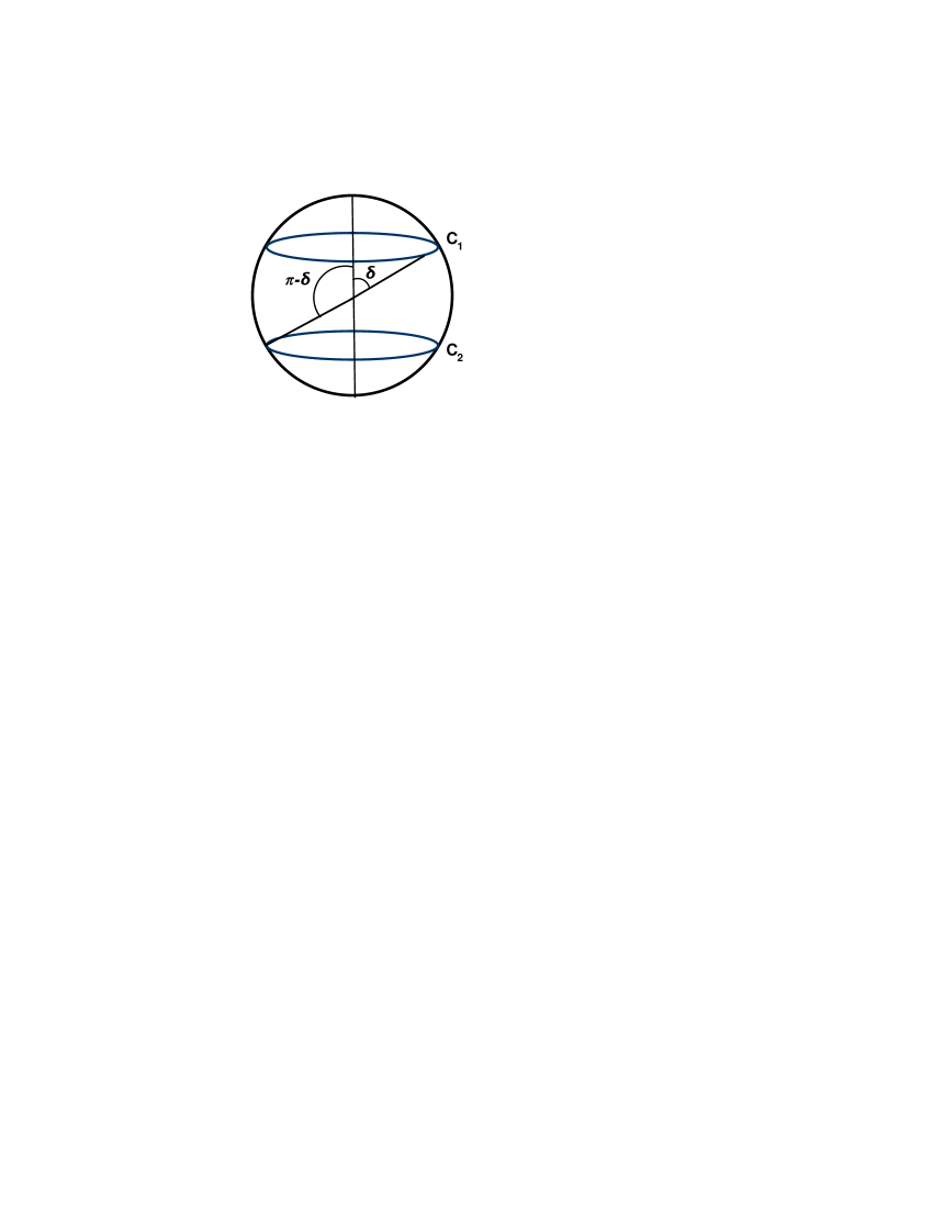
Figure 1: Symmetric configuration

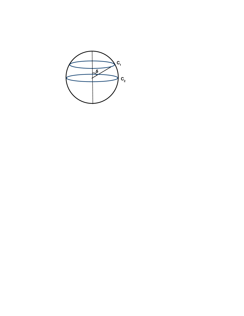
Figure 2: Asymmetric configuration

A general remark is in order. To have the errors under control we have limited our numerical analysis in the range $0.7\leq\delta\leq\pi/2$ for the symmetric case and for $1\leq\delta\leq\pi/2$ for the asymmetric case . Outside these two regions, i.e. for $0<\delta<0.7$ (symmetric case) and $0<\delta<1$ (asymmetric case) the requirement on the precision of the numerical integration becomes prohibitive for reasonable CPU times.

3.1 Ladder diagrams

To begin with, we shall consider all the diagrams which do not contain interactions. They can be naturally split into three families characterized by the number of field insertions at each latitude. Therefore, at order $g^{6}$ one has to consider the following possibilities: $g\cdot g^{5}$, $g^{2}\cdot g^{4}$ and $g^{3}\cdot g^{3}$.

$\mathbf{g\cdot g^{5}}$:

We have four diagrams with only one propagator insertion in one of the two latitudes and we have schematically listed them in fig. 3.

Figure 3: The four diagrams $g\cdot g^{5}$

Notice that the third and the fourth diagram can be obtained from the first two by exchanging the two latitudes ($C_{1}\leftrightarrow C_{2}$) and thus we have really to compute only two diagrams. In the following we shall denote with $t$ the angular parameter running over the latitude $C_{1}$ and with $s$, the one spanning the second latitude $C_{2}$. Then the contribution of the diagrams in fig. 3 can be summarized as follows

$$\mathbf{g^{1}\cdot g^{5}}= \frac{g^{6}}{N^{2}}\mathrm{P}\!\!\oint_{C_{1},C_{2}}\!\!\!dt_{1}\prod_{i=2}^{6}ds_{i}\langle\text{Tr}[\mathcal{A}(t_{1})]\text{Tr}[\mathcal{A}(s_{2})\mathcal{A}(s_{3})\mathcal{A}(s_{4})\mathcal{A}(s_{5})\mathcal{A}(s_{6})]\rangle_{0}+$$

$$+(C_{1}\leftrightarrow C_{2}),$$ (14)

where the symbol P in front of the integral means that the integration over the $s_{i}$ is ordered ($0\leq s_{6}\leq s_{5}\leq s_{4}\leq s_{3}\leq s_{2}\leq 2\pi$) and $\mathcal{A}$ stands for the usual effective connection constructed out of the gauge potential and the scalars. In (3.1) the vacuum expectation value is obviously taken in the free theory and by expanding it in terms of free propagators we find

$$\begin{split}\!\!\!\mathbf{g^{1}\cdot g^{5}}=&\frac{5\,g^{6}N}{4}\mathrm{P}\!\!\oint_{C_{1}C_{2}}\!\!\!dt_{1}\prod_{i=2}^{6}ds_{i}\Delta_{12}(t_{1},s_{2})\Delta_{22}(s_{3},s_{4})\Delta_{22}(s_{5},s_{6})+\\ &+\frac{5\,g^{6}}{8N}\mathrm{P}\!\!\oint_{C_{1}C_{2}}\!\!\!dt_{1}\prod_{i=2}^{6}ds_{i}\Delta_{12}(t_{1},s_{2})\Delta_{22}(s_{3},s_{5})\Delta_{22}(s_{4},s_{6})\,+(C_{1}\leftrightarrow C_{2}),\end{split}$$ (15)

where $\Delta_{12}(t_{i},s_{j})$ represents a propagator connecting the latitudes $C_{1}$ and $C_{2}$, while $\Delta_{11}(t_{i},t_{j})$ and $\Delta_{22}(s_{i},s_{j})$ denote an internal exchange on $C_{1}$ and $C_{2}$ respectively. Their explicit expression, if we use the polar representation for our circuits ($C_{1}=\{0,\sin\theta_{1}\sin t,\sin\theta_{1}\cos t,\cos\theta_{1}\}$, $C_{2}=\{0,\sin\theta_{2}\sin s,\sin\theta_{2}\cos s,\cos\theta_{2}\}$), is given by

$$\begin{split}&\Delta_{12}(t_{i},s_{j})=\frac{\sin\theta_{1}\sin\theta_{2}\left(\left(\cos\theta_{1}\cos\theta_{2}-1\right)\cos\left(t_{i}-s_{j}\right)+\sin\left(\theta_{1}\right)\sin\left(\theta_{2}\right)\right)}{8\pi^{2}\left(\sin\theta_{1}\sin\theta_{2}\cos\left(t_{i}-s_{j}\right)+\cos\theta_{1}\cos\theta_{2}-1\right)}\\ &\Delta_{11}(t_{i},t_{j})=-\frac{\sin^{2}\theta_{1}}{8\pi^{2}}\ \ \ \ \ \ \ \ \ \ \ \ \Delta_{22}(s_{i},s_{j})=-\frac{\sin^{2}\theta_{2}}{8\pi^{2}}.\end{split}$$ (16)

The integration over the two circuits can be easily performed in a closed form for two generic latitudes at $\theta=\theta_{1}$ and $\theta=\theta_{2}$ and we obtain the following compact expression

$$\mathbf{g^{1}\cdot g^{5}}=\frac{g^{6}(N+2N^{3})}{24A^{6}N^{2}}(A_{1}^{2}(A_{2}+A_{3})^{2}+A_{2}(A_{1}+A_{3})^{2})A_{1}A_{2},$$ (17)

in terms of the area $A_{1}$ ($A_{2}$) enclosed by the circuit $C_{1}$ ($C_{2}$) and the area $A_{3}$ delimited by the two latitudes. For our choice of configurations, the above expression yields the following two results

$$\mathbf{g^{1}\cdot g^{5}}=\left\{\begin{array}[]{ll}\textsc{symmetric:}&\frac{g^{6}(1+2N^{2})}{12N}\cos{\left(\frac{\delta}{2}\right)}^{4}\sin{\left(\frac{\delta}{2}\right)}^{8},\\ &\\ \textsc{asymmetric:}&\frac{g^{6}(1+2N^{2})}{6144N}\left(11-4\cos{\left(2\delta\right)}+\cos{\left(4\delta\right)}\right)\sin{\left(\frac{\delta}{2}\right)}^{2}.\end{array}\right.$$ (18)

$\mathbf{g^{2}\cdot g^{4}:}$

Again we have four diagrams with two propagator insertions in one of the two latitudes and they are shown in the fig. 4.

Figure 4: The four diagrams $g^{2}\cdot g^{4}$

Using the same conventions introduced for the previous case, the contribution of the above diagrams reads

$$\mathbf{g^{2}\cdot g^{4}}= \frac{g^{6}}{N^{2}}\,\mathrm{P}\!\!\oint_{C_{1}C_{2}}\!\!\!dt_{1}dt_{2}\prod_{i=3}^{6}ds_{i}\langle\text{Tr}[\mathcal{A}(t_{1})\mathcal{A}(t_{2})]\text{Tr}[\mathcal{A}(s_{3})\mathcal{A}(s_{4})\mathcal{A}(s_{5})\mathcal{A}(s_{6})]\rangle_{0}+$$

$$+(C_{1}\leftrightarrow C_{2}).$$ (19)

The symbol P denotes, this time, both the ordering in $t-$integration ($0\leq t_{2}\leq t_{1}\leq 2\pi$) and in the $s-$integration ($0\leq s_{6}\leq s_{5}\leq s_{4}\leq s_{3}\leq 2\pi$). If we expand the integrand of (3.1) in terms of free propagators, we obtain

$$\mathbf{g^{2}\cdot g^{4}}= \frac{g^{6}N}{2}\mathrm{P}\!\!\oint_{C_{1}C_{2}}\!\!\!dt_{1}dt_{2}\prod_{i=3}^{6}ds_{i}\Delta_{12}(t_{1},s_{3})\Delta_{12}(t_{2},s_{4})\Delta_{22}(s_{5},s_{6})\,+$$ (20)

$$+\frac{g^{6}}{4N}\mathrm{P}\!\!\oint_{C_{1}C_{2}}\!\!\!dt_{1}dt_{2}\prod_{i=3}^{6}ds_{i}\Delta_{12}(s_{1},s_{3})\Delta_{12}(t_{2},s_{5})\Delta_{22}(s_{4},s_{6})\,+(C_{1}\leftrightarrow C_{2}).$$

The above expression can be evaluated for generic latitudes and yields

$$\mathbf{g^{2}\cdot g^{4}}=\frac{g^{6}(N+2N^{3})}{12A^{6}N^{2}}(A_{1}A_{3}+A_{2}A_{3}+2A_{1}A_{2})A_{1}^{2}A_{2}^{2}\,\,.$$ (21)

For our particular choice of the configurations this formula reduces to

$$\mathbf{g^{2}\cdot g^{4}}=\left\{\begin{array}[]{ll}\textsc{symmetric:}&\frac{g^{6}(1+2N^{2})}{6N}\,\cos{\left(\frac{\delta}{2}\right)}^{2}\sin{\left(\frac{\delta}{2}\right)}^{10}\\ &\\ \textsc{asymmetric:}&-\frac{g^{6}(1+2N^{2})}{192N}\left(\cos{\left(\delta\right)}^{2}-2\right)\sin{\left(\frac{\delta}{2}\right)}^{4}.\end{array}\right.$$ (22)

$\mathbf{g^{3}\cdot g^{3}}$:

The remaining class of contributions in the absence of interaction is depicted in fig 5 and is given by

$$\mathbf{g^{3}\cdot g^{3}}= \frac{g^{6}}{N^{2}}\,\mathrm{P}\!\!\!\oint_{C_{1}C_{2}}\!\prod_{i=1}^{3}dt_{i}ds_{i+3}\langle\text{Tr}[\mathcal{A}(t_{1})\mathcal{A}(t_{2})\mathcal{A}(t_{3})]\text{Tr}[\mathcal{A}(s_{4})\mathcal{A}(s_{5})\mathcal{A}(s_{6})]\rangle_{0}\,+$$

$$+(C_{1}\leftrightarrow C_{2}).$$ (23)

Figure 5: The three diagrams $g^{3}\cdot g^{3}$.

For this family of graphs it is convenient to compute separately the three different contributions. The first one is similar to the diagrams considered in the previous cases. The sum of $\mathbf{D_{2}}$ and $\mathbf{D_{3}}$ in fig. 5 can be instead separated into the so-called abelian and maximally non-abelian part. To begin with, let us consider the diagram $\mathbf{D_{1}}$ which is given by

$$\mathbf{D_{1}}=\frac{g^{6}\,N}{32}\mathrm{P}\!\!\oint_{C_{1}C_{2}}\!\prod_{i=1}^{3}dt_{i}ds_{i+3}\Delta_{12}(t_{1},s_{4})\Delta_{11}(t_{2},t_{3})\Delta_{22}(s_{5},s_{6})\,+(C_{1}\leftrightarrow C_{2}).$$ (24)

Its evaluation is straightforward and one finds

$$\mathbf{D_{1}}=\frac{g^{6}N}{4A^{6}}(A_{2}+A_{3})(A_{1}+A_{3})A_{1}^{2}A_{2}^{2}=\left\{\begin{array}[]{ll}\textsc{symmetric:}&\frac{g^{6}N}{4}\cos{\left(\frac{\delta}{2}\right)}^{4}\sin{\left(\frac{\delta}{2}\right)}^{8}\\ &\\ \textsc{asymmetric:}&\frac{g^{6}N}{128}\sin{\left(\delta\right)}^{2}\sin{\left(\frac{\delta}{2}\right)}^{2}.\end{array}\right..$$ (25)

We come now to examine the abelian part, namely the part which is separately symmetric in $(t_{1},t_{2},t_{3})$ and $(s_{4},s_{5},s_{6})$. We can exploit this symmetry to eliminate the path-ordering in the integral and to write

$$\mathbf{Ab}=\frac{g^{6}}{48N}\,\oint_{C_{1}C_{2}}\!\prod_{i=1}^{3}dt_{i}ds_{i+3}\,\Delta_{12}(t_{1},s_{4})\Delta_{12}(t_{2},s_{5})\Delta_{12}(t_{3},s_{6}).$$ (26)

This integral is simply the cube of the single-exchange diagram and it value is

$$\mathbf{Ab}=\frac{g^{6}N}{6A^{6}N^{2}}A_{1}^{3}A_{2}^{3}=\left\{\begin{array}[]{ll}\textsc{symmetric:}&\frac{g^{6}}{6N}\sin{\left(\frac{\delta}{2}\right)}^{12}\\ &\\ \textsc{asymmetric:}&\frac{g^{6}}{48N}\sin{\left(\frac{\delta}{2}\right)}^{6}.\end{array}\right.$$ (27)

Finally, we have to compute the maximally non-abelian part, whose expression is given by

$$\mathbf{NAb}= \frac{g^{6}(N^{3}-N)}{4N^{2}}\mathrm{P}\oint_{C_{1}C_{2}}\!\prod_{i=1}^{3}dt_{i}ds_{i+3}\biggl{[}\Delta_{12}(t_{1},s_{4})\Delta_{12}(t_{2},s_{6})\Delta_{12}(t_{3},s_{5})\,+$$ (28)

$$+\Delta_{12}(t_{1},s_{5})\Delta_{12}(t_{2},s_{4})\Delta_{12}(t_{3},s_{6})\,+\Delta_{12}(t_{1},s_{6})\Delta_{12}(t_{2},s_{5})\Delta_{12}(t_{3},s_{4})\,\biggr{]}.$$

For two generic latitudes, we can perform five of the six integrations finding

$$\mathbf{NAb}= \frac{g^{6}(N^{3}-N)}{N^{2}}\left[\frac{J}{32\,\pi^{2}}\int_{0}^{2\pi}\!\!\!\!\!\!\,\frac{d\sigma\sigma^{2}(\cos{\theta_{1}}\cos{\theta_{2}}-1)(\cos{\theta_{2}}-\cos{\theta_{1}})^{3}}{\cos^{2}{\frac{\sigma}{2}}(\cos{\theta_{2}}-\cos{\theta_{1}})^{2}+(\cos{\theta_{1}}\cos{\theta_{2}}-1)^{2}\,\sin^{2}{\frac{\sigma}{2}}}-\right.$$

$$\left.-\frac{\pi J}{12}\left(\cos{\theta_{2}}\cos{\theta_{1}}-1)(-2\cos{\theta_{1}}+\cos{\theta_{2}}(\cos{\theta_{1}}+2)-1\right)+2\pi^{3}\,J^{\,3}\right]\equiv$$

$$\equiv \,\frac{g^{6}(N^{3}-N)}{N^{2}}\textsc{NAB}[\theta_{1},\theta_{2}],$$ (29)

where the constant $J$ is defined by

$$J=\int_{0}^{2\pi}ds\Delta_{12}(t,s).$$ (30)

Actually we could also perform the last integration in terms of $\mathrm{Li}_{2}(z)$, but for the subsequent numerical analysis this integral representation is more useful.

Let us collect the above results in a compact form. Apart from the maximally non-abelian contribution, all the other ladder graphs can be summed to give

$$\textsc{Lad}^{\textsc{sym/asym}}[\delta]=g^{6}N\textsc{Lad}^{\textsc{sym/asym}}_{N}[\delta]+\frac{g^{6}}{N}\textsc{Lad}^{\textsc{sym/asym}}_{1/N}[\delta],$$ (31)

where

$$\textsc{Lad}^{\textsc{sym}}_{N}[\delta]=\frac{5}{12}\cos{\left(\frac{\delta}{2}\right)}^{4}\sin{\left(\frac{\delta}{2}\right)}^{8}+\frac{1}{3}\cos{\left(\frac{\delta}{2}\right)}^{2}\sin{\left(\frac{\delta}{2}\right)}^{10},$$ (32a)

$$\textsc{Lad}^{\textsc{asym}}_{N}[\delta]=\small\frac{1}{3072}\sin^{2}\left(\frac{\delta}{2}\right)(47-20\cos(\delta)-24\cos(2\delta)+4\cos(3\delta)+\cos(4\delta)),$$ (32b)

$$\textsc{Lad}^{\textsc{sym}}_{1/N}[\delta]=\small\frac{1}{12}\cos{\left(\frac{\delta}{2}\right)}^{4}\sin{\left(\frac{\delta}{2}\right)}^{8}+\frac{1}{6}\cos{\left(\frac{\delta}{2}\right)}^{2}\sin{\left(\frac{\delta}{2}\right)}^{10}+\frac{1}{6}\sin{\left(\frac{\delta}{2}\right)}^{12},$$ (32c)

$$\textsc{Lad}^{\textsc{asym}}_{1/N}[\delta]=\small\frac{1}{6144}\sin^{2}\left(\frac{\delta}{2}\right)(83-84\cos(\delta)+4\cos(2\delta)+4\cos(3\delta)+\cos(4\delta)).$$ (32d)

The remaining maximally non-abelian part $\textsc{NAB}[\theta_{1},\theta_{2}]$ can be evaluated numerically with high precision starting from expression (29), with irrelevant numerical error.

3.2 Interaction diagrams

We now consider all the diagrams at order $g^{6}$ containing one or more interaction vertices. A partial analysis of this family of graphs was performed in [13] and [15] and in the following we heavily rely on the results of both papers. There it was shown how to reorganize the different contributions in order to get a result which is manifestly free of UV-divergences. In particular the diagrams were divided into three different classes [IY-diagram, H-diagram and X-diagram], which are separately finite.

 IY-diagram 

This term corresponds to the sum of graphs depicted in fig. 6: they contain both the vertex contributions and the one-loop bubble corrections. These diagram are separately UV divergent and in order to get a finite expression it is convenient to collect

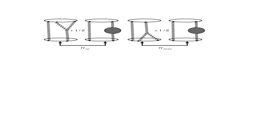
Figure 6: IY-diagram

them as illustrated in fig. 6. We shall call these two quantities $\mathrm{IY}_{\rm up}$ and $\mathrm{IY}_{\rm down}$. They are finite [15] and one can obtain one from the other by exchanging $C_{1}$ with $C_{2}$. For example the explicit expression for $\mathrm{IY}_{\rm up}$ was derived in [15] and it is given by

$$\mathbf{IY}_{\mathbf{up}}= \frac{\lambda^{3}J}{8N^{2}}\left[\int^{2\pi}_{0}d{t}_{1}d{t}_{2}d{t}_{3}d{s}_{2}\varepsilon({t}_{1},{t}_{2},{t}_{3})\right.\{(\dot{x}_{1}\circ\dot{y}_{2})2\dot{x}_{2}\cdot\partial_{y_{2}}-$$

$$\left.-(\dot{x}_{1}\circ\dot{x}_{2})\dot{y}_{2}\cdot\partial_{x_{2}}\}\mathcal{I}_{1}(x_{1},x_{2},y_{2})-2\int^{2\pi}_{0}d{t}_{1}d{t}_{2}d{s}_{2}(\dot{x}_{1}\circ\dot{y}_{2})\mathcal{I}_{1}(x_{1},x_{2},y_{2})\right].$$ (33)

Let us briefly recall the notation introduced in [13, 15]. Given two circuits $x(t)$ and $y(s)$ the effective scalar product $(\dot{x}\circ\dot{y})$ is a short-hand notation for $\dot{x}\cdot\dot{y}-|\dot{x}||\dot{y}|\Theta_{\dot{x}}\cdot\Theta_{\dot{y}}$, where $|\dot{x}|\Theta_{\dot{x}}^{I}=M_{I}^{i}\epsilon_{irs}\dot{x}^{r}x^{s}$. Here and in the following $x_{i}\equiv x(t_{i})$ and $y_{i}\equiv y(s_{i})$ will denote points on the upper and lower latitudes respectively. The function $\mathcal{I}_{1}(x_{1},x_{2},x_{3})$ carries the information about the integration over the position of the three vertex and it is defined by

$$\mathcal{I}_{1}(x_{1},x_{2},x_{3})=\int\frac{d^{4}z}{(2\pi)^{6}}\frac{1}{(x_{1}-z)^{2}(x_{2}-z)^{2}(x_{3}-z)^{2}}.$$ (34)

One can perform the integration over $z$ and one gets the following more useful expression in terms of one Feynman parameter:

$$\mathcal{I}_{1}(x_{1},x_{2},x_{3})=\frac{1}{64\pi^{2}}\int_{0}^{1}d\alpha\frac{{\log}\left(1+\frac{((x_{3}-x_{2})-\alpha(x_{1}-x_{2}))^{2}}{\alpha(1-\alpha)(x_{1}-x_{2})^{2}}\right)}{((x_{3}-x_{2})-\alpha(x_{1}-x_{2}))^{2}}.$$ (35)

Actually one can also perform the last integration in terms of ${\rm Li}_{2}(z)$, but the integral representation is more suitable for a numerical analysis. The expression for $\textrm{IY}_{down}$ is obtained by exchanging $x$ with $y$ and $t$ with $s$. The final step is to evaluate explicitly the integration over $t_{3}$ by means of the formula $\int_{0}^{2\pi}dt_{3}\epsilon(t_{1},t_{2},t_{3})=2\pi\mathrm{sign}(t_{1}-t_{2})-2(t_{1}-t_{2})$. If we define the function $\mathbf{IY}[\theta_{1},\theta_{2}]$ as follows

$${\rm IY}_{\rm up}+{\rm IY}_{\rm down}=\frac{g^{6}(N^{3}-N)}{N^{2}}\mathbf{IY}[\theta_{1},\theta_{2}],$$ (36)

its value can be computed numerically with the Montecarlo integration contained in Mathematica 7 both for the symmetric and for the asymmetric case.

 H-diagram 

The H-diagram is drawn in fig. 7. In [13, 15] its structure was analyzed in great detail. For two latitudes, the contribution of this diagram can be cast in the following simple form

Figure 7: H-diagram

$$\begin{split}\mathbf{H}=&-\frac{\lambda^{3}}{8N^{2}}\int d^{4}w\left[\underset{\mathbf{A}_{1}}{{P}^{M}(x_{1},y_{1},w){P}^{M}(x_{2},y_{2},w)}+\right.\\ &\ \ \ \ \ \ \ \ \ \ \ +\left.\underset{\mathbf{A_{2}}}{{Q}^{M}(x_{1},y_{1},w){Q}^{M}(x_{2},y_{2},w)}\right],\end{split}$$ (37)

where

$$P^{M} (x_{i},y_{i},w)=\int_{0}^{2\pi}\!\!\!\!\!\!d\tau_{i}d\sigma_{i}\left[2\dot{y_{i}}^{M}(\dot{x}_{i}\cdot\partial_{{y_{i}}}\mathcal{I}_{i}(x_{i},y_{i},w))-\right.$$

$$-\left.2\dot{x}_{i}^{M}(\dot{y_{i}}\cdot\partial_{x_{i}})\right]\frac{1}{(2\pi)^{4}(x_{i}-w)^{2}(y_{j}-w)^{2}}$$ (38)

and

$$Q^{M}(x_{i},y_{i},w)=\int_{0}^{2\pi}\!\!\!\!\!\!d\tau_{i}d\sigma_{i}(\dot{x}_{i}\circ\dot{y}_{i})(\partial_{x^{M}_{i}}-\partial_{y^{M}_{i}})\frac{1}{(2\pi)^{4}(x_{i}-w)^{2}(y_{j}-w)^{2}}.$$ (39)

In (37), (3.2) and (39), the index $M$ is a ten-dimensional label running from $1$ to $10$ and in particular we have defined $x^{M}\equiv(x^{\mu},i\Theta^{I}|\dot{x}|)$ and $\partial_{M}\equiv(\partial_{\mu},0)$. Let us compute first $\mathbf{A_{2}}$. It is convenient to rewrite this contribution as follows

$$\mathbf{A_{2}}=\frac{\lambda^{3}}{8N^{2}}\int_{0}^{2\pi}\!\!\!\!\!\!d\tau_{1}d\tau_{2}d\sigma_{1}d\sigma_{2}\dot{x}_{1}\circ\dot{y_{1}}\dot{x}_{2}\circ\dot{y_{2}}(\partial_{x_{1}}-\partial_{y_{1}})\cdot(\partial_{x_{2}}-\partial_{y_{2}})\mathcal{H}(x_{1},y_{1};x_{2},y_{2}),$$ (40)

where

$$\begin{split}\mathcal{H}(x_{1},y_{1};x_{2},y_{2})=&\frac{1}{(2\pi)^{10}}\int\frac{d^{4}zd^{4}w}{(x_{1}-z)^{2}(y_{1}-z)^{2}(z-w)^{2}(x_{2}-w)^{2}(y_{2}-w)^{2}}.\end{split}$$ (41)

The action of $(\partial_{x_{1}}-\partial_{y_{1}})\cdot(\partial_{x_{2}}-\partial_{y_{2}})$ on $\mathcal{H}(x_{1},y_{1};x_{2},y_{2})$ can then be evaluated with the identity (A.7) given in [27]. One finds

$$(\partial_{x_{1}}-\partial_{y_{1}})\cdot(\partial_{x_{2}}-\partial_{y_{2}})\mathcal{H}(x_{1},y_{1};x_{2},y_{2})=$$

$$= \frac{1}{(x_{1}-y_{1})^{2}(x_{2}-y_{2})^{2}}\biggl{[}\mathcal{I}^{(4)}(x_{1},y_{1},x_{2},y_{2})((x_{1}-x_{2})^{2}(y_{1}-y_{2})^{2}-(x_{1}-y_{2})^{2}(x_{2}-y_{1})^{2})$$

$$+\frac{1}{(2\pi)^{2}}(Y(x_{1},x_{2},y_{2})-Y(y_{1},x_{2},y_{2})+Y(x_{2},x_{1},y_{1})-Y(y_{2},x_{1},y_{1}))\biggr{]},$$ (42)

where ${Y}(x_{1},x_{2},x_{3})\equiv{\mathcal{I}_{1}(x_{1},x_{2},x_{3})}[(x_{1}-x_{3})^{2}-(x_{1}-x_{2})^{2}].$ Both in the symmetric and asymmetric case the integration over the circuits can now be carried numerically and one determines the color-stripped contribution $\mathbf{A2}[\theta_{1},\theta_{2}]$ defined by

$$\mathbf{A_{2}}=\frac{g^{6}(N^{3}-N)}{N^{2}}\mathbf{A2}[\theta_{1},\theta_{2}].$$ (43)

Next we consider the evaluation of the $\mathbf{A_{1}}$ contribution. This time we shall follow a different path in our analysis, namely we shall first perform the integration over the circuit analytically and then we perform numerically the integration over the position of the vertices. The first step is to study the function $P^{M}(w)$. The only non-vanishing components are $M=4,5$

$$P^{4}(w)= -2i\sin{{\theta_{1}}}\sin{{\theta_{2}}}(\cos{{\theta_{1}}}-\cos{{\theta_{2}}})\left(I_{s}({\theta_{2}})\partial_{w_{0}}I_{c}({\theta_{1}})-I_{c}({\theta_{2}})\partial_{w_{0}}I_{s}({\theta_{1}})\right),$$ (44a)

$$P^{5}(w)= -2i\sin{{\theta_{1}}}\sin{{\theta_{2}}}(\cos{{\theta_{1}}}-\cos{{\theta_{2}}})\left(I_{s}({\theta_{2}})\partial_{w_{1}}I_{c}({\theta_{1}})-I_{c}({\theta_{2}})\partial_{w_{1}}I_{s}({\theta_{1}})\right).$$ (44b)

The function $I_{c}(\delta)$ and $I_{s}(\delta)$ are given in appendix C. In summary, we have to evaluate

$$\mathbf{A_{1}}=\frac{g^{6}N(N^{2}-1)}{8N^{2}}\int d^{4}wd^{4}z\frac{P^{4}(w)P^{4}(z)+P^{5}(w)P^{5}(z)}{(w-z)^{2}}.$$ (45)

Two of the eight integrations can be performed analytically (we do not present the cumbersome result): if we set

$$\mathbf{A_{1}}=\frac{g^{6}N(N^{2}-1)}{8N^{2}}\mathbf{A1}[\theta_{1},\theta_{2}],$$ (46)

the remaining six integrals defining the quantity $\mathbf{A1}[\theta_{1},\theta_{2}]$ can be computed numerically. This step is the most delicate one and the most unstable from the point of view of the convergence of the numerical integration. As discussed in the introduction, the reason why we limited our analysis to the region $0.7\leq\delta\leq\pi/2$ for the symmetric case and to the region $1\leq\delta\leq\pi/2$ for the asymmetric case is the requirement to have reliable results using the Montecarlo integration routine present in Mathematica 7.

Figure 8: X-diagram

 X-diagram 

There is final diagram to be considered: the so-called X-diagram (see fig. 8). Its expression is quite compact and it is given by

$$\begin{split}&\mathbf{X}=\frac{g^{6}N(N^{2}-1)}{8(4\pi^{2})^{4}}\int_{0}^{2\pi}dt_{1}dt_{2}ds_{1}ds_{2}\times\\ &\times\int d^{4}w\frac{\left(\dot{x_{1}}\circ\dot{y_{2}})(\dot{x_{2}}\circ\dot{y_{1}})-(\dot{x_{1}}\circ\dot{x_{2}})(\dot{y_{2}}\circ\dot{y_{1}}\right)}{(x_{1}-w)^{2}(x_{2}-w)^{2}(y_{1}-w)^{2}(y_{2}-w)^{2}}.\end{split}$$ (47)

For the numerical evaluation the most convenient thing to do is to perform, first, the integration over the contours. Evaluating the integrals over the two circuits, for two generic latitudes we obtain the following expression in terms of $I[\delta]$, $I_{c}[\delta]$ and $I_{s}[\delta]$ described in appendix C

$$\mathbf{X}=\frac{g^{6}N(N^{2}-1)}{8(4\pi^{2})^{4}N^{2}}\!\!\!\int\!\!\!d^{4}w\sin^{4}{{\theta_{1}}}\sin^{4}{{\theta_{2}}}[(I({\theta_{1}})^{2}-I_{c}({\theta_{1}})^{2}-I_{s}({\theta_{1}})^{2})(I_{c}({\theta_{2}})^{2}+$$

$$+I_{s}({\theta_{2}})^{2}-I({\theta_{2}})^{2})]+[\sin{{\theta_{1}}}\sin{{\theta_{2}}}(1-\cos{{\theta_{1}}}\cos{{\theta_{2}}})(I_{c}({\theta_{1}})I_{c}({\theta_{2}})+$$

$$+I_{s}({\theta_{1}})I_{s}({\theta_{2}}))-\sin^{2}{{\theta_{1}}}\sin^{2}{{\theta_{2}}}I({\theta_{1}})I({\theta_{2}})]^{2}.$$ (48)

If we define the function $\mathbf{X}[\theta_{1},\theta_{2}]$ as

$$\mathbf{X}=\frac{g^{6}N(N^{2}-1)}{N^{2}}\mathbf{X}[\theta_{1},\theta_{2}],$$ (49)

for our specific configurations we can proceed with the numerical integration without encountering particular problems.

3.3 Comparison with $\mathbf{YM_{2}}$

We can now compare our numerical result with the analytic prediction given by two-dimensional Yang-Mills theory. Let us sum first all the contributions computed in the numerical analysis. The result is summarized for the symmetric case in fig. 10 and 10 while the asymmetric case is given in fig. 12 and 12.

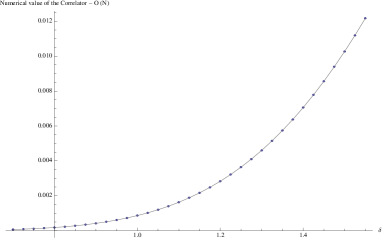
Figure 9: symmetric case: Leading contribution $g^{6}N$. The points are the results of the numerical analysis, while the light gray line is the QCD₂ prediction.

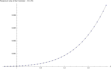
Figure 10: symmetric case Sub-leading contribution $g^{6}/N$. The points are the results of the numerical analysis, while the light gray line is the QCD₂ prediction.

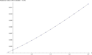
Figure 11: asymmetric case: Leading contribution $g^{6}N$. The points are the results of the numerical analysis, while the light gray line is the QCD₂ prediction.

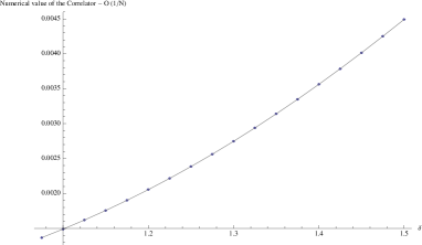
Figure 12: asymmetric case Sub-leading contribution $g^{6}/N$. The points are the results of the numerical analysis, while the light gray line is the QCD₂ prediction.

The prediction in the present two cases can be derived easily from the general expression for the correlator in the zero instanton sector given in [15] and reported here in (12). For the symmetric case we find

$$\langle WW\rangle_{g^{6}}=\frac{g^{6}N}{24}(5+4\cos{\delta}+\cos{\delta}^{2})\sin{\left(\frac{\delta}{2}\right)^{8}}+\frac{g^{6}}{12N}\sin{\left(\frac{\delta}{2}\right)^{8}},$$ (50)

while for the asymmetric case we obtain

$$\begin{split}\langle WW\rangle_{g^{6}}=&\frac{g^{6}N}{3072}\left(\sin\left(\frac{\delta}{2}\right)^{2}(-36\cos(\delta)-20\cos(2\delta)+4\cos(3\delta)+\cos(4\delta)+59)\right)+\\ &\frac{g^{6}}{6144N}\left(\sin^{2}\left(\frac{\delta}{2}\right)(-52\cos(\delta)-4\cos(2\delta)+4\cos(3\delta)+\cos(4\delta)+59)\right).\end{split}$$ (51)

In order to compare the results presented in figs 10, 10, 12 and 12 with the answer of matrix model, we compute the difference $\Delta_{\rm Cal-Pred}$ between the calculated values and the predicted ones. The results of this analysis are plotted in figs. 14, 14, 16 and 16, where the bar denotes the estimated errors. We see that the difference from the central value $0$ is quite small. It is easy to see that the average absolute error is of order $10^{-6}$ / $10^{-7}$, the relative error is of the order $10^{-4}$ at worst.

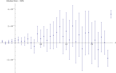
Figure 13: symmetric case: $\Delta_{\rm Cal-Pred}$ at the leading contribution $g^{6}N$

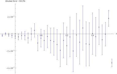
Figure 14: symmetric case $\Delta_{\rm Cal-Pred}$ at the sub-leading contribution $g^{6}/N$

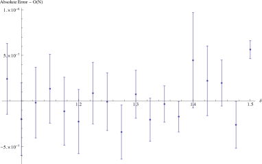
Figure 15: asymmetric case: $\Delta_{\rm Cal-Pred}$ at the leading contribution $g^{6}N$

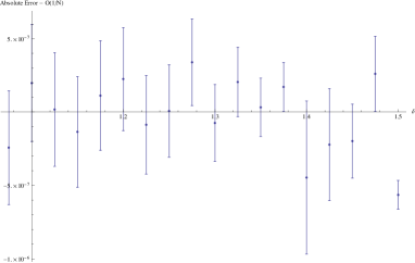
Figure 16: asymmetric case $\Delta_{\rm Cal-Pred}$ at the sub-leading contribution $g^{6}/N$

We also note that the error bars increase as the coincident limit is approached. This is a generic feature of the calculation as the integrands become increasingly singular in this limit. Conversely, the error is relatively small for small $\delta$, however the precision required to reliably calculate certain integrals in this “shrinking” limit becomes prohibitive for $\delta$ less than about 0.7 (1.0), in the symmetric case (asymmetric case), and this defines the lower bound of our chosen range. We thus conclude that the conjecture is verified with a relative error of order $10^{-4}$ in the range $0.7\leq\delta\leq\pi/2$ for the symmetric case and in the range $1\leq\delta\leq\pi/2$ for the asymmetric case.

4 Correlator at strong coupling from supergravity

At strong coupling, the AdS/CFT correspondence may be used to compute the correlator between two Wilson loops in ${\cal N}=4$ SYM [28]. Practically, by taking the limit in which the separation of the two Wilson loops is much larger than their sizes, and working at large $N$, the correlator is computed by calculating the exchange of light supergravity fluctuations between the Wilson loop worldsheets. At infinite separation, only the lightest fluctuation modes need be considered; the subleading contributions stemming from the relaxation of this limit are given by the exchange of heavier modes. In [15], the contributions to the correlator from a class of modes (dual to the ${\cal N}=4$ SYM chiral primary operators $\text{Tr}(\Phi_{3}+i\Phi_{4})^{J}$) which includes a representative of the lightest modes (i.e. for $J=2$) were presented. It was found that the contribution of this $J=2$ mode alone matched the infinite separation limit of the YM₂ result. Beyond this, a remarkable pattern of matching between contributions from the modes dual to $\text{Tr}(\Phi_{3}+i\Phi_{4})^{J}$ for general $J$, and corresponding terms in the YM₂ expression for the correlator was uncovered. This remarkable pattern of matching terms has since been corroborated using the techniques of localization [22], where it was shown that the localization conditions equate the superprotected operator appearing in the Wilson loop’s OPE expansion discovered in [15] to precisely the chiral primary operator referred to above.

Beyond this pattern of matching terms, at respectively subleading orders in the large separation limit, the contributions of the aforementioned dual chiral primary modes also include terms absent from the YM₂ result. One would expect these terms to be removed, i.e. cancelled, by the inclusion of the other supergravity modes which are respectively heavier, order-by-order, compared to the dual chiral primaries.

In fact a problem emerges before this. In a correlator calculation we are instructed to sum over the exchange of all possible modes. Let us concentrate on the bottom of the spectrum. In addition to the mode dual to $\text{Tr}(\Phi_{3}+i\Phi_{4})^{2}$, one must also include the mode dual to the conjugate operator $\text{Tr}(\Phi_{3}-i\Phi_{4})^{2}$, and to the orthogonal operators $\text{Tr}(\Phi_{3}^{2}+\Phi_{4}^{2}-\Phi_{5}^{2}-\Phi_{6}^{2})$ and $\text{Tr}(3(\Phi_{1}^{2}+\Phi_{2}^{2})-1)$. These correspond in the supergravity picture to various $S^{5}$ spherical harmonics of weight 2. These extra modes contribute at the leading order in the large-separation limit, and in order not to spoil the agreement with YM₂ should be cancelled by yet other modes.

It happens that there are two types of further supergravity fluctuations around $AdS_{5}\times S^{5}$ which could potentially do the job. These are the leading fluctuations of the NS-NS B-field with legs in the $AdS_{5}$ and $S^{5}$ directions respectively [29][31]. They are dual to the following gauge theory operators (see appendix A of [32])

$$\begin{split}&\psi_{A}\psi_{B}~{}~{}\rightarrow~{}~{}\text{B-field on $S^{5}$},\\ &\bar{\psi}^{A}\sigma_{\mu\nu}\bar{\psi}^{B}+2i\Phi^{AB}F^{+}_{\mu\nu}~{}~{}\rightarrow~{}~{}\text{B-field on $AdS_{5}$}.\end{split}$$ (52)

The coupling of these operators has been discussed previously in the context of the 1/2 BPS circular Wilson loop [33][34]. We will find that they provide leading contributions of the right order and sign, but fail to cancel the offending chiral primary contributions due to mismatched coefficients. By going higher in the supergravity spectrum, we have verified that the next heaviest modes all contribute beyond the leading order and are thus powerless to save the agreement with YM₂.

The interpretation of the disagreement is not clear. It could be that there is a problem with the supergravity limit in this instance, and that string modes are surviving and contributing to the correlator. The strong coupling limit here could be subtle, since we are considering Wilson loops in the limit in which they become the supersymmetric circles of Zarembo [35], where the rescaled coupling in the matrix model approaches zero [36]. Of course, there is also the possibility that the YM₂-DGRT [11] Wilson loop equivalence needs to be adjusted at strong coupling, perhaps through the effects of the undetermined 1-loop determinant appearing in the localization formulae [18]. There may also be a subtlety with the supergravity calculations themselves. In the remainder of this section we present these supergravity calculations in detail, and leave the resolution of the puzzle of disagreement to future work.

4.1 Preliminaries

The fundamental string solution corresponding to the latitude DGRT Wilson loop was provided in [11]. We write the metric of $AdS_{5}\times S^{5}$ as

$$ds^{2}=\Biggl{(}\frac{dy^{2}+dr^{2}+r^{2}d\phi^{2}+dx^{2}+dz^{2}}{y^{2}}+\cos^{2}\vartheta\,d\Omega_{3}^{2}+d\vartheta^{2}+\sin^{2}\vartheta\,d\varphi^{2}\Biggr{)}$$ (53)

where the angle $\vartheta\in[0,\pi/2]$. The worldsheet coordinates are $\sigma\in[0,\infty)$ and $\tau\in[0,2\pi)$. The embedding functions are $z=d\Omega_{3}=0$ and

$$y=\sin\theta_{i}\,\tanh\sigma,\quad r=\frac{\sin\theta_{i}}{\cosh\sigma},\quad\phi=\tau,\quad x=\cos\theta_{i},\quad\sin\vartheta=\frac{1}{\cosh(\sigma+\sigma_{i})},\quad\varphi=\tau-\pi,$$ (54)

where $\theta_{i}$ is the position of the latitude on the sphere, i.e. its radius. Note that the latitude’s path on the internal-space sphere is also a latitude, albeit at

$$\vartheta_{i}=\frac{\pi}{2}-\theta_{i}$$ (55)

and so

$$\sin\vartheta_{i}=\frac{1}{\cosh\sigma_{i}}=\cos\theta_{i}.$$ (56)

We would like to compute the correlator between two such latitudes at polar angles $\theta_{0}$ and $\theta_{1}$, in the limit $\theta_{0}\to 0$, $\theta_{1}\to\pi$. In the rest of the document we take $\theta_{1}\to\pi-\theta_{1}$, so that small $\theta_{1}$ indicates a latitude close to the south pole of the $S^{2}$.

4.2 Dual chiral primaries

The supergravity modes that we are interested in are fluctuations of the RR 5-form as well as the spacetime metric. They are by now very well known, and details can be found in [28][37][29][30][39]. The fluctuations are

$$\delta g_{\mu\nu} = \left[-\frac{6\,J}{5}\,g_{\mu\nu}+\frac{4}{J+1}\,D_{(\mu}D_{\nu)}\right]\,s^{J}(X)\,Y_{J}(\Omega),$$ (57)

$$\delta g_{\alpha\beta} = 2\,J\,g_{\alpha\beta}\,s^{J}(X)\,Y_{J}(\Omega),$$ (58)

where $\mu,\nu$ are $AdS_{5}$ and $\alpha,\beta$ are $S^{5}$ indices. The symbol $X$ indicates coordinates on $AdS^{5}$ and $\Omega$ coordinates on the $S^{5}$. The $D_{(\mu}D_{\nu)}$ represents the traceless symmetric double covariant derivative. The $Y_{J}(\Omega)$ are the spherical harmonics on the five-sphere, while $s^{J}(X)$ have arbitrary profile and represent a scalar field propagating on $AdS_{5}$ space with mass squared $=J(J-4)$, where $J$ labels the representation of $SO(6)$ and must be an integer greater than or equal to 2.

The bulk-to-bulk propagator for $s^{J}$ is given in [28], with normalization from [37]. It is expressed in terms of a hypergeometric function

$$\begin{split}&P(X,\bar{X})=\frac{\alpha_{0}}{B_{J}}\,W^{J}\,{{}_{2}}F_{1}(\,J,\,J-3/2,\,2J-3;\,-4W),\\ &W=\frac{y\bar{y}}{(y-\bar{y})^{2}+(x-\bar{x})^{2}+(z-\bar{z})^{2}+r^{2}+\bar{r}^{2}-2r\bar{r}\cos(\phi-\bar{\phi})},\end{split}$$ (59)

where,

$$\begin{split}\alpha_{0}=\frac{J-1}{2\pi^{2}},\qquad&B_{J}=\frac{2^{3-J}N^{2}J(J-1)}{\pi^{2}(J+1)^{2}}.\end{split}$$ (60)

Given (57) and (53), we must construct the traceless symmetric double covariant derivative,

$$D_{(\mu}D_{\nu)}\equiv\frac{1}{2}\left(D_{\mu}D_{\nu}+D_{\nu}D_{\mu}\right)-\frac{1}{5}g_{\mu\nu}\,g^{\rho\sigma}D_{\rho\sigma},$$ (61)

the details of which are given in appendix B. Then, using a 10-d index $M=(\mu,\alpha)$, we can express the metric fluctuations as $\delta g_{MN}=\delta\tilde{g}_{MN}\,s^{J}Y_{J}$, where

$$\begin{split}&\delta\tilde{g}_{yy}=\frac{4}{J+1}\left[\partial_{y}^{2}+\frac{1}{y}\partial_{y}\right]-\frac{2J}{y^{2}}\frac{(J-1)}{(J+1)},~{}~{}\delta\tilde{g}_{rr}=\frac{4}{J+1}\left[\partial_{r}^{2}-\frac{1}{y}\partial_{y}\right]-\frac{2J}{y^{2}}\frac{(J-1)}{(J+1)},\\ &\delta\tilde{g}_{yr}=\frac{4}{J+1}\left[\partial_{y}\partial_{r}+\frac{1}{y}\partial_{r}\right],~{}~{}\delta\tilde{g}_{\phi\phi}=\frac{4}{J+1}\left[\partial_{\phi}^{2}-\frac{r^{2}}{y}\partial_{y}+r\partial_{r}\right]-r^{2}\frac{2J}{y^{2}}\frac{(J-1)}{(J+1)},\\ &\delta\tilde{g}_{\vartheta\vartheta}=2J,~{}~{}\delta\tilde{g}_{\varphi\varphi}=2J\sin^{2}\vartheta,\end{split}$$ (62)

and where we have used the fact that $D^{2}s^{J}=J(J-4)s^{J}$. We may now assemble the expression for the correlator

$$\frac{\langle W(x)\,W(\bar{x})\rangle}{\langle W(x)\rangle\langle W(\bar{x})\rangle}=\left(\frac{\sqrt{\lambda}}{4\pi}\right)^{2}\int_{\Sigma}\int_{\bar{\Sigma}}\partial_{a}X^{M}\partial^{a}X^{N}\,\delta g_{MN}\,P(X,\bar{X})\,\delta\bar{g}_{\bar{M}\bar{N}}\,\partial_{\bar{a}}X^{\bar{M}}\partial^{\bar{a}}X^{\bar{N}}.$$

As explained at the start of this section (see also appendix A), at the level of $J=2$, we have four states which couple to the Wilson loops. They correspond to the following scalar spherical harmonics on $S^{5}$

$$\begin{split}&Y^{2,2}_{0,+2,0}=\frac{1}{2}\cos^{2}\vartheta\sin^{2}\vartheta_{2}\,e^{2i\varphi_{2}},~{}~{}Y^{2,2}_{0,-2,0}=\frac{1}{2}\cos^{2}\vartheta\sin^{2}\vartheta_{2}\,e^{-2i\varphi_{2}},\\ &Y^{2,0}_{0,0,0}=\frac{1}{2\sqrt{3}}\left(3\sin^{2}\vartheta-1\right),~{}~{}~{}Y^{2,2}_{0,0,0}=-\frac{1}{2}\cos^{2}\vartheta\cos 2\vartheta_{2}.\end{split}$$ (63)

On the string solution we have $\vartheta_{2}=\pi/2,\varphi_{2}=0$, and so these harmonics reduce to

$$Y^{2,2}_{0,+2,0}=Y^{2,2}_{0,-2,0}=Y^{2,2}_{0,0,0}=\frac{1}{2}\cos^{2}\vartheta,\qquad Y^{2,0}_{0,0,0}~{}\text{unchanged}.$$ (64)

We find the following results (higher order results for $Y^{J,J}_{0,\pm J,0}$ for $J=2,3,4$ have been presented in [15]; here we are interested in the leading order in $\theta_{0},\theta_{1}$ which is given by $J=2$)

$$\begin{split}&\frac{\langle W(x)\,W(\bar{x})\rangle}{\langle W(x)\rangle\langle W(\bar{x})\rangle}\Biggr{|}_{\frac{1}{2}\cos^{2}\vartheta}=\frac{\lambda}{8N^{2}}\Biggl{[}\frac{\theta_{0}^{3}\,\theta_{1}^{3}}{2^{2}}+{\cal O}(\theta^{10})\Biggr{]},\\ &\frac{\langle W(x)\,W(\bar{x})\rangle}{\langle W(x)\rangle\langle W(\bar{x})\rangle}\Biggr{|}_{Y^{2,0}_{0,0,0}}=\frac{\lambda}{10N^{2}}\Biggl{[}\frac{13\,\theta_{0}^{4}\,\theta_{1}^{4}}{5\cdot 3^{2}}+\frac{3(\theta_{0}^{4}\,\theta_{1}^{5}+\theta_{0}^{5}\,\theta_{1}^{4})}{2^{4}}+{\cal O}(\theta^{10})\Biggr{]},\end{split}$$ (65)

where ${\cal O}(\theta^{n})$ is shorthand for terms of the form $\theta_{0}^{p}\theta_{1}^{q}$ where $p+q\geq 10$. The result coming from YM₂ in the large $\lambda,N$ limit is given by [15][14]

$$\frac{\langle W(x)\,W(\bar{x})\rangle}{\langle W(x)\rangle\langle W(\bar{x})\rangle}\Biggr{|}_{YM_{2}}=\frac{\lambda}{8N^{2}}\Biggl{[}\frac{\theta_{0}^{3}\,\theta_{1}^{3}}{2^{2}}+{\cal O}(\theta^{10})\Biggr{]},$$ (66)

and so matches the contribution of one of the three modes $Y^{2,2}_{0,+2,0},\,Y^{2,2}_{0,-2,0},\,Y^{2,2}_{0,0,0}$. The other two modes give contributions which left uncanceled spoil the agreement with YM₂. The $Y^{2,0}_{0,0,0}$ mode contributes at subleading order, i.e. $\theta_{0}^{4}\theta_{1}^{4}$, and so doesn’t concern us here. In the next sections we will consider the fluctuations of the B-field which we will find also lead as $\theta_{0}^{3}\theta_{1}^{3}$. However we will find that they do not remove the extra two contributions of the first line in (LABEL:CR).

4.3 NS-NS B-field on $S^{5}$

Continuing up the spectrum, the next lightest modes (outside of the $s^{J}$) stem from the fluctuation of the NS-NS B-field which can have both legs in either the $S^{5}$, or the $AdS_{5}$ directions, see eq. (2.48) and what follows it in [29]. Here we treat the $S^{5}$ directions, whose fluctuations correspond to an $AdS_{5}$ scalar field

$$\delta B_{\alpha\beta}=a^{k}_{-}(x)\,Y_{[\alpha\beta]}^{k,-}(\Omega),\qquad m_{a^{k}_{-}}^{2}=k^{2}-4.$$ (67)

The conformal dimension $\Delta$ of an operator related to a scalar field on $AdS_{d+1}$ with mass $m$ is given by

$$\Delta=\frac{d}{2}+\sqrt{m^{2}+\frac{d^{2}}{4}}.$$ (68)

Thus here we have

$$\Delta=k+2.$$ (69)

The $k=1$ mode thus corresponds to a gauge theory operator of dimension 3, in the ${\bf 10}$ of SU(4). Consulting appendix A of [32], we find that the operator is ${\cal E}_{AB}=\psi_{A}\psi_{B}$.

The antisymmetric tensor spherical harmonics $Y_{[\alpha\beta]}^{k,\pm}(\Omega)$ obey the following equations

$${\epsilon_{\alpha\beta}}^{\gamma\delta\lambda}\partial_{\gamma}Y_{[\delta\lambda]}^{k,\pm}=\pm 2i(k+2)\,Y_{[\alpha\beta]}^{k,\pm},\qquad\left(-\nabla^{2}_{S^{5}}+6\right)\,Y_{[\alpha\beta]}^{k,\pm}=(k+2)^{2}\,Y_{[\alpha\beta]}^{k,\pm},$$ (70)

and may are constructed using the (regular) tensor spherical harmonics given by

$$Y^{k}_{[\alpha\beta]}=\partial_{\alpha}x^{i}\,\partial_{\beta}x^{j}\,C_{[ijl_{1}](l_{2}\cdots l_{k})}\,x^{l_{1}}\cdots x^{l_{k}},$$ (71)

where $C$ is antisymmetric in $i,j,l_{1}$, symmetric in $l_{2},\ldots,l_{k}$, and traceless on any pair of indices. Using the complex basis (106), the $Y_{[\alpha\beta]}^{k,\pm}$ amount to a choice of sign for the charges associated with the angles $\varphi,\varphi_{2},\varphi_{3}$. As it turns out, our Wilson loop couples only to $\delta B_{\vartheta\varphi}$ and so we require only $Y^{1,-}_{[\vartheta,\varphi]}$. There are only two modes, given by

$$\begin{split}Y^{1,-}_{[\vartheta,\varphi]}=\sin\vartheta\sin\vartheta_{2}\,e^{-i\varphi_{2}},\qquad Y^{1^{\prime},-}_{[\vartheta,\varphi]}=\sin\vartheta\cos\vartheta_{2}\,e^{-i\varphi_{3}},\end{split}$$ (72)

where we have not yet normalized the spherical harmonics. Only the first will be non-zero on the string worldsheet.

The quadratic action for these fluctuations has been given in [40], see eq. (4.3) therein. One has

$$\begin{split}S=\frac{2}{2\kappa^{2}}\int d^{10}x\sqrt{g}\Biggl{(}\frac{1}{2}\Bigl{[}\partial_{\mu}B^{*}_{\alpha\beta}\,\partial^{\mu}B^{\alpha\beta}+\nabla_{\gamma}B^{*}_{\alpha\beta}\nabla^{\gamma}B^{\alpha\beta}&+6\,B^{*}_{\alpha\beta}B^{\alpha\beta}\Bigr{]}\\ &-i\epsilon^{\alpha\beta\gamma\delta\epsilon}B^{*}_{\alpha\beta}\,\partial_{\gamma}B_{\delta\epsilon}\Biggr{)},\end{split}$$ (73)

where, in units where the radius of $AdS_{5}$ is unity, $1/(2\kappa^{2})=4N^{2}/(2\pi)^{5}$. Subbing-in (67), we find

$$S=2C_{k}\,\frac{4N^{2}}{(2\pi)^{5}}\,\int_{AdS_{5}}d^{5}x\sqrt{g}\Biggl{(}\frac{1}{2}\Bigl{[}\partial_{\mu}a^{k,-}\,\partial^{\mu}a^{k,-}+m^{2}_{a^{k,-}}\left(a^{k,-}\right)^{2}\Bigr{]}\Biggr{)},$$ (74)

where the constant $C_{k}$ encodes the normalization of the spherical harmonics. Specifically one has

$$\begin{split}&C_{1}=\int d\Omega_{5}\,g^{\vartheta\vartheta}g^{\varphi\varphi}\,\left|Y^{1,-}_{[\vartheta,\varphi]}\right|^{2}=\frac{\pi^{3}}{2}.\\ \end{split}$$ (75)

Thus the propagator is given by

$$P=\frac{\tilde{\alpha}_{0}}{\tilde{B}_{k}}\,W^{\Delta}\,{{}_{2}}F_{1}(\Delta,\Delta-3/2,2\Delta-3;-4W)$$ (76)

where $\tilde{\alpha}_{0}=(\Delta-1)/(2\pi^{2})$, and $\tilde{B}_{k}=8N^{2}\,C_{k}/(2\pi)^{5}$. See section 4.2 for the definition of $W$.

Coupling to the string worldsheet, we have

$$\begin{split}\delta S&=i\frac{\sqrt{\lambda}}{4\pi}\int d^{2}\sigma\,\epsilon^{ab}\partial_{a}X^{M}\partial_{b}X^{N}\delta B_{MN}=-i\frac{\sqrt{\lambda}}{2\pi}\int d\sigma d\tau\,\vartheta^{\prime}\,\delta B_{\vartheta\varphi}\\ &=i\frac{\sqrt{\lambda}}{2\pi}\int d\sigma d\tau\,\sin\vartheta\,\delta B_{\vartheta\varphi},\end{split}$$ (77)

where a factor of $i$ has been included due to the Euclidean signature of the worldsheet. Evaluating the contribution of the $k=1$ mode to the correlator we find

$$\begin{split}\left.\frac{\langle W(x)\,W(\bar{x})\rangle}{\langle W(x)\rangle\langle W(\bar{x})\rangle}\right|_{\delta B_{\alpha\beta}}=-\frac{\lambda}{N^{2}}\frac{1}{2^{4}}\left(\frac{\theta_{0}^{3}\theta_{1}^{3}}{8}-\frac{(\theta_{0}^{3}\theta_{1}^{4}+\theta_{0}^{4}\theta_{1}^{3})}{5}\right)+{\cal O}(\theta^{8}).\\ \end{split}$$ (78)

It is straightforward to further evaluate the $k=2$ contributions. They lead as $\theta_{0}^{4}\theta_{1}^{4}$ and so don’t concern us here.

4.4 NS-NS B-field on $AdS_{5}$

The supergravity action for fluctuations of the NS-NS B field with both legs in the $AdS_{5}$ directions has been worked out in [40], while the dual gauge theory operator (for the lightest mode) has been discussed in [31]. The AdS/CFT correspondence relates linear combinations of the Ramond-Ramond 2-form potential $C_{\mu\nu}$ and the NS-NS B field $B_{\mu\nu}$ to dual operators in the gauge theory [40]

$$A=\sqrt{2}(B+iC),\quad\bar{A}=\sqrt{2}(B-iC),\quad B=\frac{1}{2\sqrt{2}}(A+\bar{A}),\quad C=\frac{1}{2\sqrt{2}i}(A-\bar{A}),$$ (79)

for which the action of the modes with both legs in the $AdS_{5}$ directions is given by

$$\begin{split}S&=\int d^{10}x\sqrt{-g}\Bigl{(}-\frac{1}{2}\left(\nabla_{\mu}\bar{A}_{\nu\rho}(\nabla^{\mu}A^{\nu\rho}-\nabla^{\nu}A^{\mu\rho}-\nabla^{\rho}A^{\nu\mu})+\nabla_{\alpha}\bar{A}_{\mu\nu}\nabla^{\alpha}A^{\mu\nu}\right)\\ &\qquad\qquad\qquad+i\epsilon^{\mu\nu\rho\tau\sigma}\bar{A}_{\mu\nu}\partial_{\rho}A_{\tau\sigma}\Bigr{)}.\end{split}$$ (80)

The equation of motion for $A_{\mu\nu}$ factorizes into two first order differential equations (c.f. eq. (2.61) in [29]),

$$\Bigl{[}2k+i{}^{*}D\Bigr{]}\Bigl{[}2(k+4)-i{}^{*}D\Bigr{]}A_{\mu\nu}=0,$$ (81)

where ${}^{*}D$ is the operator ${}^{*}DA_{\mu\nu}={\epsilon_{\mu\nu}}^{\rho\sigma\tau}\partial_{\rho}A_{\sigma\tau}$. Thus $A_{\mu\nu}$ decomposes into two modes $A_{1}$ and $A_{2}$ which obey the two first order equations respectively. In order to realize this at the level of the action one must introduce auxiliary fields $P_{\mu\nu}$ and $\bar{P}_{\mu\nu}$ and write the action as [40]

$$\begin{split}S=\int d^{10}x\sqrt{-g}&\Bigl{(}-\frac{i}{2}\epsilon^{\mu\nu\rho\sigma\tau}\bar{P}_{\mu\nu}\partial_{\rho}A_{\sigma\tau}+\frac{i}{2}\epsilon^{\mu\nu\rho\sigma\tau}P_{\mu\nu}\partial_{\rho}\bar{A}_{\sigma\tau}\\ &-2\bar{P}_{\mu\nu}P^{\mu\nu}-\frac{1}{2}\nabla_{\alpha}\bar{A}_{\mu\nu}\nabla^{\alpha}A^{\mu\nu}+i\epsilon^{\mu\nu\rho\sigma\tau}\bar{A}_{\mu\nu}\partial_{\rho}A_{\sigma\tau}\Bigr{)}\end{split}$$ (82)

and following another linear shift

$$A_{1}=\frac{1}{2}(-\nabla_{\alpha}\nabla^{\alpha}+4)^{\frac{1}{4}}A+(-\nabla_{\alpha}\nabla^{\alpha}+4)^{-\frac{1}{4}}(P-A),$$ (83)

$$A_{2}=\frac{1}{2}(-\nabla_{\alpha}\nabla^{\alpha}+4)^{\frac{1}{4}}\bar{A}-(-\nabla_{\alpha}\nabla^{\alpha}+4)^{-\frac{1}{4}}(\bar{P}-\bar{A}),$$

one gets the action

$$S = -\int d^{10}x\sqrt{-g}\left(\frac{i}{2}\epsilon^{abcde}(\bar{A}_{1ab}\partial_{c}A_{1de}+\bar{A}_{2ab}\partial_{c}A_{2de})\right.$$ (84)

$$+ \left.(\sqrt{(-\nabla_{\alpha}\nabla^{\alpha}+4)}+2)\bar{A}_{1ab}A_{1}^{ab}+(\sqrt{(-\nabla_{\alpha}\nabla^{\alpha}+4)}-2)\bar{A}_{2ab}A_{2}^{ab}\right).$$

Expanding the fields in scalar spherical harmonics $Y^{k}$, one may replace the Laplacian on $S^{5}$ with $-k(k+4)$ yielding

$$\sqrt{(-\nabla_{\alpha}\nabla^{\alpha}+4)}=k+2,\qquad k\geq 0,$$ (85)

and so $A_{2}$ is the lighter field. In fact the $k=0$ mode is not physical and can be gauged away (see the text underneath eq. (2.63) in [29]). This leaves us with $k=1$. This mode has been discussed in detail in the paper [31]. There it is argued that the dual CFT operator is

$$2i\,\Phi^{AB}F^{+}_{\mu\nu}+\bar{\psi}^{A}\sigma_{\mu\nu}\bar{\psi}^{B}.$$ (86)

4.4.1 Bulk-to-bulk propagator

The bulk-to-bulk propagator for the field $A_{2}$ was given in [41]. The propagator is expressed as

$${\cal P}_{\mu\nu;\bar{\mu}\bar{\nu}}=\Bigl{(}G+2H\Bigr{)}\,T^{1}_{\mu\nu;\bar{\mu}\bar{\nu}}+H^{\prime}\,T^{2}_{\mu\nu;\bar{\mu}\bar{\nu}}+K\,T^{3}_{\mu\nu;\bar{\mu}\bar{\nu}},$$ (87)

where

$$G(u)=\frac{2^{3/2}}{8\pi^{2}}\frac{1}{[u(u+2)]^{3/2}},$$ (88)

and where $u=1/(2W)$ ($W$ being given by (59) of this document). Further, we have

$$K=G^{\prime},\qquad H=-(1+u)\,G^{\prime}-2G,$$ (89)

prime denoting differentiation by $u$. The tensors $T^{i}_{\mu\nu;\bar{\mu}\bar{\nu}}$ are given by

$$\begin{split}T^{1}_{\mu\nu;\bar{\mu}\bar{\nu}}=\Bigl{(}\partial_{\mu}\partial_{\bar{\mu}}u\Bigr{)}\Bigl{(}\partial_{\nu}\partial_{\bar{\nu}}u\Bigr{)}-\Bigl{(}\partial_{\mu}\partial_{\bar{\nu}}u\Bigr{)}\Bigl{(}\partial_{\nu}\partial_{\bar{\mu}}u\Bigr{)},\\ T^{2}_{\mu\nu;\bar{\mu}\bar{\nu}}=\Bigl{(}\partial_{\mu}u\Bigr{)}\Bigl{(}\partial_{\bar{\mu}}u\Bigr{)}\Bigl{(}\partial_{\nu}\partial_{\bar{\nu}}u\Bigr{)}-\Bigl{(}\partial_{\nu}u\Bigr{)}\Bigl{(}\partial_{\bar{\mu}}u\Bigr{)}\Bigl{(}\partial_{\mu}\partial_{\bar{\nu}}u\Bigr{)}\\ -\Bigl{(}\partial_{\mu}u\Bigr{)}\Bigl{(}\partial_{\bar{\nu}}u\Bigr{)}\Bigl{(}\partial_{\nu}\partial_{\bar{\mu}}u\Bigr{)}+\Bigl{(}\partial_{\nu}u\Bigr{)}\Bigl{(}\partial_{\bar{\nu}}u\Bigr{)}\Bigl{(}\partial_{\mu}\partial_{\bar{\mu}}u\Bigr{)},\\ T^{3}_{\mu\nu;\bar{\mu}\bar{\nu}}={\epsilon_{\mu\nu}}^{\rho\lambda\sigma}\Bigl{(}\partial_{\rho}\partial_{\bar{\mu}}u\Bigr{)}\Bigl{(}\partial_{\lambda}\partial_{\bar{\nu}}u\Bigr{)}\Bigl{(}\partial_{\sigma}u\Bigr{)}.\end{split}$$ (90)

4.4.2 Coupling to string worldsheet

The string worldsheet couples to the B-field as per (77). Since our string solution in the $AdS_{5}$ directions has only the variable $\phi$ which depends on worldsheet-$\tau$, and only $y$ and $r$ which depend on worldsheet-$\sigma$, we find

$$S=i\frac{\sqrt{\lambda}}{2\pi}\int d\sigma d\tau\,\Bigl{(}y^{\prime}B_{\phi y}+r^{\prime}B_{\phi r}\Bigr{)},$$ (91)

where prime denotes differentiation by $\sigma$.

We are now faced with the task of relating the fluctuations of the B-field to the fluctuations of the physical propagating mode $A_{2}$. We begin by considering the field redefinition (83). The auxiliary field $\bar{P}_{ab}$ is defined by its equation of motion stemming from (82)

$$\bar{P}_{\mu\nu}=\frac{i}{4}{\epsilon_{\mu\nu}}^{\rho\lambda\sigma}\partial_{\rho}\bar{A}_{\lambda\sigma}.$$ (92)

But, since we are interested only in the propagation of $A_{2}$, the $A$ field must also obey the first order equation of motion stemming from the first factor in (81), therefore

$$\frac{i}{4}{\epsilon_{\mu\nu}}^{\rho\lambda\sigma}\partial_{\rho}\bar{A}_{\lambda\sigma}=-\frac{1}{2k}\bar{A}_{\mu\nu}.$$ (93)

By (83) we therefore have for the $k=1$ mode

$$\begin{split}{A_{2}}_{\mu\nu}&=\frac{\sqrt{3}}{2}\bar{A}_{\mu\nu}-\frac{1}{\sqrt{3}}\left(\frac{i}{4}{\epsilon_{\mu\nu}}^{\rho\lambda\sigma}\partial_{\rho}\bar{A}_{\lambda\sigma}-\bar{A}_{\mu\nu}\right)=\sqrt{3}\bar{A}_{\mu\nu}=\sqrt{3}\sqrt{2}B_{\mu\nu}.\end{split}$$ (94)

The contributing $k=1$ spherical harmonics are two,

$$Y^{1,1}_{0,1,0}=\cos\vartheta\sin\vartheta_{2}\,e^{i\varphi_{2}},\qquad Y^{1,1}_{0,-1,0}=\cos\vartheta\sin\vartheta_{2}\,e^{-i\varphi_{2}},$$ (95)

and each give the same contribution to the correlator

$$\begin{split}\frac{\langle W(x)\,W(\bar{x})\rangle}{\langle W(x)\rangle\langle W(\bar{x})\rangle}\Biggr{|}_{\delta B_{\mu\nu}}=-\frac{\lambda}{4\pi^{2}}&\left(\frac{1}{\sqrt{2}\sqrt{3}}\right)^{2}\,\frac{(2\pi)^{5}}{4N^{2}}\,\frac{3}{\pi^{3}}\,\int d\tau d\sigma\int d\bar{\tau}d\bar{\sigma}\,\cos\vartheta\,\cos\bar{\vartheta}\\ &\times\Biggl{[}y^{\prime}\bar{y}^{\prime}{\cal P}_{\phi y;\bar{\phi}\bar{y}}+r^{\prime}\bar{r}^{\prime}\,{\cal P}_{\phi r;\bar{\phi}\bar{r}}+y^{\prime}\bar{r}^{\prime}{\cal P}_{\phi y;\bar{\phi}\bar{r}}+r^{\prime}\bar{y}^{\prime}{\cal P}_{\phi r;\bar{\phi}\bar{y}}\Biggr{]},\end{split}$$ (96)

where we have included the factor $1/(2\kappa^{2})$ from outside the supergravity action giving $(2\pi)^{5}/(4N^{2})$ and the normalization of the $k=1$ spherical harmonic which is $\pi^{3}/3$. In the propagator (87), we note that the tensor $T^{3}$ does not contribute since it necessarily involves a derivative by the $z$ coordinate of (53), which $u$ is independent of. The result evaluates to (adding a factor of two to account for the two modes in (95))

$$\begin{split}\frac{\langle W(x)\,W(\bar{x})\rangle}{\langle W(x)\rangle\langle W(\bar{x})\rangle}\Biggr{|}_{\delta B_{\mu\nu}}=-\sqrt{2}\frac{\lambda}{N^{2}}\frac{1}{2^{3}}\left(\frac{3\theta_{0}^{3}\theta_{1}^{3}}{8}+\frac{(\theta_{0}^{3}\theta_{1}^{4}+\theta_{0}^{4}\theta_{1}^{3})}{5}\right)+{\cal O}(\theta^{8}).\end{split}$$ (97)

This result, in combination with (78), does not cancel the extra two contributions of the first line in (LABEL:CR) which spoil the agreement with YM₂ at the leading order.

4.4.3 Boundary terms

In the usual way of comparing two-point functions between supergravity and the CFT, the on-shell supergravity action is evaluated. However, for fields with single-derivative kinetic terms, like here, and also for fermions, the on-shell action vanishes identically. The solution has been to add boundary terms to the action. In this case the boundary term is [31][42]

$$S=\int d^{9}x\frac{1}{2}A_{ij}A^{ij},$$ (98)

where $i,j$ are indices on the boundary of $AdS_{5}$. The natural question arises as to whether the presence of such a term could affect the bulk-to-bulk correlator computation done here. We believe it does not for the following reason. In our case the coupling to the boundary term is $r^{\prime}B_{\phi r}$, but $r^{\prime}$ is zero at the boundary. Thus our Wilson loop has zero coupling to the boundary term.

4.5 Heavier modes

The modes we have considered correspond to gauge theory operators of dimension 2 (chiral primaries) and dimension 3 (the operators (LABEL:Bfieldops)). Going one step higher in dimension, we have the dimension-3 chiral primaries, and at dimension-4 there are supergravity fluctuations of the dilaton field, massless symmetric-traceless tensor in $AdS_{5}$ (i.e. graviton), massless $AdS_{5}$ vector fluctuations (stemming from fluctuations of the $g_{\mu\alpha}$ metric components), and of course the higher KK-modes of the fluctuations computed here, i.e. the $k=2$ modes of the B-field on $S^{5}$ and $AdS_{5}$. With the exception of the $k=2$ mode of the $AdS_{5}$ B-field, where the literature provides no bulk-to-bulk propagator, we have verified that all of these modes give contributions to the correlator which lead as $\theta_{0}^{4}\theta_{1}^{4}$.

5 Conclusions

In this paper we have explored the relation, conjectured in [11], between the maximally supersymmetric ${\cal N}=4$ gauge theory and pure Yang-Mills theory on $S^{2}$, in the zero-instanton sector. In particular, according to the localization properties of the four-dimensional theory established in [17, 18], the expectation values of BPS Wilson loops and their correlators should be exactly computed by some matrix model describing the trivial sector of the two-dimensional gauge theory. We checked accurately the conjecture at weak coupling for 1/4 and 1/8 BPS correlators of “latitude” Wilson loops, finding excellent agreement between Feynman diagram computations and the matrix model expansion at the perturbative order $g^{6}$. At large $N$ and strong coupling we have used the AdS/CFT correspondence to test the exact expression for the correlator: unfortunately we were unable to find a quantitative matching with the matrix model expectation, even after inclusion of all the relevant supergravity modes. The interpretation of this disagreement is not clear and may require a better understanding of the strong coupling limit from the point of view of string theory or the subtle presence of uncanceled one-loop determinants on the field theory side. The resolution of this puzzle surely warrants further study.

Appendix A Spherical harmonics on $S^{5}$

We describe the metric of $S^{5}$ as follows

$$ds^{2}=d\vartheta^{2}+\sin^{2}\vartheta d\varphi^{2}+\cos^{2}\vartheta\left(d\vartheta_{2}^{2}+\sin^{2}\vartheta_{2}\,d\varphi_{2}^{2}+\cos^{2}\vartheta_{2}\,d\varphi_{3}^{2}\right),$$ (99)

where $\vartheta,\vartheta_{2}\in[0,\pi/2]$ and $\varphi,\varphi_{2},\varphi_{3}\in[0,2\pi)$. The Laplacian is given by

$$\begin{split}\nabla^{2}=&\partial_{\vartheta}^{2}-\left(3\tan\vartheta-\cot\vartheta\right)\partial_{\vartheta}+\csc^{2}\vartheta\partial_{\varphi}^{2}\\ &+\sec^{2}\vartheta\left(\partial_{\vartheta_{2}}^{2}+\left(\cot\vartheta_{2}-\tan\vartheta_{2}\right)\partial_{\vartheta_{2}}+\csc^{2}\vartheta_{2}\partial_{\varphi_{2}}^{2}+\sec^{2}\vartheta_{2}\partial_{\varphi_{3}}^{2}\right).\end{split}$$ (100)

The weight $J$ scalar spherical harmonics obey $\nabla^{2}Y^{J}=-J(J+4)Y^{J}$. This partial differential equation is separable and solvable. The orthogonal, but unnormalized solutions are given by

$$\begin{split}Y^{J,n}_{j_{1},j_{2},j_{3}}=&w^{|j_{2}|}\,(1+w^{2})^{1+n/2}\,z^{|j_{1}|}\,(1+z^{2})^{2+J/2}\,e^{i(j_{1}\varphi+j_{2}\varphi_{2}+j_{3}\varphi_{3})}\\ &{}_{2}F_{1}\Bigl{(}1+\frac{1}{2}(J+|j_{1}|-n),~{}2+\frac{1}{2}(J+|j_{1}|+n);~{}1+|j_{1}|,~{}-z^{2}\Bigr{)}\\ &{}_{2}F_{1}\Bigl{(}1+\frac{1}{2}(|j_{2}|-|j_{3}|+n),~{}1+\frac{1}{2}(|j_{2}|+|j_{3}|+n);~{}1+|j_{2}|,~{}-w^{2}\Bigr{)},\\ \end{split}$$ (101)

where $z=\tan\vartheta$ and $w=\tan\vartheta_{2}$, and

$$\begin{split}&j_{i}\in[-J,J],\qquad J-\sum_{i}|j_{i}|=0,\,2,\,4,\,\ldots,\,J^{\text{even}},\quad J^{\text{even}}=\begin{cases}J-1,&J~{}\text{odd}\\ J,&J~{}\text{even}\end{cases},\\ &n=J-|j_{1}|,\,J-|j_{1}|-2,\,\ldots,\,|j_{2}|+|j_{3}|,\end{split}$$ (102)

giving the requisite $(3+J)(2+J)^{2}(1+J)/12$ states, i.e. the number of components in a traceless symmetric rank-J tensor $C_{(l_{1}\ldots l_{J})}$ in the embedding space $\mathbb{R}^{6}$, where the spherical harmonics may be expressed as

$$Y^{J}=C_{(l_{1}\ldots l_{J})}x^{l_{1}}\ldots x^{l_{J}},$$ (103)

where

$$\begin{split}&x^{1}=\sin\vartheta\cos\varphi,\quad x^{2}=\sin\vartheta\sin\varphi,\quad x^{3}=\cos\vartheta\sin\vartheta_{2}\,\cos\varphi_{2},\\ x^{4}=\cos\vartheta&\sin\vartheta_{2}\,\sin\varphi_{2},\quad x^{5}=\cos\vartheta\cos\vartheta_{2}\cos\varphi_{3},\quad x^{6}=\cos\vartheta\cos\vartheta_{2}\sin\varphi_{3}.\end{split}$$ (104)

The normalization of the $Y^{J,n}_{j_{1},j_{2},j_{3}}$ may be fixed using

$$\begin{split}\int_{S^{5}}\left|Y^{J,n}_{j_{1},j_{2},j_{3}}\right|^{2}&=\\ &2\pi^{3}\frac{(|j_{1}|!)^{2}(|j_{2}|!)^{2}}{(J+2)(n+1)}\frac{\Gamma\left(1+\frac{1}{2}(J-|j_{1}|-n)\right)}{\Gamma\left(1+\frac{1}{2}(J+|j_{1}|-n)\right)}\frac{\Gamma\left(2+\frac{1}{2}(J-|j_{1}|+n)\right)}{\Gamma\left(2+\frac{1}{2}(J+|j_{1}|+n)\right)}\\ &\qquad\qquad\times\frac{\Gamma\left(1+\frac{1}{2}(-|j_{2}|-|j_{3}|+n)\right)}{\Gamma\left(1+\frac{1}{2}(|j_{2}|-|j_{3}|+n)\right)}\frac{\Gamma\left(1+\frac{1}{2}(-|j_{2}|+|j_{3}|+n)\right)}{\Gamma\left(1+\frac{1}{2}(|j_{2}|+|j_{3}|+n)\right)}.\end{split}$$ (105)

A more convenient basis for the presentation of the scalar spherical harmonics are the complex variables

$$z_{1}=\sin\vartheta\,e^{i\varphi},\quad z_{2}=\cos\vartheta\sin\vartheta_{2}\,e^{i\varphi_{2}},\quad z_{3}=\cos\vartheta\cos\vartheta_{2}\,e^{i\varphi_{3}}.$$ (106)

Using these the 6 $Y^{1}$ are given simply by $\{z_{1},z_{2},z_{3},z_{1}^{*},z_{2}^{*},z_{3}^{*}\}$, while the 20 $Y^{2}$ may be summarized as

$$\begin{split}&\{z_{1}^{2},~{}z_{2}^{2},~{}z_{3}^{2},~{}z_{1}z_{2},~{}z_{1}z_{3},~{}z_{2}z_{3},~{}z_{1}z_{2}^{*},~{}z_{1}z_{3}^{*},~{}z_{2}z_{3}^{*}\}+\text{c.c.}\\ &\text{and}~{}~{}\{3|z_{1}|^{2}-1,~{}|z_{2}|^{2}-|z_{3}|^{2}\}.\end{split}$$ (107)

On our string solution we have $\vartheta_{2}=\pi/2$ and $\varphi_{2}=\varphi_{3}=0$, which means $z_{3}=0$. However, there is a further simplification: the $U(1)$ symmetry of the string worldsheets parameterized by the angle $\varphi$ implies that the contribution to the correlator is zero unless the $Y^{J}$ are independent of $\varphi$. This issue has been discussed in some detail in [38]. This leaves the following $Y^{2}$ harmonics (normalized in accordance with (60))

$$\begin{split}&Y^{2,2}_{0,+2,0}=\frac{1}{2}\cos^{2}\vartheta\sin^{2}\vartheta_{2}\,e^{2i\varphi_{2}},~{}~{}Y^{2,2}_{0,-2,0}=\frac{1}{2}\cos^{2}\vartheta\sin^{2}\vartheta_{2}\,e^{-2i\varphi_{2}},\\ &Y^{2,0}_{0,0,0}=\frac{1}{2\sqrt{3}}\left(3\sin^{2}\vartheta-1\right),~{}~{}~{}Y^{2,2}_{0,0,0}=-\frac{1}{2}\cos^{2}\vartheta\cos 2\vartheta_{2}.\end{split}$$ (108)

These harmonics of the $s^{J}$ scalar field in (57) correspond to the gauge theory operators $\text{Tr}(\Phi_{3}+i\Phi_{4})^{2}$, $\text{Tr}(\Phi_{3}-i\Phi_{4})^{2}$, $\text{Tr}(3(\Phi_{1}^{2}+\Phi_{2}^{2})-1)$, and $\text{Tr}(\Phi_{3}^{2}+\Phi_{4}^{2}-\Phi_{5}^{2}-\Phi_{6}^{2})$ respectively. The spherical harmonics corresponding to the operators $\text{Tr}(\Phi_{3}\pm i\Phi_{4})^{J}$ for general $J$ are

$$Y^{J,J}_{0,\pm J,0}=2^{-J/2}\cos^{J}\vartheta\sin^{J}\vartheta_{2}\,e^{\pm iJ\varphi_{2}}.$$ (109)

The 50 $Y^{3}$ are given by

$$\begin{split}&\{z_{1}z_{2}z_{3},~{}z_{1}^{*}z_{2}z_{3},~{}z_{1}^{*}z_{2}^{*}z_{3},~{}\ldots,~{}z_{1}^{*}z_{2}^{*}z_{3}^{*}\},\\ &\{z_{1}z_{2}^{2},~{}z_{1}z_{3}^{2},~{}z_{1}{z_{2}^{*}}^{2},~{}z_{1}{z_{3}^{*}}^{2}\}+\text{cyclic permutations}+\text{c.c.},\\ &\{z_{1}^{3},~{}z_{2}^{3},~{}z_{3}^{3}\}+\text{c.c},\\ &\{z_{1}(|z_{2}|^{2}-|z_{3}|^{2}),~{}z_{2}(4|z_{1}|^{2}-1),~{}z_{3}(4|z_{1}|^{2}-1)\}+\text{c.c.},\\ &\{z_{1}(|z_{2}|^{2}+|z_{3}|^{2}-1/2),~{}z_{2}(2|z_{3}|^{2}-|z_{2}|^{2}),~{}z_{3}(2|z_{2}|^{2}-|z_{3}|^{2})\}+\text{c.c.}.\end{split}$$ (110)

Appendix B $AdS_{5}$ metric fluctuations

The action of $D_{\mu}D_{\nu}$ on a scalar field $\Phi$ is,

$$D_{\mu}D_{\nu}\Phi=\partial_{\mu}\partial_{\nu}\Phi-\Gamma^{\lambda}_{\mu\nu}\partial_{\lambda}\Phi.$$ (111)

The Christoffel symbols for the $AdS_{5}$ geometry are (comparing to (53), here we use $r_{1}=r$, $\phi_{1}=\phi$, $x=r_{2}\cos\phi_{2}$, $z=r_{2}\sin\phi_{2}$)

$$\Gamma^{r_{i}}_{\phi_{i}\phi_{i}}=-r_{i},\qquad\Gamma^{y}_{\phi_{i}\phi_{i}}=\frac{r_{i}^{2}}{y},\qquad \Gamma^{\phi_{i}}_{\phi_{i}r_{i}}=\frac{1}{r_{i}},\qquad\Gamma^{\phi_{i}}_{\phi_{i}y}=-\frac{1}{y},$$ (112)

$$\Gamma^{y}_{r_{i}r_{i}}=\frac{1}{y},\qquad\Gamma^{r_{i}}_{yr_{i}} = -\frac{1}{y},\qquad\Gamma^{y}_{yy}=-\frac{1}{y},$$ (113)

where $i=1,2$. The trace of $D_{\mu}D_{\nu}\,\Phi$ is given by

$$g^{\mu\nu}D_{\mu}D_{\nu}\,\Phi=\Biggl{(}y^{2}\partial_{y}^{2}-3y\partial_{y}+\sum_{i=1}^{2}\left(y^{2}\partial_{r_{i}}^{2}+\frac{y^{2}}{r_{i}^{2}}\partial_{\phi_{i}}^{2}+\frac{y^{2}}{r_{i}}\partial_{r_{i}}\right)\Biggr{)}\,\Phi.$$ (114)

Appendix C The I functions

$$\begin{split}&I(\delta)=\frac{2\pi}{\sqrt{(1+|w|^{2}-2w_{3}\cos{\delta})^{2}-4(w_{1}^{2}+w_{2}^{2})\sin{\delta}^{2}}}\end{split}$$ (115)

$$\begin{split}&I_{c}(\delta)=\frac{2\pi w_{1}\sin{\delta}}{4(w_{1}^{2}+w_{2}^{2})}\left(\frac{(1+|w|^{2}-2w_{3}\cos{\delta})}{\sqrt{(1+|w|^{2}-2w_{3}\cos{\delta})^{2}-4(w_{1}^{2}+w_{2}^{2})\sin{\delta}^{2}}}-1\right)\end{split}$$ (116)

$$\begin{split}&I_{s}(\delta)=\frac{2\pi w_{2}\sin{\delta}}{4(w_{1}^{2}+w_{2}^{2})}\left(\frac{(1+|w|^{2}-2w_{3}\cos{\delta})}{\sqrt{(1+|w|^{2}-2w_{3}\cos{\delta})^{2}-4(w_{1}^{2}+w_{2}^{2})\sin{\delta}^{2}}}-1\right)\end{split}$$ (117)

Here $|w|^{2}=w_{1}^{2}+w_{2}^{2}+w_{3}^{2}+w_{4}^{2}$.

References

- [1] J. M. Maldacena, Adv. Theor. Math. Phys. 2, 231 (1998) [Int. J. Theor. Phys. 38, 1113 (1999)] [arXiv: hep-th/9711200].
- [2] J. A. Minahan and K. Zarembo, ‘JHEP 0303, 013 (2003) [hep-th/0212208].
- [3] N. Beisert, B. Eden and M. Staudacher, “Transcendentality and crossing,” J. Stat. Mech. 0701, P021 (2007) [arXiv:hep-th/0610251].
- [4] Z. Bern, L. J. Dixon and V. A. Smirnov, Phys. Rev. D 72, 085001 (2005) [arXiv:hep-th/0505205]
- [5] A. Kapustin and E. Witten, [arXiv: hep-th/0604151].
- [6] J. K. Erickson, G. W. Semenoff and K. Zarembo, Nucl. Phys. B 582 (2000) 155 [arXiv: hep-th/0003055].
- [7] N. Drukker and D. J. Gross, J. Math. Phys. 42, 2896 (2001) [arXiv: hep-th/0010274]
- [8] S. J. Rey and J. T. Yee, Eur. Phys. J. C 22, 379 (2001) [arXiv: hep-th/9803001].
- [9] J. M. Maldacena, Phys. Rev. Lett. 80, 4859 (1998) [arXiv: hep-th/9803002].
- [10] N. Drukker, S. Giombi, R. Ricci and D. Trancanelli, Phys. Rev. D 76 (2007) 107703 [arXiv: hep-th/0704.2237 ],
- [11] N. Drukker, S. Giombi, R. Ricci and D. Trancanelli, [arXiv: hep-th/0711.3226].
- [12] A. Bassetto, L. Griguolo, F. Pucci and D. Seminara, JHEP 0806 (2008) 083 [arXiv: hep-th/0804.3973 ].
- [13] D. Young, JHEP 0805 (2008) 077 [arXiv: hep-th/0804.4098].
- [14] S. Giombi, V. Pestun and R. Ricci, [arXiv: hep-th/0905.0665].
- [15] A. Bassetto, L. Griguolo, F. Pucci, D. Seminara, S. Thambyahpillai and D. Young, JHEP 0908 (2009) 061 [arXiv:0905.1943 [hep-th]].
- [16] S. Giombi and V. Pestun, arXiv:0909.4272 [hep-th].
- [17] V. Pestun, [arXiv: hep-th/0712.2824].
- [18] V. Pestun, arXiv:0906.0638 [hep-th].
- [19] N. A. Nekrasov, Adv. Theor. Math. Phys. 7 (2004) 831 [arXiv:hep-th/0206161].
- [20] D. Gaiotto, arXiv:0904.2715 [hep-th].
- [21] L. F. Alday, D. Gaiotto and Y. Tachikawa, arXiv:0906.3219 [hep-th].
- [22] S. Giombi and V. Pestun, arXiv:0906.1572 [hep-th].
- [23] A. Bassetto and L. Griguolo, Phys. Lett. B 443, 325 (1998) [arXiv: hep-th/9806037].
- [24] A. A. Migdal, Sov. Phys. JETP 42, 413 (1975) [Zh. Eksp. Teor. Fiz. 69, 810 (1975)].
- [25] B. E. Rusakov, Mod. Phys. Lett. A 5 (1990) 693.
- [26] E. Witten, J. Geom. Phys. 9, 303 (1992) [arXiv: hep-th/9204083].
- [27] N. Beisert, C. Kristjansen, J. Plefka, G. W. Semenoff and M. Staudacher, Nucl. Phys. B 650 (2003) 125 [arXiv:hep-th/0208178].
- [28] D. E. Berenstein, R. Corrado, W. Fischler and J. M. Maldacena, Phys. Rev. D 59 (1999) 105023 [arXiv:hep-th/9809188].
- [29] H. J. Kim, L. J. Romans and P. van Nieuwenhuizen, Phys. Rev. D 32 (1985) 389.
- [30] G. W. Semenoff and D. Young, Int. J. Mod. Phys. A 20 (2005) 2833 [arXiv:hep-th/0405288].
- [31] G. E. Arutyunov and S. A. Frolov, Phys. Lett. B 441 (1998) 173 [arXiv:hep-th/9807046].
- [32] S. Ferrara, C. Fronsdal and A. Zaffaroni, Nucl. Phys. B 532 (1998) 153 [arXiv: hep-th/9802203].
- [33] G. Arutyunov, J. Plefka and M. Staudacher, JHEP 0112, 014 (2001) [arXiv: hep-th/0111290].
- [34] J. Gomis, S. Matsuura, T. Okuda and D. Trancanelli, JHEP 0808 (2008) 068 [arXiv:0807.3330 [hep-th]].
- [35] K. Zarembo, Nucl. Phys. B 643, 157 (2002) [arXiv: hep-th/0205160].
- [36] N. Drukker, JHEP 0609 (2006) 004 [arXiv: hep-th/0605151].
- [37] S. Lee, S. Minwalla, M. Rangamani and N. Seiberg, Adv. Theor. Math. Phys. 2 (1998) 697 [arXiv:hep-th/9806074].
- [38] G. W. Semenoff and D. Young, Phys. Lett. B 643, 195 (2006) [arXiv: hep-th/0609158].
- [39] S. Giombi, R. Ricci and D. Trancanelli, JHEP 0610, 045 (2006) [arXiv: hep-th/0608077].
- [40] G. E. Arutyunov and S. A. Frolov, JHEP 9908 (1999) 024 [arXiv:hep-th/9811106].
- [41] I. Bena, H. Nastase and D. Vaman, Phys. Rev. D 64 (2001) 106009 [arXiv:hep-th/0008239].
- [42] G. E. Arutyunov and S. A. Frolov, Nucl. Phys. B 544 (1999) 576 [arXiv:hep-th/9806216].