Exact calculation of the magnetocaloric effect in the spin-1/2 $XXZ$ chain

Abstract

We calculate the entropy and cooling rate of the antiferromagnetic spin-1/2 $XXZ$ chain under an adiabatic demagnetization process using the quantum transfer-matrix technique and non-linear integral equations. The limiting case of the Ising chain (corresponding to infinitely large anisotropy) is presented for comparison. Our exact results for the Heisenberg chain are used as a crosscheck for the numerical exact diagonalization as well as Quantum Monte Carlo simulations and allow us to benchmark the numerical methods. Close to field-induced quantum phase transitions we observe a large magnetocaloric effect. Furthermore, we verify universal low-temperature power laws in the cooling rate and entropy, in particular linear scaling of entropy with temperature $T$ in the gapless Luttinger-liquid state and scaling as $\sqrt{T}$ at field-induced transitions to gapped phases.

I Introduction

The magnetocaloric effect (MCE) in general addresses the change of temperature of magnetic systems under the variation of an external magnetic field. The MCE has been known since the end of the 19th century,Warburg and it has attracted renewed interest recently because of potential room-temperature cooling applications (see Refs. rev1, ; rev2, for recent reviews). On the other hand, adiabatic demagnetization is a standard low-temperature method: demagnetization of paramagnetic salts was the first method to reach temperatures below $1$KMacDougall whereas demagnetization of nuclear spins has reached record low temperatures down to 100pKOja ; Knuuttila and is still the cooling method of choice in the $\mu$K-range.Strehlow The cooling rate at the adiabatic demagnetization $\left(\frac{\partial T}{\partial H}\right)_{S}$ for an ideal paramagnet (i.e., a system of non-interacting magnetic moments) is equal to $T/H$, which means linear monotonic dependence of temperature on the magnetic field magnitude. The latter is a direct consequence of the fact that for any paramagnetic system the entropy depends only on the ratio $H/T$, so for any isentrope one gets $H/T=\mbox{const}$. However, the matter could undergo crucial changes for systems of interacting spins. For instance, in ferromagnets near the Curie point one can observe a substantial enhancement of the effect.tishin

As has been shown in early investigations, quantum antiferromagnets are more efficient low-temperature magnetic coolers than ferromagnets.Bonner1972 ; Bonner1962 ; Bonner1977 This fact is connected with the behavior of the entropy of antiferromagnets. The entropy of any antiferromagnet at low temperatures displays (at least) one maximum as a function of magnetic field, which usually, according to the third law of thermodynamics, falls to zero at $T\to 0$.Bonner1962 The Ising model is anomalous in this respect, because of non-vanishing zero-temperature entropy at the critical magnetic field $H_{c}=qJ$, where $q$ is the coordination number of the lattice and $J$ is the coupling constant. Indeed, understanding the influence of quantum fluctuations seems to have been an important motivation for the numerical work Ref. Bonner1962, . The first exact result concerning magnetocaloric properties of the spin-1/2, Ising-like $XXZ$ chain has been obtained in Ref. Bonner1977, , where the isentropes in the $(H,T)$ plane have been presented. The main feature of the isentropes of the Ising-like $XXZ$ chain is the appearance of two minima. To the best of our knowledge, the isentropes of the isotropic spin-1/2 Heisenberg chain have so far been investigated only numericallyzhhon (for numerical studies of the magnetocaloric effect in ferrimagnetic spin chains and higher-spin Heisenberg chains see Refs. BBO07, ; HoWe09, ). Recent measurementsTsui of the adiabatic cooling rate in the spin-1/2 Heisenberg chain compound [Cu($\mu$-C₂O₄)(4-aminopyridine)₂(H₂O)]_n render the magnetocaloric effect of the spin-1/2 Heisenberg chain a topic of current interest.

More generally, the MCE is particularly large in the vicinity of quantum critical points (QCPs). The MCE is closely related to the generalized Grüneisen ratios

$$\Gamma_{r}=-\frac{1}{T}\frac{\left(\partial S/\partial r\right)_{T}}{\left(\partial S/\partial T\right)_{r}}\,.$$ (1)

Here $r$ is the control parameter governing the quantum phase transition. In the case of the MCE $r$ is the external magnetic field $H$. Using basic thermodynamic relations,rev2 the generalized Grüneisen ratio $\Gamma_{H}$ can be related to the adiabatic cooling rate $\left(\partial T/\partial H\right)_{S}$:Zhu ; Garst

$$\Gamma_{H}=\frac{1}{T}\left(\frac{\partial T}{\partial H}\right)_{S}=-\frac{1}{C_{H}}\left(\frac{\partial M}{\partial T}\right)_{H}\,.$$ (2)

Thus, the magnetic cooling rate is an important quantity for the characterization of QCPs, i.e., quantum phase transitions between different magnetic structures under tuning the magnetic field at $T=0$.

In passing we mention that an analysis of classical spin modelszh03 demonstrated that the MCE can be enhanced by geometric frustration. Indeed, adiabatic demagnetization experiments on the frustrated spin-7/2 pyrochlore-type magnet Gd₂Ti₂O₇ have shown substantial drops in temperature in the vicinity of the saturation field.sos Enhanced cooling performance is also theoretically predicted in one-dimensional quantum antiferromagnets such as the $J_{1}-J_{2}$-chain and the sawtooth chain,zhhon the diamond chain,DeRi06 ; Canova ; Derzhko07 ; per09 ; can09 as well as in two dimensions.hon06 ; sha07

The one-dimensional spin-1/2 Heisenberg model is famous for its integrability. The conventional Bethe ansatz technique allows one to obtain all eigenvalues and eigenvectors of the corresponding Hamiltonian, though in non-explicit form. There are several sophisticated methods to describe thermodynamics of one-dimensional integrable models, like thermodynamic Bethe ansatz (TBA), etc. (see for example Refs. Gaudin1971, ; tak, ). For pragmatical reasons, the most suitable technique is the quantum transfer-matrix (QTM) method leading to only two non-linear integral equations (NLIE) for the free energy of the Heisenberg chain, see Refs. klu98, ; klu00, ; klu, and references therein. A numerical solution of these NLIEs has been used in Ref. klu98, to obtain the magnetic susceptibility and specific heat of the isotropic spin-1/2 Heisenberg chain in an external magnetic field. However, as far as we are aware, there are no exact results for the free energy (or equivalently the entropy) and a mixed derivative of the free energy which corresponds to the magnetic cooling rate in the literature for the isotropic spin-1/2 Heisenberg chain. Filling these gaps is one of the purposes of the present paper.

In this paper we present calculations of quantities related to the MCE for the one-dimensional spin-1/2 $XXZ$ Heisenberg chain within the QTM and NLIE method. Particularly, isentropes for different values of the exchange anisotropy parameter $\Delta$ are obtained. The cooling rate is computed as a function of external magnetic field for various fixed values of temperature and different values of the exchange anisotropy. The limiting case of infinitely large anisotropy which is just the Ising model is considered as well. In that case the expressions for all relevant thermodynamic quantities can be obtained in closed form. These calculations are supplemented by exact diagonalization (ED) and Quantum Monte Carlo (QMC) calculations demonstrating full agreement between results obtained from the exact solution and numerical calculations.

II Isentropes and Cooling rate for the spin-1/2 $XXZ$ Heisenberg chain

We will be interested both in the entropy and the associated isentropes as well as the temperature derivatives thereof, i.e., the adiabatic cooling rate $\left(\frac{\partial T}{\partial H}\right)_{S}$. Using standard thermodynamic relations one can express the latter as follows:rev2

$$\left(\frac{\partial T}{\partial H}\right)_{S}=-\frac{T}{C_{H}}\left(\frac{\partial M}{\partial T}\right)_{H}\,,$$ (3)

where $C_{H}$ is the specific heat at constant magnetic field, and $M$ is the magnetization of the system. After normalization with a factor $1/T$, the magnetic cooling rate can be identified with the generalized Grüneisen ratio Eq. (2) which we will use in the following.

We will be specifically interested in the spin-1/2 $XXZ$ Heisenberg chain whose Hamiltonian is given by

$$\mathcal{H} = J\sum_{n=1}^{N}\left(S_{n}^{x}S_{n+1}^{x}+S_{n}^{y}S_{n+1}^{y}+\Delta\,S_{n}^{z}S_{n+1}^{z}\right)$$ (4)

$$-H\sum_{n=1}^{N}S_{n}^{z}\,.$$

Here $N$ is the total number of sites, $S_{n}^{\alpha}$ are spin-1/2 operators acting at site $n$, $J$ is the exchange constant, $\Delta$ an exchange asymmetry, and $H$ an external magnetic field. For the finite-size computations we will assume periodic boundary conditions, i.e., $S_{N+1}^{\alpha}=S_{1}^{\alpha}$. Note that the properties of the $XXZ$ model (4) are symmetric under $H\to-H$ and $M=\langle S^{z}_{n}\rangle\to-M$. We will therefore concentrate on $H\geq 0$ in the following.

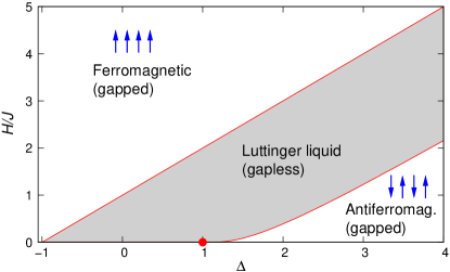
Figure 1: (Color online) Zero-temperature phase diagram of the spin-1/2 $XXZ$ chain in a magnetic field.

It is useful to recall the zero-temperature phase diagram of the model Eq. (4), see Fig. 1.JMcC72 ; AlMa95 ; CHP98 For $\Delta>1$ and small magnetic fields $H<H_{c1}$ there is long-range antiferromagnetic order along the $z$-direction in spin space. This state exhibits a gap in the excitation spectrum whose value at $H=0$ corresponds to $H_{c1}$. The value of the gap has been computed exactly via the Bethe ansatz.CG66 ; yang_yang_1966_3 In particular, it is exponentially small close to the Heisenberg point at $\Delta=1$ (marked by the dot in Fig. 1), which is characteristic for a Kosterlitz-Thouless transition.KT73 ; Kosterlitz For $\Delta<1$, one finds a gapless Luttinger-liquid state.Haldane This Luttinger-liquid state exists for $\left|\Delta\right|<1$, $H<H_{c2}$ and $\Delta>1$, $H_{c1}<H<H_{c2}$, with $H_{c2}=J\,(1+\Delta)$. Finally, for $H>H_{c2}$, the ground state is the ferromagnetically polarized state along the $z$-direction which exhibits again a gap. We anticipate that these different zero-temperature regions, in particular the quantum phase transitions at $H_{c1}$ and $H_{c2}$ will be reflected by the magnetocaloric properties at finite temperature.

II.1 Non-linear integral equations

In this section we recall the approach to the thermodynamics using the QTM technique and NLIEs.klu ; klu98 The equations look different for $\left|\Delta\right|<1$ and $\left|\Delta\right|>1$.

First we consider the case $\left|\Delta\right|<1$. One can represent the free energy of the system per lattice site in the following form:

$$f=e_{0}-T\int\limits_{-\infty}^{\infty}\frac{\ln\left[(1+a(x))(1+\overline{a}(x))\right]}{4\cosh\frac{\pi x}{2}}\,dx$$ (5)

(the constant $e_{0}$ is irrelevant in the present context). The auxiliary functions $a(x)$ and $\overline{a}(x)$ are found from the following system of integral equations

$$\ln a(x) = -\frac{J\sin\gamma}{T2\gamma}\frac{\pi}{\cosh\frac{\pi x}{2}}+\frac{\pi H}{2T\left(\pi-\gamma\right)}+\kappa*\ln(1+a)(x)-\kappa^{+}*\ln(1+\overline{a})(x)\,,$$ (6a)

$$\ln\overline{a}(x) = -\frac{J\sin\gamma}{T2\gamma}\frac{\pi}{\cosh\frac{\pi x}{2}}-\frac{\pi H}{2T\left(\pi-\gamma\right)}+\kappa*\ln(1+\overline{a})(x)-\kappa^{-}*\ln(1+a)(x)\,.$$ (6b)

Here $\gamma=\arccos\Delta$, the symbol $*$ denotes convolution $f*g(x)=\int_{-\infty}^{\infty}f(x-y)g(y)dy$ and the function $\kappa(x)$ is defined by

$$\kappa(x)=\frac{1}{2\pi}\int\limits_{-\infty}^{\infty}\frac{\sinh\left(\frac{\pi}{\gamma}-2\right)k}{2\cosh k\sinh\left(\frac{\pi}{\gamma}-1\right)k}e^{ikx}dk\,,\qquad\kappa^{\pm}(x)=\kappa(x\pm 2i)\,.$$ (7)

These equations are valid for $0<\Delta<1$. Results for negative $\Delta$ can be obtained by changing the sign of the coupling $J$.

For the case $\Delta>1$ the free energy has the form

$$f=e_{0}-\frac{T}{2}c\star\ln\left[(1+\mathfrak{b})(1+\bar{\mathfrak{b}})\right](0)=e_{0}-\frac{T}{2\pi}\int\limits_{-\pi/2}^{\pi/2}\,c(x)\ln\left[(1+\mathfrak{b}(x))(1+\bar{\mathfrak{b}}(x))\right]dx$$ (8)

with $f\star g(x)=\frac{1}{\pi}\int_{-\pi/2}^{\pi/2}dy\,f(x-y)g(y)$ denoting a convolution with modified integration limits and

$$c(x)=\sum_{k=-\infty}^{\infty}\frac{1}{\cosh(\eta k)}e^{i2kx}\,,$$ (9)

with $\Delta=\cosh\eta$. The auxiliary functions are solutions of the following integral equations

$$\ln\mathfrak{b}(x)= -\frac{J\sinh(\eta)}{2T}c(x)+\frac{H}{2T}+k\star\ln\left(1+\mathfrak{b}(x)\right)-k^{+}\star\ln\left(1+\bar{\mathfrak{b}}(x)\right)$$ (10a)

$$\ln\bar{\mathfrak{b}}(x)= -\frac{J\sinh(\eta)}{2T}c(x)-\frac{H}{2T}+k\star\ln\left(1+\bar{\mathfrak{b}}(x)\right)-k^{-}\star\ln\left(1+\mathfrak{b}(x)\right)$$ (10b)

with integration kernels

$$k(x)=\sum_{k=-\infty}^{\infty}\frac{e^{-\eta|k|}}{2\cosh(\eta k)}e^{i2kx}\,,\qquad k^{\pm}(x)=k(x\pm i\eta^{\mp})\,.$$ (11)

Results for $\Delta<-1$ can again be obtained by changing the sign of the coupling $J$.

The equations for the isotropic case $\Delta=1$ can be obtained by taking the limit $\gamma\rightarrow 0$ from the case $\left|\Delta\right|<1$ in (5) and (6) or from the case $\left|\Delta\right|>1$ by changing the spectral parameter $x=\tilde{x}\eta$ and taking the limit $\eta\rightarrow 0$ in (8) and (10).

Having all these exact expressions one can obtain any thermodynamic quantity of interest by iteration of the NLIE (6) (or (10)) and numerical integration of the expression for the free energy (5) (or (8)). Derivatives of the free energy with respect to $T$ and $H$ can also be calculated. One can avoid numerical differentiation by solving the associated integral equations for the differentiated auxiliary functions, e.g. $\partial_{H}\ln a(x)$. Note that derivatives of $\ln a(x)$ and $\ln\overline{a}(x)$ are treated as independent functions in these equations. As an example we will give the equations for the calculation of the magnetization per spin $M$ and the derivative of $M$ with respect to the temperature in the regime $\left|\Delta\right|<1$

$$M=T\int\limits_{-\infty}^{\infty}\frac{1}{4\cosh\frac{\pi x}{2}}\left(\frac{a(x)}{1+a(x)}\left[\partial_{H}\ln a(x)\right]+\frac{\overline{a}(x)}{1+\overline{a}(x)}\left[\partial_{H}\ln\overline{a}(x)\right]\right)dx\,.$$ (12)

The derivatives $\partial_{H}\ln a(x)$ and $\partial_{H}\ln\overline{a}(x)$ satisfy linear integral equations in which the auxiliary functions $a(x)$ and $\overline{a}(x)$ enter as external functions

$$\partial_{H}\ln a(x) = \frac{\pi}{2T\left(\pi-\gamma\right)}+\kappa*\frac{a}{1+a}\left[\partial_{H}\ln a\right](x)-\kappa*\frac{\overline{a}}{1+\overline{a}}\left[\partial_{H}\ln\overline{a}\right](x+2i)\,,$$ (13a)

$$\partial_{H}\ln\overline{a}(x) = -\frac{\pi}{2T\left(\pi-\gamma\right)}+\kappa*\frac{\overline{a}}{1+\overline{a}}\left[\partial_{H}\ln\overline{a}\right](x)-\kappa*\frac{a}{1+a}\left[\partial_{H}\ln a\right](x-2i)\,.$$ (13b)

To obtain the cooling rate $\Gamma_{H}$ we have to determine $\partial M/\partial T$. In order to achieve this we have to differentiate (12) with respect to $T$. However it has turned out that in the framework of NLIEs the resulting equations in general behave numerically better if the derivatives are taken with respect to the inverse temperature $\beta=1/T$ (we set $k_{B}=1$).

$$\left(\frac{\partial M}{\partial T}\right)_{H} =-\beta^{2}\left(\frac{\partial M}{\partial\beta}\right)_{H}=$$

$$\int\limits_{-\infty}^{\infty}\frac{1}{4\cosh\frac{\pi x}{2}}\left(\frac{a(x)}{1+a(x)}\left[\partial_{H}\ln a(x)\right]+\frac{\overline{a}(x)}{1+\overline{a}(x)}\left[\partial_{H}\ln\overline{a}(x)\right]\right)dx$$

$$-\beta\int\limits_{-\infty}^{\infty}\frac{1}{4\cosh\frac{\pi x}{2}}\left[\left(\frac{a(x)}{1+a(x)}-\left(\frac{a(x)}{1+a(x)}\right)^{2}\right)\left[\partial_{\beta}\ln a(x)\right]\left[\partial_{H}\ln a(x)\right]+\frac{a(x)}{1+a(x)}\left[\partial_{\beta}\partial_{H}\ln a(x)\right]\right.$$

$$\quad\quad\quad\left.+\left(\frac{\overline{a}(x)}{1+\overline{a}(x)}-\left(\frac{\overline{a}(x)}{1+\overline{a}(x)}\right)^{2}\right)\left[\partial_{\beta}\ln\overline{a}(x)\right]\left[\partial_{H}\ln\overline{a}(x)\right]+\frac{\overline{a}(x)}{1+\overline{a}(x)}\left[\partial_{\beta}\partial_{H}\ln\overline{a}(x)\right]\right]dx\,.$$ (14)

Here four new functions $\partial_{\beta}\ln a(x)$, $\partial_{\beta}\partial_{H}\ln a(x)$ and their $\overline{a}$ counterparts occur. The corresponding linear integral equations read

$$\partial_{\beta}\ln a(x) = -\frac{J\sin\gamma}{2\gamma}\frac{\pi}{\cosh\frac{\pi x}{2}}+\frac{\pi H}{2\left(\pi-\gamma\right)}+\kappa*\frac{a}{1+a}\left[\partial_{\beta}\ln a\right](x)-\kappa^{+}*\frac{\overline{a}}{1+\overline{a}}\left[\partial_{\beta}\ln\overline{a}\right](x)\,,$$ (15a)

$$\partial_{\beta}\ln\overline{a}(x) = -\frac{J\sin\gamma}{2\gamma}\frac{\pi}{\cosh\frac{\pi x}{2}}-\frac{\pi H}{2\left(\pi-\gamma\right)}+\kappa*\frac{\overline{a}}{1+\overline{a}}\left[\partial_{\beta}\ln\overline{a}\right](x)-\kappa^{-}*\frac{a}{1+a}\left[\partial_{\beta}\ln a\right](x)\,,$$ (15b)

and

$$\partial_{\beta}\partial_{H}\ln a(x)= \frac{\pi}{2\left(\pi-\gamma\right)}+\kappa*\left[\left(\frac{a}{1+a}-\left(\frac{a}{1+a}\right)^{2}\right)\left[\partial_{\beta}\ln a\right]\left[\partial_{H}\ln a\right]+\frac{a}{1+a}\left[\partial_{\beta}\partial_{H}\ln a\right]\right](x)$$

$$\quad-\kappa^{+}*\left[\left(\frac{\overline{a}}{1+\overline{a}}-\left(\frac{\overline{a}}{1+\overline{a}}\right)^{2}\right)\left[\partial_{\beta}\ln\overline{a}\right]\left[\partial_{H}\ln\overline{a}\right]+\frac{\overline{a}}{1+\overline{a}}\left[\partial_{\beta}\partial_{H}\ln\overline{a}\right]\right](x)\,,$$ (16a)

$$\partial_{\beta}\partial_{H}\ln\overline{a}(x)= -\frac{\pi}{2\left(\pi-\gamma\right)}+\kappa*\left[\left(\frac{\overline{a}}{1+\overline{a}}-\left(\frac{\overline{a}}{1+\overline{a}}\right)^{2}\right)\left[\partial_{\beta}\ln\overline{a}\right]\left[\partial_{H}\ln\overline{a}\right]+\frac{\overline{a}}{1+\overline{a}}\left[\partial_{\beta}\partial_{H}\ln\overline{a}\right]\right](x)$$

$$\quad-\kappa^{-}*\left[\left(\frac{a}{1+a}-\left(\frac{a}{1+a}\right)^{2}\right)\left[\partial_{\beta}\ln a\right]\left[\partial_{H}\ln a\right]+\frac{a}{1+a}\left[\partial_{\beta}\partial_{H}\ln a\right]\right](x)\,.$$ (16b)

Note that the functions $\partial_{\beta}\ln a(x)$ and $\partial_{\beta}\ln\overline{a}(x)$ already allow the calculation of the entropy per spin

$$S=\int\limits_{-\infty}^{\infty}\frac{\ln\left[(1+a(x))(1+\overline{a}(x))\right]}{4\cosh\frac{\pi x}{2}}\,dx-\frac{1}{T}\int\limits_{-\infty}^{\infty}\frac{1}{4\cosh\frac{\pi x}{2}}\left(\frac{a(x)}{1+a(x)}\left[\partial_{\beta}\ln a(x)\right]+\frac{\overline{a}(x)}{1+\overline{a}(x)}\left[\partial_{\beta}\ln\overline{a}(x)\right]\right)dx\,.$$ (17)

For the calculation of the cooling rate $\Gamma_{H}$ the specific heat is needed in addition to the mixed derivative $\partial M/\partial T$. It can be obtained by differentiating (17) with respect to $\beta$ and dividing by $-T$. In the resulting equation another pair of functions $\partial_{\beta}^{2}\ln a(x)$, $\partial_{\beta}^{2}\ln\overline{a}(x)$ occurs, where the corresponding integral equations are derived by differentiating (15) again with respect to $\beta$ in close analogy to (16).

II.2 Comparison with numerical results

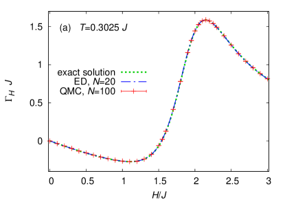
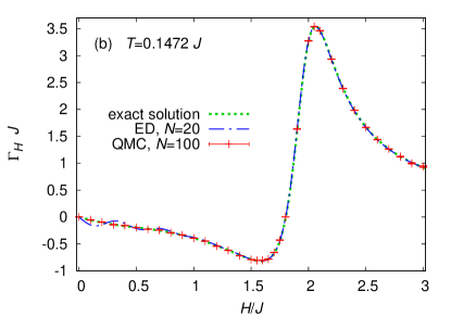
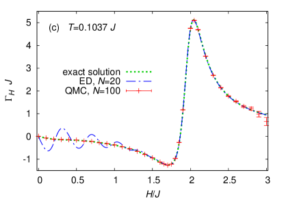
Figure 2: (Color online) Cooling rate $\Gamma_{H}$ for the Heisenberg chain ($\Delta=1$). Shown are exact diagonalization (ED) for $N=20$ sites, Quantum Monte Carlo (QMC) for $N=100$ sites and the exact solution for the infinite system. The different panels are for $T/J=0.3025$ (a), $0.1472$ (b), and $0.1037$ (c).

First, we present a comparison with numerical methods, namely exact diagonalization (ED) and Quantum Monte Carlo (QMC). On the one hand, this comparison will serve as a cross-check of our results. On the other hand, we can use the exact results to assess the performance of the numerical methods.

The quantities appearing on the r.h.s. of Eq. (2) can be expressed as follows:

$$C_{H} = \frac{\beta^{2}}{N}\,\left(\left\langle\mathcal{H}^{2}\right\rangle-\left\langle\mathcal{H}\right\rangle^{2}\right)\,,$$ (18)

$$\left(\frac{\partial M}{\partial T}\right)_{H} = \frac{\beta^{2}}{N}\,\left(\left\langle M\,\mathcal{H}\right\rangle-\left\langle M\right\rangle\left\langle\mathcal{H}\right\rangle\right)\,,$$ (19)

where $\langle\cdot\rangle$ is the expectation value at a fixed temperature $T$ and magnetic field $H$. Here we have chosen a normalization per spin which drops out when taking the ratio in Eq. (2). Eq. (18) is well known and Eq. (19) is valid for any Hamiltonian conserving magnetization, i.e., $\left[M,\mathcal{H}\right]=0$.

One can write down spectral representations for the correlation functions in Eqs. (18) and (19) which can be evaluated by ED. These correlation functions can also be evaluated with QMC. The QMC simulations to be reported below have been carried out with the ALPSalps1 ; alps2 directed loop applicationalps-sse in the stochastic series expansion framework.Sandvik The specific heat Eq. (18) is measured using an improved estimator which involves the fluctuations of the expansion order.SSS The correlation function Eq. (19) can be measured in a similar manner. Note that it is crucial to choose an appropriate pseudo random-number generator in order to obtain correct results. We have used the “Mersenne Twister”.MTrng In our QMC simulations we have performed $4\cdot 10^{5}$ thermalization steps and then collected data during a number of sweeps ranging between $2\cdot 10^{7}$ and $3.3\cdot 10^{10}$.

Fig. 2 shows a comparison of $\Gamma_{H}$ between the exact solution for $N=\infty$, ED for $N=20$, and QMC for $N=100$ at three temperatures which have been chosen to correspond to the experiments of Ref. Tsui, . The ED curves exhibit some wiggles at small magnetic fields and temperatures which reflect the fact that the system contains only $N=20$ sites. In this regime, the QMC results for $N=100$ are indistinguishable from the exact solution for $N=\infty$ on the scale of Fig. 2. On the other hand, the QMC results are subject to big error bars at high fields and low temperatures despite the fact that we have invested substantial amounts of CPU time into these data points. To some extent, this is related to performance problems of the algorithm in a magnetic field.Sandvik However, the main reason is that $\Gamma_{H}$ is given by the ratio of two quantities (see Eq. (2)) which are both exponentially small in $T$ for $H>H_{c2}=2\,J$. Indeed, even with a large number of sweeps, it is difficult to determine the ratio of two very small quantities accurately by QMC. Conversely, the existence of a gap improves finite-size convergence such that ED works particularly well in the high-field regime.

The overall good agreement between all three methods serves as a consistency check for each of them. Furthermore, we see that we can get extremely accurate numerical results by combining QMC for $H\lesssim H_{c2}$ and ED for $H\gtrsim H_{c2}$ ($H_{c2}=2\,J$ in the present case).

II.3 Effects of anisotropy $\Delta$

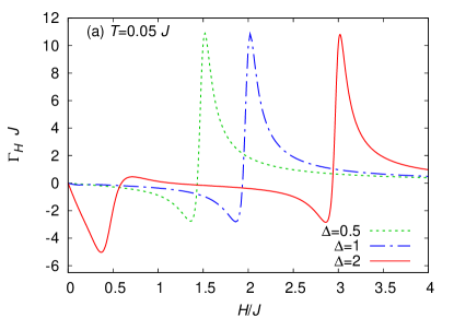
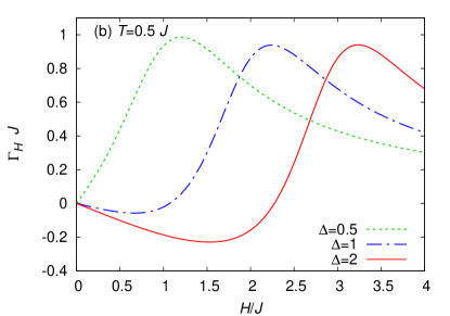
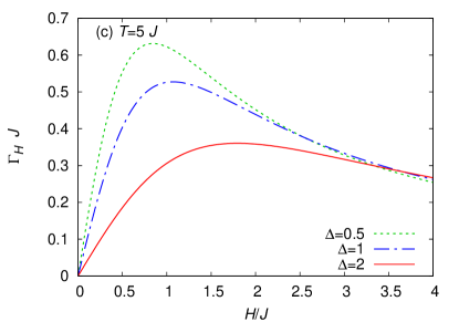
Figure 3: (Color online) Cooling rate $\Gamma_{H}$ for different values of the anisotropy. Shown is the exact solution for the infinite system. The different panels are for $T/J=0.05$ (a), $0.5$ (b), and $5$ (c).

Next, we discuss the effects of exchange anisotropy on the cooling rate. Fig. 3 shows results for three selected values $\Delta=0.5$, $1$, and $2$. Recall from Fig. 1 that, at $\Delta=0.5$, one crosses just one quantum phase transition at $H_{c2}=1.5\,J$, the curves for $\Delta=1$ in Fig. 3 start from the special Heisenberg point at $H=0$ and cross the transition to saturation at $H_{c2}=2\,J$, and the curves at $\Delta=2$ cut two quantum phase transitions, namely $H_{c1}\approx 0.39\,J$ and $H_{c2}=3\,J$. For $T=0.05\,J$, the quantum phase transitions at $H_{c2}$ and for $\Delta=2$ at $H_{c1}$ are signaled by sign changes of the cooling rate $\Gamma_{H}$ from negative to positive values upon increasing field, see Fig. 3(a). Note that these zeros shift away from the position of the zero-temperature phase transitions with increasing temperature, as is evident in particular if one takes into account the additional data for $\Delta=1$ shown in Fig. 2. Finally, there is a small structure at low magnetic fields in the $\Delta=1$ curves of Figs. 2(c) and 3(a) which reflects the singular nature of the Heisenberg point $(\Delta=1,H=0)$.

At the isotropic point of the antiferromagnetic $XXZ$ chain, the quantity $\Gamma_{H}/H$ shows singular behavior for $T\to 0$ if $H<T$. In fact, in the limit of $H\to 0$ the ratio reduces to the temperature derivative of the zero-field susceptibility $\chi(T)$

$$\lim_{H\to 0}\frac{\Gamma_{H}(T)}{H}=-\frac{1}{C_{H}}\left(\frac{\partial\chi}{\partial T}\right)_{H}\,,$$ (20)

which is known to show singular behavior. For $\Delta=1$ this function diverges like $\mbox{const.}\times[T\ln(T_{0}/T)]^{-2}$ where $T_{0}$ is a (non-universal) constant.Lukyanov For $\Delta<1$ the function (20) diverges like $\mbox{const.}\times T^{4K-6}$ with Tomonaga-Luttinger parameter $K=\pi/(\pi-\gamma)>1$.Sirker For $\Delta>1$ a divergent behavior like $\mbox{const.}/T$ is observed. The strongest divergence is hence exhibited for $\Delta=1$. For finite magnetic field $H$ we see a non-divergent behavior for $T\rightarrow 0$.

With increasing temperature, all features become broader. Note that the temperature $T=0.5\,J$ shown in Fig. 3(b) is higher than the value of $H_{c1}$ at $\Delta=2$ which explains why the sign change around $H_{c1}$ in the $\Delta=2$ curve disappears for $T=0.5\,J$. For the even higher temperature $T=5\,J$ shown in Fig. 3(c), the cooling rate $\Gamma_{H}$ is positive for all $H>0$ (the zero at $H=0$ is enforced by the symmetry under $H\to-H$). Note that $T=5\,J$ is bigger than $H_{c2}$ itself for all cases shown in Fig. 3(c) which explains why all features are washed out at this temperature.

II.4 The case of infinitely large anisotropy: cooling rate for the Ising chain

The case of infinitely large anisotropy ($\Delta\to\infty$ at $J_{I}=J\Delta=\mbox{const.}$) corresponds to the Ising model with Hamiltonian

$$\mathcal{H}=J\sum_{i=1}^{N}s_{i}s_{i+1}-H\sum_{i=1}^{N}s_{i}\,,$$ (21)

where the classical variables $s_{i}$ take values $\pm 1/2$ and for simplicity reasons we drop the subscript of the coupling $J_{I}$ in this section. It is well known that the Ising chain can be solved exactly and completely analytically by the transfer-matrix method (see for example Refs. Huang, ; bax, ) and even $\left(\partial M/\partial T\right)_{H}$ was investigated recently.Sznajd08 However, we are not aware of explicit results for the entropy $S$ and normalized cooling rate $\Gamma_{H}$ of the Ising chain and therefore present them here.

We start from the free energy per lattice site of the Ising chain:

$$f=-\frac{1}{\beta}\ln\left(e^{-\beta J/4}\left(\cosh(\beta H/2)+\sqrt{\sinh^{2}(\beta H/2)+e^{\beta J}}\right)\right)\,.$$ (22)

From this expression one can easily obtain simple analytic expressions for all thermodynamic functions of the system. In particular one obtains for the entropy per spin and the normalized cooling rate:

$$S = -\left(\frac{\partial f}{\partial T}\right)_{H}=\ln\left(e^{-\beta J/4}\left(c+Q\right)\right)-\frac{-J/4(c+Q)+sH/2+\frac{sH/2+Je^{\beta J}}{Q}}{T(c+Q)}\,,$$ (23)

$$\Gamma_{H} = \frac{1}{T}\left(\frac{\partial T}{\partial H}\right)_{S}=-\frac{\frac{\partial^{2}f}{\partial T\partial H}}{T\frac{\partial^{2}f}{\partial T^{2}}}=\frac{1/2(cH/2-sJ/2)(c+Q)^{2}}{1/2J^{2}s^{2}Q+1/4J^{2}c(s^{2}+Q^{2})+H/2(cH/2-Js)(c+Q)^{2}}\,,$$ (24)

where

$$c=\cosh(\beta H/2)\,,\qquad s=\sinh(\beta H/2)\,,\qquad Q=\sqrt{\sinh^{2}(\beta H/2)+e^{\beta J}}\,.$$ (25)

The $T=0$ limit of the entropy (23) is generically $S=0$, except for $H=\pm J$, where one finds $S=\ln\left(\frac{1+\sqrt{5}}{2}\right)=0.4812\ldots$ (see also Ref. MeYa78, ). This reflects the macroscopic ground-state degeneracy of the Ising model at the saturation field $H_{c}=J$.Bonner1962 Remarkably, the above transfer-matrix solution is closely related to the hard-dimer description of certain highly frustrated one-dimensional quantum antiferromagnets.zhhon ; Derzhko07 ; DeRi04 ; ZhiT04 ; ZhiT05

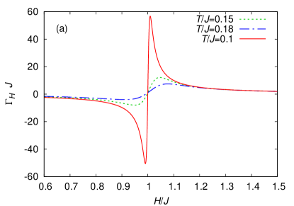
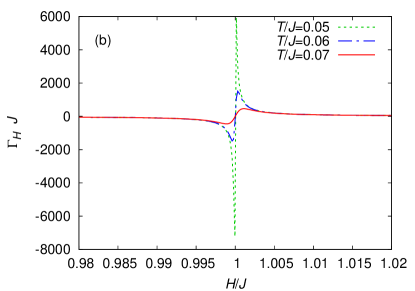
Figure 4: (Color online) Cooling rate $\Gamma_{H}$ of the Ising model ($\Delta\to\infty$ limit of the $XXZ$ model). Shown is the exact solution for the infinite system. The different panels show the cooling rate for a wider range of temperatures (a) and the behavior at low temperatures in the vicinity of the critical point (b).

Fig. 4 shows the cooling rate dependence on the magnetic field for the Ising chain obtained from the exact solution. The main difference from the $XXZ$ case are the very sharp and pronounced positive and negative peaks at the critical value of the magnetic field. The magnitude of these peaks grows rapidly with decreasing temperature. This behavior is a direct consequence of the anomalous zero-temperature entropy of the Ising chain at $H=J$.Bonner1962

A bit further away from the QCP at $H_{c}=J$, we can make contact with the argumentation of Ref. Garst, . The Grüneisen ratio, which in our case is the cooling rate $\Gamma_{H}$, shows divergent behavior close to the QCP at $H_{c}$ and changes sign when the magnetic field crosses it. For $H\neq H_{c}$, the divergent behavior obeys the universal scaling lawZhu ; Garst

$$\Gamma_{H}\left(T\rightarrow 0,H\right)=-G_{H}\frac{1}{H-H_{c}},$$ (26)

where $G_{H}$ is a universal amplitude. Detailed analysis of the Ising case yields the exact analytic form of the cooling rate at extremely low temperatures, $\Gamma_{H}^{\rm Ising}\left(T\rightarrow 0\right)=\frac{1}{H-J}$ for $T\ll\left|H-J\right|$, i.e., the value $G_{H}=-1$ expected for a $\mathbb{Z}_{2}$-symmetry in one dimension.Garst ; zhhon

II.5 Entropy

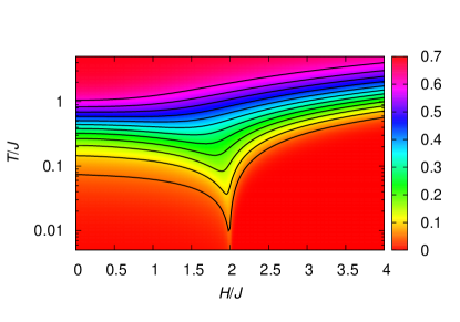
Figure 5: (Color online) Entropy per spin $S(H,T)$ for $\Delta=1$. The isentropes are for $S=0.05,0.1,\ldots,0.6$.

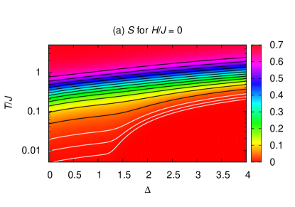
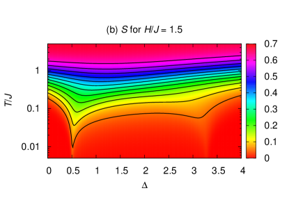
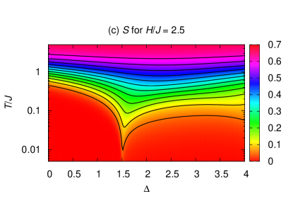
Figure 6: (Color online) Entropy per spin $S(\Delta,T)$ for different values of $H=0$ (a), $1.5\,J$ (b), and $2.5\,J$ (c). The black lines are the isentropes for $S=0.05,0.1,\ldots,0.6$. Panel (a) contains three additional isentropes with $S=0.005$, $0.01$, and $0.02$ which are shown by white lines.

Finally, we take a look at the entropy $S$. As far as we are aware, there has been only one previous attempt of an exact computationBonner1977 of the entropy and accordingly the isentropes of the $XXZ$ chain in a magnetic field. Inspection of the critical fields $H_{c1}$ and $H_{c2}$ indicates that the result of Ref. Bonner1977, corresponds to an anisotropy $\Delta\approx 4.75$. The main technical difference between Ref. Bonner1977, and the present work is that Ref. Bonner1977, worked with an infinite hierarchy of equations for $\Delta>1$ which need to be truncated while we have a closed finite set of equations for all values of $\Delta$. In the case $|\Delta|<1$ the structure of the NLIE (6) is independent of $\Delta$ in contrast to the usual TBA equations, which allows to easily calculate the entropy as a function of the anisotropy.

Fig. 5 shows the entropy and the isentropes for the spin-1/2 Heisenberg chain in the $H$-$T$ plane. This result agrees with previous ED for $N=20$ sites.zhhon However, the ED results of Ref. zhhon, suffered from finite-size effects, in particular for low temperatures and $H<H_{c2}=2\,J$. By contrast, Fig. 5 shows results for the thermodynamic limit. Fig. 6 shows a similar plot of the entropy and isentropes with varying anisotropy $\Delta$ but now at a fixed magnetic field $H$. The quantum phase transitions at $H_{c1}$ and $H_{c2}$ are reflected in Figs. 5 and 6 by minima of the isentropes as a function of $H$ or $\Delta$, or equivalently maxima of the entropy at a low but constant temperature. The only exception is Fig. 6(a) where one observes no such clear signature of the Kosterlitz-Thouless transition at $\Delta=1$ for $H=0$. Before we discuss this case in more detail, it is useful to examine the low-temperature asymptotics of the entropy $S(T)$ at otherwise fixed parameters $H$ and $\Delta$.

Between the two quantum critical points, that is for $H_{c1}<H<H_{c2}$, the low-energy theory is a Luttinger liquid (compare remarks at the beginning of Sec. II). It is well known that the specific heat $C$ of a Luttinger liquid is linear in $T$.Giamarchi Due to the relation $C=T\,(\partial\,S/\partial T)$ (see, e.g., Ref. rev2, ) and because of $S(T=0)=0$, the entropy of a Luttinger liquid is identical to its specific heat and in particular also linear

$$S=\frac{\pi}{3\,v}\,T\quad\mbox{for }H_{c1}<H<H_{c2}\,,$$ (27)

where $v$ is the velocity of the excitations.

The cases $H=H_{c1}$ and $H_{c2}$ are instances of a quantum phase transition in one dimension which preserves a $U(1)$-symmetry. In this case, the universal low-temperature asymptotics is predicted to follow a square rootBonner1972 ; zhhon ; Zhu ; Garst

$$S\propto\sqrt{\frac{T}{J}}\quad\mbox{for }H=H_{c1}\mbox{ or }H_{c2}\,.$$ (28)

Finally, in the gapped cases $0\leq H<H_{c1}$ or $H>H_{c2}$, we expect activated behavior

$$S\propto\exp(-G/T)\,,$$ (29)

where $G$ is the gap in the excitation spectrum. Closer inspection of the data shown in Figs. 5 and 6 indeed verifies Eqs. (27), (28), or (29), respectively. Note that while the asymptotic behavior is $S\to 0$ for $T\to 0$ in all three cases, the decay is slowest exactly at the quantum phase transition, see Eq. (28). This naturally yields a maximum of the entropy $S$ if the quantum phase transition is crossed by varying the parameters $H$ or $\Delta$ at a fixed temperature $T>0$.

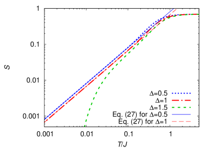
Figure 7: (Color online) Entropy per spin $S$ of the $XXZ$ chain at $H=0$ for $\Delta=0.5$, $1$, and $1.5$. For $\Delta=0.5$ and $1$ we also show the Luttinger-liquid expression Eq. (27) with the velocity $v$ given by Eq. (30).

The case $\Delta=1$, $H=0$ is an exception to this general scenario. To first approximation, this point behaves like a Luttinger liquid. The fact that one is at a quantum critical point with marginally irrelevant operators gives rise to higher-order logarithmic corrections in the free energy and specific heat.klu98 ; klu00 Consequently, one also expects just higher-order logarithmic corrections to the entropy. To test this scenario, we can use the fact that at $H=0$ the velocity $v$ which enters (27) is known exactly (see, e.g., Refs. Haldane, ; Giamarchi, ):

$$v=\frac{\pi\,\sin{\gamma}}{2\,\gamma}\,J$$ (30)

with $\Delta=\cos\gamma$ as above. Fig. 7 shows that insertion of these values of $v$ into the Luttinger-liquid expression Eq. (27) yields indeed the correct low-temperature asymptotics of the entropy per spin at $H=0$ not only for $\Delta=0.5$ but also for $\Delta=1$. In fact, the higher-order logarithmic corrections to the Luttinger liquid asymptotics (27) which are expected at $\Delta=1$ and $H=0$ are so small that they have no visible effect.

A gap $G$ opens for $\Delta>1$ at $H=0$, but because the phase transition is a Kosterlitz-Thouless transition,KT73 ; Kosterlitz this gap is exponentially small close to $\Delta=1$.CG66 ; yang_yang_1966_3 Accordingly, close to $\Delta=1$ one has to go to very low temperatures in order to observe the crossover from (27) to (29). This is illustrated by the $\Delta=1.5$ curve in Fig. 7. In the concrete case $\Delta=1.5$, the value of the gap is $G\approx 0.087\,J$. Accordingly, the exponential decay (29) can be observed only for temperatures $T\lesssim 0.05\,J$ while at higher temperatures the behavior of $S(T)$ remains approximately linear.

The combined effect of all these observations is that just a small kink develops in the low-temperature isentropes of Fig. 6(a) whose position shifts very slowly to the quantum critical point $\Delta=1$ for $T\to 0$.

III Conclusion and Perspectives

Motivated by recent measurements of the magnetic cooling rate in a spin-1/2 Heisenberg chain compound,Tsui we have presented an exact computation of the entropy and the magnetic cooling rate of the antiferromagnetic spin-1/2 $XXZ$ chain in the thermodynamic limit $N\to\infty$. Furthermore, we have performed complementary numerical computations for the cooling rate of finite Heisenberg chains, namely exact diagonalization (ED) for small systems and QMC simulations for somewhat longer chains. We have demonstrated that we can obtain excellent approximations to the exact result with a combination of both numerical methods. On the one hand, this serves as a consistency check of our computations. On the other hand, we are now in a position to apply a combination of ED and QMC to some sign-free situations, like the spin-1/2 Heisenberg model on the square and simple cubic lattices where the exact methods are no longer applicable.

We have used the exact result for the entropy to illustrate that field-induced quantum phase transitions give rise to maxima of the low-temperature entropy, or equivalently minima of the isentropes. This leads to cooling during adiabatic (de)magnetization processes where the lowest temperature is reached close to the quantum phase transition. As a consequence, we find a zero for the magnetic cooling rate at the phase transition and large positive (negative) values of the normalized cooling rate (2) for magnetic fields slightly above (below) the critical field.

The low-temperature asymptotics of the entropy $S$ is exponentially activated in the gapped phases, linear in $T$ in the gapless Luttinger liquid regions, and follows the square-root behavior (28) at the field-induced quantum phase transitions. These asymptotic forms of $S(T)$ are expected to be universal for field-induced phase transitions in one-dimensional systems with $U(1)$-symmetry,Bonner1972 ; zhhon ; Zhu ; Garst but can be particularly clearly verified with the aid of an exact solution.

The general features of the entropy should not depend on the specific choice of the magnetic field $H$ as control parameter and indeed similar behavior is found as a function of the exchange anisotropy $\Delta$. An exception is just the quantum phase transition at $H=0$, $\Delta=1$ with $\Delta$ as a control parameter. Because this is a Kosterlitz-Thouless transition, only weak signatures are observed in the finite-temperature entropy.

Finally, closed-form expressions were derived in the Ising limit using the transfer matrix method.Huang ; bax We have observed remarkably large magnetic cooling rates close to the field-induced critical point of the Ising chain. In fact, the transfer-matrix solution is closely related to a low-energy description of highly frustrated one-dimensional quantum antiferromagnets,zhhon ; Derzhko07 ; DeRi04 ; ZhiT04 ; ZhiT05 where enhanced cooling rates are observed as well.

- (1) E. Warburg, Ann. Phys. Chem. 13, 141 (1881).
- (2) K. A. Gschneider, Jr., V. K. Pecharsky, and A. O. Tsokol, Rep. Prog. Phys. 68, 1479 (2005).
- (3) A. M. Tishin and Y. I. Spichkin, The Magnetocaloric Effect and its Applications, (Institute of Physics Publishing, Bristol, 2003).
- (4) D. P. MacDougall and W. F. Giauque, Phys. Rev. 43, 768 (1933).
- (5) A. S. Oja and O. V. Lounasmaa, Rev. Mod. Phys. 69, 1 (1997).
- (6) T. Knuuttila, Ph.D. thesis, Helsinki University of Technology, 2000.
- (7) P. Strehlow, H. Nuzha, and E. Bork, J. Low Temp. Phys. 147, 81 (2007).
- (8) A. M. Tishin, Magnetocaloric effect in the vicinity of phase transitions, in Handbook of Magnetic Materials, edited by K. H. J. Buschow (Elsevier, Amsterdam, 1999) Vol. 12.
- (9) J. C. Bonner and J. F. Nagle, Phys. Rev. A 5, 2293 (1972).
- (10) J. C. Bonner and M. E. Fisher, Proc. Phys. Soc. 80, 508 (1962).
- (11) J. C. Bonner and J. D. Johnson, Physica 86-88B, 653 (1977).
- (12) M. E. Zhitomirsky and A. Honecker, J. Stat. Mech.: Theor. Exp. P07012 (2004).
- (13) A. S. Boyarchenkov, I. G. Bostrem, and A. S. Ovchinnikov, Phys. Rev. B 76, 224410 (2007).
- (14) A. Honecker and S. Wessel, Condensed Matter Physics 12, 399 (2009).
- (15) Y. Tsui, B. Wolf, D. Jaiswal-Nagar, U. Tutsch, A. Honecker, K. Remović-Langer, G. Hofmann, A. Prokofiev, W. Assmus, G. Donath, and M. Lang, in preparation.
- (16) L. Zhu, M. Garst, A. Rosch, and Q. Si, Phys. Rev. Lett. 91, 066404 (2003).
- (17) M. Garst and A. Rosch, Phys. Rev. B 72, 205129 (2005).
- (18) M. E. Zhitomirsky, Phys. Rev. B 67, 104421 (2003).
- (19) S. S. Sosin, L. A. Prozorova, A. I. Smirnov, A. I. Golov, I. B. Berkutov, O. A. Petrenko, G. Balakrishnan, and M. E. Zhitomirsky, Phys. Rev. B 71, 094413 (2005).
- (20) O. Derzhko and J. Richter, Eur. Phys. J. B 52, 23 (2006).
- (21) L. Čanová, J. Strečka, and M. Jaščur, J. Phys.: Condens. Matter 18, 4967 (2006).
- (22) O. Derzhko, J. Richter, A. Honecker, and H.-J. Schmidt, Low Temp. Phys. 33, 745 (2007).
- (23) M. S. S. Pereira, F. A. B. F. de Moura, and M. L. Lyra, Phys. Rev. B 79, 054427 (2009).
- (24) L. Čanová, J. Strečka, and T. Lučivjanský, Condensed Matter Physics 12, 353 (2009).
- (25) A. Honecker and S. Wessel, Physica B 378-380, 1098 (2006).
- (26) B. Schmidt, P. Thalmeier, and N. Shannon, Phys. Rev. B 76, 125113 (2007).
- (27) M. Gaudin, Phys. Rev. Lett. 26, 1301 (1971).
- (28) M. Takahashi, Thermodynamics of One-dimensional Solvable Models, (Cambridge, Cambridge University Press, 1999).
- (29) A. Klümper, Eur. J. Phys. B 5, 677 (1998).
- (30) A. Klümper and D. C. Johnston, Phys. Rev. Lett. 84, 4701 (2000).
- (31) A. Klümper, Lect. Notes Phys. 645, 349 (2004).
- (32) J. D. Johnson and B. M. McCoy, Phys. Rev. A 6, 1613 (1972).
- (33) F. C. Alcaraz and A. L. Malvezzi, J. Phys. A 28, 1521 (1995).
- (34) D. C. Cabra, A. Honecker, and P. Pujol, Phys. Rev. B 58, 6241 (1998).
- (35) J. des Cloizeaux and M. Gaudin, J. Math. Phys. 7, 1384 (1966).
- (36) C. N. Yang and C. P. Yang, Phys. Rev. 151, 258 (1966).
- (37) J. M. Kosterlitz and D. J. Thouless, J. Phys. C 6, 1181 (1973).
- (38) J. M. Kosterlitz, J. Phys. C 7, 1046 (1974).
- (39) F. D. M. Haldane, Phys. Rev. Lett. 45, 1358 (1980).
- (40) M. Troyer, B. Ammon, and E. Heeb, Lecture Notes in Computer Science 1505, 191 (1998).
- (41) A. F. Albuquerque, F. Alet, P. Corboz, P. Dayal, A. Feiguin, S. Fuchs, L. Gamper, E. Gull, S. Gürtler, A. Honecker, R. Igarashi, M. Körner, A. Kozhevnikov, A. Läuchli, S. R. Manmana, M. Matsumoto, I. P. McCulloch, F. Michel, R. M. Noack, G. Pawłowski, L. Pollet, T. Pruschke, U. Schollwöck, S. Todo, S. Trebst, M. Troyer, P. Werner, and S. Wessel, J. Magn. Magn. Mater. 310, 1187 (2007).
- (42) F. Alet, S. Wessel, and M. Troyer, Phys. Rev. E 71, 036706 (2005).
- (43) O. F. Syljuåsen and A. W. Sandvik, Phys. Rev. E 66, 046701 (2002).
- (44) P. Sengupta, A. W. Sandvik, and R. R. P. Singh, Phys. Rev. B 68, 094423 (2003).
- (45) M. Matsumoto and T. Nishimura, ACM TOMACS 8, 3 (1998).
- (46) S. Lukyanov, Nucl. Phys. B 522, 533 (1998).
- (47) J. Sirker and M. Bortz, J. Stat. Mech.: Theor. Exp. P01007 (2006).
- (48) K. Huang, Statistical Mechanics, (John Wiley & Sons, New York, 1963).
- (49) R. Baxter, Exactly Solved Models in Statistical Mechanics, (Academic Press, New York, 1982).
- (50) J. Sznajd, Phys. Rev. B 78, 214411 (2008).
- (51) B. D. Metcalf and C. P. Yang, Phys. Rev. B 18, 2304 (1978).
- (52) O. Derzhko and J. Richter, Phys. Rev. B 70, 104415 (2004).
- (53) M. E. Zhitomirsky and H. Tsunetsugu, Phys. Rev. B 70, 100403(R) (2004).
- (54) M. E. Zhitomirsky and H. Tsunetsugu, Progr. Theor. Phys. Suppl. 160, 361 (2005).
- (55) T. Giamarchi, Quantum Physics in One Dimension, (Clarendon Press, Oxford, 2004).