Gravitational energy as dark energy: Towards concordance cosmology without Lambda

Abstract

I briefly outline a new physical interpretation to the average cosmological parameters for an inhomogeneous universe with backreaction. The variance in local geometry and gravitational energy between ideal isotropic observers in bound structures and isotropic observers at the volume average location in voids plays a crucial role. Fits of a model universe to observational data suggest the possibility of a new concordance cosmology, in which dark energy is revealed as a mis-identification of gravitational energy gradients that become important when voids grow at late epochs.

1 Introduction

The last decade has seen a shift in our understanding of the expansion history of the universe, on account of precision measurements in observational cosmology. The current prevailing view, based on model universes which assume an exactly homogeneous and isotropic background geometry for the universe, is that the universe is undergoing a period of accelerating expansion, which began at relatively low redshifts. The cause of this acceleration – which in the standard framework would be due to some smooth fluidlike dark energy component that violates the strong energy condition – is widely viewed as one of the biggest challenges both for cosmology and fundamental physics. The simplest model for dark energy – a cosmological constant, $\Lambda$ – is consistent with many key observations, including in particular type Ia supernovae (SneIa) luminosity distances, the spectrum of cosmic microwave background (CMB) anisotropies, and the echo of the baryon acoustic oscillation (BAO) scale in the primordial plasma as reflected statistically in galaxy clustering.

Although the standard Lambda Cold Dark Matter ($\Lambda$CDM) model provides a good fit to many tests, there are tensions between some tests, and also a number of puzzles and anomalies. Furthermore, theoretically the existence of a cosmological constant begs the cosmic coincidence question: why does the cosmological constant have a precise very tiny value such that the universe only began accelerating at recent epochs, making the matter density parameter, $\Omega_{\lower 2.0pt\hbox{$\scriptstyle M0$}}$, and cosmological constant density parameter, $\Omega_{\lower 2.0pt\hbox{$\scriptstyle\Lambda 0$}}$, of similar order today?

At the same time as the majority of cosmologists have been pursuing ideas related to a fluidlike dark energy, or modifications of general relativity, while retaining homogeneous isotropic backgrounds, a small but growing number of cosmologists have questioned whether the the expansion history of the universe may be understood in terms of the growing inhomogeneous structure in recent epochs. (See, e.g., Célérier (2007) for a review.) After all, at the present epoch the universe is only statistically homogeneous once one samples on scales of 150–300 Mpc. Below such scales it displays a web–like structure, dominated in volume by voids. Some 40%–50% of the volume of the present epoch universe is in voids of 30$h^{-1}$ Mpc (Hoyle & Vogeley 2002, 2004), where $h$ is the dimensionless parameter related to the Hubble constant by $H_{\lower 2.0pt\hbox{$\scriptstyle 0$}}=100h\,\hbox{km}\;\,\hbox{sec}^{-1}\,\hbox{Mpc}^{-1}$. Once one also accounts for numerous minivoids, and perhaps also a few larger voids, then it appears that the present epoch universe is void-dominated. Clusters of galaxies are spread in sheets that surround these voids, and thin filaments that thread them.

One particular consequence of a matter distribution that is only statistically homogeneous, rather than exactly homogeneous, is that when the Einstein equations are averaged they do not evolve as a smooth Friedmann–Lemaître–Robertson–Walker (FLRW) geometry. Instead the Friedmann equations is supplemented by additional backreaction terms (Buchert, 2000). Whether or not one can fully explain the expansion history of the universe as a consequence of the growth of inhomogeneities and backreaction, without a fluidlike dark energy, is the subject of ongoing debate (Buchert, 2008). Over the past two years I have developed a new physical interpretation of solutions to the Buchert equations (Wiltshire 2007a, 2007b, 2008), with the conclusion that a new concordance cosmology without exotic dark energy based on a realistic average of the observed structures is a likely possibility. In this paper I will briefly outline the key physical ingredients of the new interpretation.

2 Geometrical Averaging and Geometrical Variance

The Buchert equations for irrotational dust (Buchert, 2000) involve spatial averages on spacelike hypersurfaces. The equations take the form

$$\displaystyle{3\dot{\bar{a}}^{2}\over{\bar{a}}^{2}}=8\pi G\langle{\rho}\rangle-{\textstyle{1\over 2}}\langle{\cal R}\rangle-{\textstyle{1\over 2}}{\cal Q},$$ (1)

$${\ddot{\bar{a}}\over{\bar{a}}}=-4\pi G\langle{\rho}\rangle+{\cal Q},$$ (2)

$$\partial_{t}\langle{\rho}\rangle+3{\dot{\bar{a}}\over{\bar{a}}}\langle{\rho}\rangle=0,$$ (3)

$$\partial_{t}\left({\bar{a}}^{6}{\cal Q}\right)+{\bar{a}}^{4}\partial_{t}\left({\bar{a}}^{2}\langle{\cal R}\rangle\right)=0,$$ (4)

where an overdot denotes a time derivative for observers comoving with the dust of density $\rho$, ${\bar{a}}(t)\equiv\left[{\cal V}(t)/{\cal V}(t_{\lower 2.0pt\hbox{$\scriptstyle 0$}})\right]^{1/3}$ with ${\cal V}(t)\equiv\int_{\cal D}{\rm d}^{3}x\sqrt{\det{{}^{3}\!g}}$, angle brackets denote the spatial volume average of a quantity, and ${\cal Q}={\textstyle{2\over 3}}\left(\langle\theta^{2}\rangle-\langle\theta\rangle^{2}\right)-2\langle\sigma^{2}\rangle$, is the kinematic backreaction, $\sigma^{2}={\textstyle{1\over 2}}\sigma_{\alpha\beta}\sigma^{\alpha\beta}$ being the scalar shear.

Since equations (1)–(4) involve spatial averages, their physical interpretation is not obvious. In particular ${\bar{a}}(t)$ is not the scale factor of a local metric, and the average spatial curvature, $\langle{\cal R}\rangle$, refers to a whole domain, ${\cal D}$, on a spatial slice, rather an some more local regional measurement. It is important to recall that in general relativity we measure invariants of the local metric, not spatially averaged quantities. If we are dealing with a genuinely inhomogeneous geometry, with density contrasts $\delta\rho/\rho\mathop{\sim}\limits-1$ on scales of 30$h^{-1}$ Mpc, which is what is observed (Hoyle and Vogeley 2002, 2004) then we can expect $\delta{\cal R}/{\cal R}\mathop{\sim}\limits-1$ on similar scales.

Given such strong gradients in spatial curvature below the scale of homogeneity, it is clear that not every observer is the same average observer. Although average cosmic evolution may be governed by a set of equations such as (1)–(4), to physically interpret their solutions we must consider where the observers are within the inhomogeneous structure, and the physical relationship of their local geometrical invariants to volume–average ones. In other words, geometric variance can be just as important as geometric averaging when it comes to the physical interpretation of the expansion history of the universe. Any interpretation of averaged inhomogeneous cosmologies which does not directly address this issue is open to obvious potential criticisms (Ishibashi and Wald, 2006).

The physical interpretation of the Buchert equations I have developed is based on the fact that structure formation provides a natural division of scales in the observed universe. As observers in galaxies, we and the objects we observe in other galaxies are necessarily in bound structures, which formed from density perturbations that were greater than critical density. If we consider the evidence of the large scale structure surveys on the other hand, then the average location by volume in the present epoch universe is in a void. If the presently observable universe is underdense, a possibility that can arise by cosmic variance from an initially near scale-free spectrum of density perturbations, then the voids would have negative spatial curvature. There can therefore be systematic differences of spatial curvature between the average mass environment, in bound structures, and the volume-average environment, in voids.

3 Gravitational Energy and Inhomogeneous Structure

The definition of gravitational energy and conservation laws in general relativity is extremely difficult, on account of the dynamical nature of spacetime geometry and the equivalence principle. By the strong equivalence principle, we can always get rid of gravity near a point. However, those forms of energy which correspond to the kinetic energy of expansion and to spatial curvature, which appear in the Einstein tensor rather than the energy–momentum tensor, will generally have gradients in an inhomogeneous universe. These regional quasilocal variations will affect the relative calibration of clocks and rods at widely separated events.

In general, the question of how to synchronize clocks in the absence of the exact symmetry described by a timelike Killing vector in general relativity does not have a solution, and the definition of quasilocal gravitational energy depends on choices of the splitting of spacetime into spatial hypersurfaces, the threading of those hypersurfaces by observers, and the associated choice of surfaces of integration. Such choices are in general non-covariant and non-unique. One is essentially reduced to asking which choices of frame have the greatest physical utility.

Since the ambiguities have their origin in the equivalence principle, my view is that the equivalence principle should be properly formulated and respected in the relative calibration of average frames in cosmology. I have therefore extended the strong equivalence principle as a cosmological equivalence principle (Wiltshire, 2008) to apply to average spatially flat regions – cosmological inertial frames – undergoing a regionally homogeneous isotropic volume expansion with deceleration over arbitrarily long time intervals. By thought experiments one can construct a Minkowski space analogue for such frames, the semi-tethered lattice, by collectively applying brakes in a synchronized fashion to freely unwinding tethers. In special relativity, for two such lattices decelerating at different rates, the observers in the lattice that decelerate more will age less. By the cosmological equivalence principle, the same is true for observers in expanding regions of different average density. Those in the denser region decelerate more and age less. Since a relative clock rate implies a gradient in gravitational energy, and a gradient in average density a gradient in Ricci scalar curvature, this conceptually establishes the notion of a gravitational energy cost for a spatial curvature gradient. A small relative deceleration of the background, typically of order $10^{-10}$ms^-2, cumulatively leads to significant clock rate variances over the age of the universe (Wiltshire, 2008).

By patching together cosmological inertial frames one obtains the cosmological rest frame, namely an average global frame in which the mean CMB temperature remains isotropic, even though the value of the mean CMB temperature and the angular scale of the CMB anisotropies will vary with changes in relative gravitational energy and spatial curvature from region to region. The requirement for patching such regions together is that the regionally measured expansion, in terms of the variation of the regional proper length, $\ell_{r}={\cal V}^{1/3}$, with respect to proper time of isotropic observers (those who see an isotropic mean CMB), remains uniform. Although voids open up faster, so that their proper volume increases more quickly, on account of gravitational energy gradients the local clocks will also tick faster in a compensating manner. This provides an implicit solution to the Sandage–de Vaucouleurs paradox that a statistically quiet, broadly isotropic, Hubble flow is observed deep below the scale of statistical homogeneity.

The condition of an underlying uniform “bare” Hubble flow means that the canonical isotropic observers will not in general be comoving with dust on fine-grained scales. The Buchert average is taken to apply on large scales, and to describe collective degrees of freedom of cells which are coarse-grained at least on the size of statistical homogeneity. The average scalar curvature of such cells and the average time parameter are not assumed to coincide with the quantities locally measured by isotropic observers within the cells. Ideally a new approach to cosmological averaging, based on a uniform Hubble flow foliation, might be developed. For the time being, I use the Buchert average equations for describing cosmic evolution, while using the uniform local Hubble flow condition to relate the volume–average quantities to parameters measured by observers in spatially flat expanding wall regions containing galaxies.

Details of the fitting of local observables to average quantities for solutions to Buchert’s equations are described in detail in Wiltshire (2007a, 2008). The model universe which is considered there is a first approximation to the observed structures: negatively curved voids, and spatially flat expanding wall regions within which galaxy clusters are located, are combined in a Buchert average

$${f_{\hbox{\sevenrm v}}}(t)+{f_{\hbox{\sevenrm w}}}(t)=1,$$ (5)

where ${f_{\hbox{\sevenrm w}}}(t)={f_{\hbox{\sevenrm wi}}}{a_{\hbox{\sevenrm w}}\hskip-2.4pt}^{3}/{\bar{a}}^{3}$ is the wall volume fraction and ${f_{\hbox{\sevenrm v}}}(t)={f_{\hbox{\sevenrm vi}}}{a_{\hbox{\sevenrm v}}\hskip-2.0pt}^{3}/{\bar{a}}^{3}$ is the void volume fraction, ${\cal V}={\cal V}_{\hbox{\sevenrm i}}{\bar{a}}^{3}$ being the present horizon volume, and ${f_{\hbox{\sevenrm wi}}}$, ${f_{\hbox{\sevenrm vi}}}$ and ${\cal V}_{\hbox{\sevenrm i}}$ initial values at last scattering. In trying to fit a FLRW solution to the universe we attempt to match our local spatially flat wall geometry

$${\rm d}s^{2}_{\lower 2.0pt\hbox{$\scriptstyle\hbox{\footnotesize\it fi}$}}=-{\rm d}\tau^{2}+{a_{\hbox{\sevenrm w}}\hskip-2.4pt}^{2}(\tau)\left[{\rm d}\eta_{\hbox{\sevenrm w}}^{2}+\eta_{\hbox{\sevenrm w}}^{2}{\rm d}\Omega^{2}\right]\,.$$ (6)

to the whole universe, when in reality the rods and clocks of ideal isotropic observers vary with gradients in spatial curvature and gravitational energy. By conformally matching radial null geodesics with those of the Buchert average solutions, (6) may be extended to cosmological scales as the dressed geometry

$${\rm d}s^{2}=-{\rm d}\tau^{2}+a^{2}(\tau)\left[{\rm d}{\vphantom{\tilde{\eta}}\bar{\eta}}^{2}+r_{\hbox{\sevenrm w}}^{2}({\vphantom{\tilde{\eta}}\bar{\eta}},\tau)\,{\rm d}\Omega^{2}\right]$$ (7)

where $a={\vphantom{\tilde{\gamma}}\bar{\gamma}}^{-1}{\bar{a}}$, ${\vphantom{\tilde{\gamma}}\bar{\gamma}}={{\rm d}t\over{\rm d}\tau}$ is the relative lapse function between wall clocks and volume–average ones, ${\rm d}{\vphantom{\tilde{\eta}}\bar{\eta}}={\rm d}t/{\bar{a}}={\rm d}\tau/a$, and $r_{\hbox{\sevenrm w}}={\vphantom{\tilde{\gamma}}\bar{\gamma}}\left(1-{f_{\hbox{\sevenrm v}}}\right)^{1/3}{f_{\hbox{\sevenrm wi}}}^{-1/3}\eta_{\hbox{\sevenrm w}}({\vphantom{\tilde{\eta}}\bar{\eta}},\tau)$, where $\eta_{\hbox{\sevenrm w}}$ is given by integrating ${\rm d}\eta_{\hbox{\sevenrm w}}={f_{\hbox{\sevenrm wi}}}^{1/3}{\rm d}{\vphantom{\tilde{\eta}}\bar{\eta}}/[{\vphantom{\tilde{\gamma}}\bar{\gamma}}\left(1-{f_{\hbox{\sevenrm v}}}\right)^{1/3}]$ along null geodesics.

In addition to the bare cosmological parameters which describe the Buchert equations, one obtains dressed parameters relative to the geometry (7). For example, the dressed matter density parameter is $\Omega_{\lower 2.0pt\hbox{$\scriptstyle M$}}={\vphantom{\tilde{\gamma}}\bar{\gamma}}^{3}{\vphantom{\tilde{\Omega}}\bar{\Omega}}_{\lower 2.0pt\hbox{$\scriptstyle M$}}$, where ${\vphantom{\tilde{\Omega}}\bar{\Omega}}_{\lower 2.0pt\hbox{$\scriptstyle M$}}=8\pi G{\vphantom{\tilde{\rho}}\bar{\rho}}_{\lower 2.0pt\hbox{$\scriptstyle M0$}}{\bar{a}}_{\lower 2.0pt\hbox{$\scriptstyle 0$}}^{3}/(3{\vphantom{\tilde{H}}\bar{H}}^{2}{\bar{a}}^{3})$ is the bare matter density parameter. The dressed parameters take numerical values close to the ones inferred in standard FLRW models. Since the relative lapse function is important in relating the bare and dressed geometries, the interpretation is different to that of Buchert and Carfora (2003), who considered dressing by volume factors relating to varying spatial curvature.

4 Apparent Acceleration and Apparent Hubble Flow Variance

The gradient in gravitational energy and cumulative differences of clock rates between wall observers and volume average ones has important physical consequences. Using the exact solution to the Buchert equations obtained in Wiltshire (2007b), one finds that a volume average observer would infer an effective deceleration parameter ${\vphantom{\tilde{q}}\bar{q}}=-\ddot{\bar{a}}/({\vphantom{\tilde{H}}\bar{H}}^{2}{\bar{a}})=2\left(1-{f_{\hbox{\sevenrm v}}}\right)^{2}/(2+{f_{\hbox{\sevenrm v}}})^{2}$, which is always positive since there is no global acceleration. However, a wall observer infers a dressed deceleration parameter

$$q=-{1\over H^{2}a}{{\rm d}^{2}a\over{\rm d}\tau^{2}}={-\left(1-{f_{\hbox{\sevenrm v}}}\right)(8{f_{\hbox{\sevenrm v}}}^{3}+39{f_{\hbox{\sevenrm v}}}^{2}-12{f_{\hbox{\sevenrm v}}}-8)\over\left(4+{f_{\hbox{\sevenrm v}}}+4{f_{\hbox{\sevenrm v}}}^{2}\right)^{2}}\,,$$ (8)

where the dressed Hubble parameter is given by

$$H=a^{-1}\mathop{\hbox{${{\rm d}\hphantom{\tau}\over{\rm d}\tau}$}}a={\vphantom{\tilde{\gamma}}\bar{\gamma}}{\vphantom{\tilde{H}}\bar{H}}-\dot{\vphantom{\tilde{\gamma}}\bar{\gamma}}={\vphantom{\tilde{\gamma}}\bar{\gamma}}{\vphantom{\tilde{H}}\bar{H}}-{\vphantom{\tilde{\gamma}}\bar{\gamma}}^{-1}\mathop{\hbox{${{\rm d}\hphantom{\tau}\over{\rm d}\tau}$}}{\vphantom{\tilde{\gamma}}\bar{\gamma}}\,.$$ (9)

At early times when ${f_{\hbox{\sevenrm v}}}\to 0$ the dressed and bare deceleration parameter both assume the Einstein–de Sitter value $q\simeq{\vphantom{\tilde{q}}\bar{q}}\simeq{\textstyle{1\over 2}}$. However, unlike the bare parameter which monotonically decreases to zero, the dressed parameter becomes negative when ${f_{\hbox{\sevenrm v}}}\simeq 0.59$ and ${\vphantom{\tilde{q}}\bar{q}}\to 0^{-}$ at late times. For the best-fit parameters (Leith, Ng and Wiltshire, 2008) the apparent acceleration begins at a redshift $z\simeq 0.9$.

Cosmic acceleration is thus revealed as an apparent effect which arises due to the cumulative clock rate variance of wall observers relative to volume–average observers. It becomes significant only when the voids begin to dominate the universe by volume. Since the epoch of onset of apparent acceleration is directly related to the void fraction, ${f_{\hbox{\sevenrm v}}}$, this solves one cosmic coincidence problem.

In addition to apparent cosmic acceleration, a second important apparent effect will arise if one considers scales below that of statistical homogeneity. By any one set of clocks it will appear that voids expand faster than wall regions. Thus a wall observer will see galaxies on the far side of a dominant void of diameter $30h^{-1}$ Mpc to recede at a value greater than the dressed global average $H_{\lower 2.0pt\hbox{$\scriptstyle 0$}}$, while galaxies within an ideal wall will recede at a rate less than $H_{\lower 2.0pt\hbox{$\scriptstyle 0$}}$. Since the uniform bare rate ${\vphantom{\tilde{H}}\bar{H}}$ would also be the local value within an ideal wall, eq. (9) gives a measure of the variance in the apparent Hubble flow. The best fit parameters (Leith, Ng and Wiltshire, 2008) give a dressed Hubble constant $H_{\lower 2.0pt\hbox{$\scriptstyle 0$}}=61.7^{+1.2}_{-1.1}\,\hbox{km}\;\,\hbox{sec}^{-1}\,\hbox{Mpc}^{-1}$, and a bare Hubble constant ${\vphantom{\tilde{H}}\bar{H}}_{\lower 2.0pt\hbox{$\scriptstyle\!0$}}=48.2^{+2.0}_{-2.4}\,\hbox{km}\;\,\hbox{sec}^{-1}\,\hbox{Mpc}^{-1}$. The present epoch variance is 22%, and we can expect the Hubble constant to attain local maximum values of order $75\,\hbox{km}\;\,\hbox{sec}^{-1}\,\hbox{Mpc}^{-1}$ when measured over local voids.

Since voids dominate the universe by volume at the present epoch, any observer in a galaxy in a typical wall region will measure locally higher values of the Hubble constant, with peak values of order $75\,\hbox{km}\;\,\hbox{sec}^{-1}\,\hbox{Mpc}^{-1}$ at the $30h^{-1}$ Mpc scale of the dominant voids. Over larger distances, as the line of sight intersects more walls as well as voids, a radially spherically symmetric average will give an average Hubble constant whose value decreases from the maximum at the $30h^{-1}$ Mpc scale to the dressed global average value, as the scale of homogeneity is approached at roughly the BAO scale of $110h^{-1}$Mpc. This predicted effect would account for the Hubble bubble (Jha, Riess & Kirshner, 2007) and more detailed studies of the scale dependence of the local Hubble flow (Li and Schwarz, 2008).

In fact, the variance of the local Hubble flow below the scale of homogeneity should correlate strongly to observed structures in a manner which has no equivalent prediction in FLRW models. This would provide a definitive test of the proposal. It would also suggest that one contributing factor in the decades long debate about the value of the Hubble constant is the scale of averaging.

5 Present and Future Observational Tests

In addition to tests below the scale of homogeneity, equivalents to the all standard cosmological tests can be derived. Fits to CMB anisotropy data require that standard numerical codes must first be rewritten from first principles, as the assumption of a homogeneous isotropic cosmology is built into existing codes in a fundamental way. As a first test of the CMB data, the fit to the angular scale of the sound horizon has been examined (Wiltshire 2007a; Leith, Ng and Wiltshire, 2008). It is often said that the overall angular scale of CMB anisotropy spectrum, and in particular of the first Doppler peak, is a measure of the spatial curvature of the universe. However, this is only true if one assumes that the spatial curvature of the universe is the same everywhere and that the universe evolves by the Friedmann equation. In the presence of strong inhomogeneities and spatial curvature gradients the analysis must be redone.

In Wiltshire (2007a) the angular scale of the sound horizon was analysed, accounting for the fact that a volume–average observer in a void sees a cooler mean CMB temperature, and dressed matter density and Hubble parameters were found. Interestingly, since the calibration of the baryon to photon ratio is affected, one finds that typically one can accommodate parameter values which would agree with measurements of primordial lithium abundances – a problem for the $\Lambda$CDM concordance cosmology – while at the same time having more baryons relative to nonbaryonic dark matter, as is required to fit the ratio of the heights of the first and second Doppler peaks. This of course can only be confirmed once a full numerical analysis of all the Doppler peaks is performed.

One can similarly determine parameter values which would give a dressed comoving scale corresponding to the BAO scale as seen in galaxy clustering statistics. Again, a detailed analysis would require the full use of the new cosmological model in the data reduction. However, as a first approximation one can assume the scale is the same as observed in the spatially flat $\Lambda$CDM model. One finds that parameter values for which the angular scale of the sound horizon and the comoving BAO scale agree with each other are the same parameter values that best fit the Riess et al. (2007) (Riess07) SNeIa gold dataset (Leith, Ng & Wiltshire, 2008). Interestingly, such concordance is found for a value of the dressed Hubble constant which agrees with that of Sandage et al. (2006).

In Wiltshire (2008) several potential cosmological tests are investigated. It is expected that the next generation of dark energy experiments, designed to measure cosmological parameters to high accuracy, should also be able to distinguish the new cosmological model from standard FLRW models. As one example, in Fig. 1 we plot the effective comoving distance to a redshift $z$ for the best-fit nonlinear bubble model, as compared to three spatially flat $\Lambda$CDM models with different values of $\Omega_{\lower 2.0pt\hbox{$\scriptstyle M0$}}$. At low redshifts it closely matches the LCDM model which best fits the Riess07 SneIa gold data set only, while at high redshifts it closely matches the $\Lambda$CDM model which best fits WMAP5 (Komatsu et al., 2009) only.

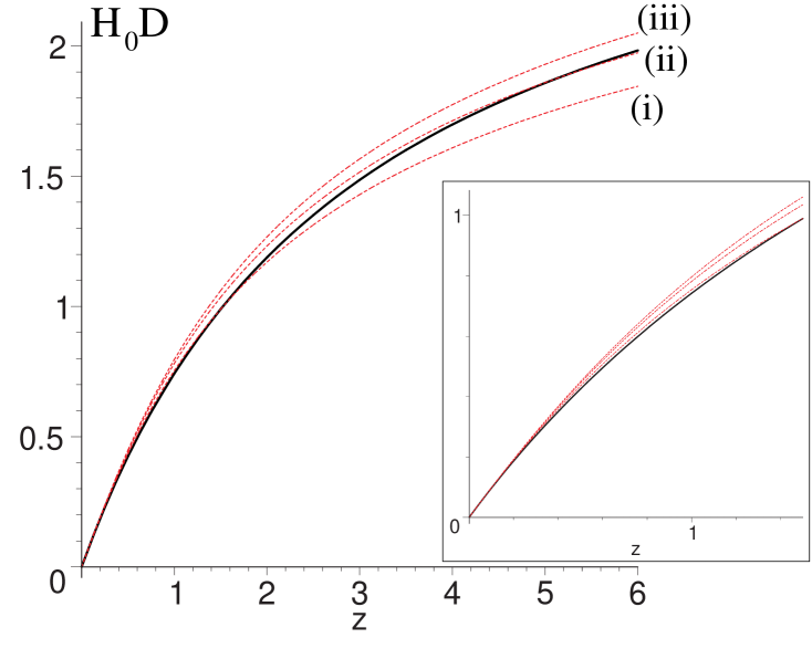
(a)  (b)

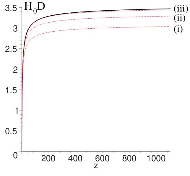
Figure 1: ^∗ The effective comoving distance $H_{\lower 2.0pt\hbox{$\scriptstyle 0$}}D(z)$ is plotted for the best–fit nonlinear bubble model, with $f_{\hbox{\sevenrm v0}}=0.762$, (solid line); and for various spatially flat $\Lambda$CDM models (dashed lines). The parameters for the dashed lines are (i) $\Omega_{\lower 2.0pt\hbox{$\scriptstyle M0$}}=0.34$ (best–fit to SneIa only); (ii) $\Omega_{\lower 2.0pt\hbox{$\scriptstyle M0$}}=0.279$ (joint best–fit to SneIa, BAO and WMAP5); (iii) $\Omega_{\lower 2.0pt\hbox{$\scriptstyle M0$}}=0.249$ best–fit to WMAP5 only. Panel (a) shows the redshift range $z<6$, with an inset for $z<1.5$, the range tested by current SneIa data. Panel (b) shows the range $z<1100$ up to the surface of last scattering, tested by WMAP5.

References

- [2000] Buchert, T. 2000, Gen. Relativ. Grav. 32, 105.
- [2008] Buchert, T. 2008, Gen. Relativ. Grav. 40, 467.
- [2003] Buchert, T. & Carfora, M. 2003, Phys. Rev. Lett. 90, 031101.
- [2007] Célérier, M.N. 2007, New Adv. Phys. 1, 27. [astro-ph/0702416]
- [2002] Hoyle, F. & Vogeley, M.S. 2002, ApJ 566, 641.
- [2004] Hoyle, F. & Vogeley, M.S. 2004, ApJ 607, 751.
- [2006] Ishibashi, A. & Wald, R.M. 2006, Class. Quantum Grav. 23, 235.
- [1] Jha, S., Riess A.G. & Kirshner, R.P. 2007, ApJ 659, 122.
- [2] Komatsu, E. et al. 2009, ApJ Suppl. 180, 330.
- [2008] Leith, B.M., Ng, S.C.C. & Wiltshire, D.L. 2008, ApJ 672, L91.
- [3] Li, N. & Schwarz, D.J. 2008, Phys. Rev. D 78, 083531.
- [2007] Riess, A.G. et al. 2007, ApJ 659, 98.
- [2006] Sandage, A. et al. 2006, ApJ 653, 843.
- [2007] Wiltshire, D.L. 2007a, New J. Phys. 9, 377.
- [2007] Wiltshire, D.L. 2007b, Phys. Rev. Lett. 99, 251101.
- [2008] Wiltshire, D.L. 2008, Phys. Rev. D 78, 084032.
- [2009] Wiltshire, D.L. 2009, Phys. Rev. D 80, 123512.