Abstract

Given a power grid modeled by a network together with equations describing the power flows, power generation and consumption, and the laws of physics, the so-called $N-k$ problem asks whether there exists a set of $k$ or fewer arcs whose removal will cause the system to fail. The case where $k$ is small is of practical interest. We present theoretical and computational results involving a mixed-integer model and a continuous nonlinear model related to this question.

1 Introduction

Recent large-scale power grid failures have highlighted the need for effective computational tools for analyzing vulnerabilities of electrical transmission networks. Blackouts are extremely rare, but their consequences can be severe. Recent blackouts had, as their root cause, an exogenous damaging event (such as a storm) which developed into a system collapse even though the initial quantity of disabled power lines was small.

As a result, a problem that has gathered increasing importance is what might be termed the vulnerability evaluation problem: given a power grid, is there a small set of power lines whose removal will lead to system failure? Here, “smallness” is parametrized by an integer $k$, and indeed experts have called for small values of $k$ (such as $k=3$ or $4$) in the analysis. Additionally, an explicit goal in the formulation of the problem is that the analysis should be agnostic: we are interested in rooting out small, “hidden” vulnerabilities of a complex system which is otherwise quite robust; as much as possible the search for such vulnerabilities should be devoid of assumptions regarding their structure.

This problem is not new, and researchers have used a variety of names for it: network interdiction, network inhibition and so on, although the “N - k problem” terminology is common in the industry. Strictly speaking, one could consider the failure of different types of components (generators, transformers) in addition to lines, however, in this paper “N” will represent the number of lines. We will provide a more complete review of the literature later on; the core central theme is that the $N-k$ problem is intractable, even for small values of $k$ – the pure enumeration approach is simply impractical. In addition to the combinatorial explosion, another significant difficulty is the need to model the laws of physics governing power flows in a sufficiently accurate and yet computationally tractable manner: power flows are much more complex than “flows” in traditional computer science or operations research applications.

A critique that has been leveled against optimization-based approaches to the $N-k$ problem is that they tend to focus on large values of $k$, say $k=8$. In our experience, when $k$ is large the problem tends to become easier (possibly because many solutions exist) but on the other hand the argument can be made that the cardinality of the attack is unrealistically large. At the other end of the spectrum lies the case $k=1$, which can be addressed by enumeration but may not yield useful information. The middle range, $2\leq k\leq 5$, is both relevant and difficult, and is our primary focus.

We present results using two optimization models. The first (Section 2.1) is a new linear mixed-integer programming formulation that explicitly models a “game” between a fictional attacker seeking to disable the network, and a controller who tries to prevent a collapse by selecting which generators to operate and adjusting generator outputs and demand levels. As far as we can tell, the problem we consider here is more general than has been previously studied in the literature; nevertheless our approach yields practicable solution times for larger instances than previously studied.

The second model (Section 3) is given by a new, continuous nonlinear programming formulation whose goal is to capture, in a compact way, the interaction between the underlying physics and the network structure. While both formulations provide substantial savings over the pure enumerational approach, the second formulation appears particularly effective and scalable; enabling us to handle in an optimization framework models an order of magnitude larger than those we have seen in the literature.

1.0.1 Previous work on vulnerability problems

There is a large amount of prior work on optimization methods applied to blackout-related problems. [21] includes a fairly comprehensive survey of recent work.

Typically work has focused on identifying a small set of arcs whose removal (to model complete failure) will result in a network unable to deliver a minimum amount of demand. A problem of this type can be solved using mixed-integer programming techniques techniques, see [3], [22], [4]. We will review this work in more detail below (Section 2.0.2). Generally speaking, the mixed-integer programs to be solved can prove quite challenging.

A different line of research on vulnerability problems focuses on attacks with certain structural properties, see [7], [21]. An example of this approach is used in [21], where as an approximation to the $N-k$ problem with AC power flows, a linear mixed-integer program to solve the following combinatorial problem: remove a minimum number of arcs, such that in the resulting network there is a partition of the nodes into two sets, $N_{1}$ and $N_{2}$, such that

$$D(N_{1})\,+\,G(N_{2})\,+\,cap(N_{1},N_{2})\,\leq\,Q^{min}.$$ (1)

Here $D(N_{1})$ is the total demand in $N_{1}$, $G(N_{2})$ is the total generation capacity in $N_{2}$, $cap(N_{1},N_{2})$ is the total capacity in the (non-removed) arcs between $N_{1}$ and $N_{2}$, and $Q^{min}$ is a minimum amount of demand that needs to be satisfied. The quantity in the left-hand side in the above expression is an upper-bound on the total amount of demand that can be satisfied – the upper-bound can be strict because under power flow laws it may not be attained.

Thus this is an approximate model that could underestimate the effect of an attack (i.e. the algorithm may produce attacks larger than strictly necessary). On the other hand, methods of this type bring to bear powerful mathematical tools, and thus can handle larger problems than algorithms that rely on generic mixed-integer programming techniques. Our method in Section 3 can also be viewed as an example of this approach.

Finally, we mention that the most sophisticated models for the behavior of a grid under stress attempt to capture the multistage nature of blackouts, and are thus more comprehensive than the static models considered above and in this paper. See, for example, [10]-[13], and [6].

1.0.2 Power Flows

Here we provide a brief introduction to the so-called linearized, or DC power flow model. For the purposes of our problem, a grid is represented by a directed network ${\cal N}$, where:

• Each node corresponds to a “generator” (i.e., a supply node), or to a “load” (i.e., a demand node), or to a node that neither generates nor consumes power. We denote by ${\cal G}$ the set of generator nodes.

• If node $i$ corresponds to a generator, then there are values $0\leq P_{i}^{min}\leq P_{i}^{max}$. If the generator is operated, then its output must be in the range $[P_{i}^{min},P_{i}^{max}]$; if the generator is not operated, then its output is zero. In general, we expect $P^{min}_{i}>0$.

• If node $i$ corresponds to a demand, then there is a value $D_{i}^{nom}$ (the “nominal” demand value at node $i$). We will denote the set of demands by ${\cal D}$.

• The arcs of ${\cal N}$ represent power lines. For each arc $(i,j)$, we are given a parameter $x_{ij}>0$ (the resistance) and a parameter $u_{ij}$ (the capacity).

Given a set ${\cal C}$ of operating generators, a power flow is a solution to the system of constraints given next. In this system, for each arc $(i,j)$, we use a variable $f_{ij}$ to represent the (power) flow on $(i,j)$ – possibly $f_{ij}<0$, in which case power is effectively flowing from $j$ to $i$. In addition, for each node $i$ we will have a variable $\theta_{i}$ (the “phase angle” at $i$). Finally, if $i$ is a generator node, then we will have a variable $P_{i}$, while if $i$ represents a demand node, we will have a variable $D_{i}$. Given a node $i$, we represent with $\delta^{+}(i)$ ($\delta^{-}(i)$) the set of arcs oriented out of (respectively, into) $i$.

In the system given below, hereafter denoted by ${P({\cal N},{\cal C})}$, constraints (5), (8) and (9) are typical for network flow models (for background see [1]) and model, respectively: flow balance (i.e., net flow leaving a node equals net supply at that node), generator and demand node bounds. Constraint (6) is a commonly used linearization of more complex equations describing power flow physics; for background see [2]. We will comment on this equation in Section 1.0.4.

$$\sum_{(i,j)\in\delta^{+}(i)}f_{ij}-\sum_{(j,i)\in\delta^{-}(i)}f_{ji}=\left\{\begin{array}[]{lll}~{}~{}P_{i}&{i\in{\cal C}}&\\ -D_{i}&{i\in{\cal D}}&\\ ~{}~{}0&\mbox{otherwise}&\end{array}\right.$$ (5)

$$\theta_{i}-\theta_{j}-x_{ij}f_{ij}=0\ \ \ \forall(i,j)$$ (6)

$$|f_{ij}|\ \ \ \leq\ \ \ u_{ij},\ \ \ \forall(i,j)$$ (7)

$$P_{i}^{min}\leq P_{i}\leq P_{i}^{max}\ \ \ \forall i\in{\cal C}$$ (8)

$$0\leq D_{j}\leq D_{j}^{nom}\ \ \ \forall j\in{\cal D}$$ (9)

One could also impose explicit upper bounds on the quantities $|\theta_{i}-\theta_{j}|$ (over the arcs $(i,j)$). However, note that our model already does so, implicitly: because of constraint (6), imposing an upper bound on $|f_{ij}|$ (i.e., eq. (7)) is equivalent to imposing an upper bound on $|\theta_{i}-\theta_{j}|$.

1.0.3 Basic properties

A useful property satisfied by the linearized model is given by the following result.

Lemma 1.1

Let ${\cal C}$ be given, and suppose ${\cal N}$ is connected. Then for any choice of nonnegative values $P_{i}$ (for $i\in{\cal C}$) and $D_{i}$ (for $i\in{\cal D}$) such that

$$\sum_{i\in{\cal C}}P_{i} = \sum_{i\in{\cal D}}D_{i},$$ (10)

system (5)-(6) has a unique solution in the $f_{ij}$; thus, the solution is also unique in the $\theta_{i}-\theta_{j}$ (over the arcs $(i,j)$).

Proof. Let $N$ denote the node-arc incidence of the network [1], let $b$ be the vector with an entry for each node, where $b_{i}=P_{i}$ for $i\in{\cal C}$, $b_{i}=-D_{i}$ for $i\in{\cal D}$, and $b_{i}=0$ otherwise. Writing $X$ for the diagonal matrix with entries $x_{ij}$, then (5)-(6) can be summarized as

$$Nf = b,$$ (11)

$$N^{T}\theta\,-\,Xf = 0.$$ (12)

Pick an arbitrary node $v$; then system (11)-(12) has a solution iff it has one with $\theta_{v}=0$. As is well-known, $N$ does not have full row rank, but writing $\bar{N}$ for the submatrix of $N$ with the row corresponding to $v$ omitted then the connectivity assumption implies that $\bar{N}$ does have full row rank [1]. In summary, writing $\bar{b}$ for the corresponding subvector of $b$, we have that (11)-(12) has a solution iff

$$\bar{N}f = \bar{b},$$ (13)

$$\bar{N}^{T}\eta\,-\,Xf = 0.$$ (14)

where the vector $\eta$ has an entry for every node other than $v$. Here, (14) implies $f=X^{-1}\bar{N}^{T}\eta$, and so (13) implies that $\eta=(\bar{N}X^{-1}\bar{N}^{T})^{-1}\bar{b}$ (where the matrix is invertible since $\bar{N}$ has full row rank). Consequently, $f=X^{-1}\bar{N}^{T}(\bar{N}X^{-1}\bar{N}^{T})^{-1}\bar{b}$.  

Remark 1.2

We stress that Lemma 1.1 concerns the subsystem of ${P({\cal N},{\cal C})}$ consisting of (5) and (6). In particular, the “capacities” $u_{ij}$ play no role in the determination of solutions.

When the network is not connected Lemma 1.1 can be extended by requiring that (10) hold for each component.

Definition 1.3

Let $(f,\theta,P,D)$ be feasible a solution to $P({\cal N},{\cal C})$. The throughput of $(f,\theta,P,D)$ is defined as

$$\frac{\sum_{i\in{\cal D}}D_{i}}{\sum_{i\in{\cal D}}D^{nom}_{i}}.$$ (15)

The throughput of ${\cal N}$ is the maximum throughput of any feasible solution to $P({\cal N},{\cal C})$.

1.0.4 DC and AC power flows, and other modeling issues

Constraint (6) is reminiscent of Ohm’s equation – in a direct current (DC) network (6) precisely represents Ohm’s equation. In the case of an AC network (the relevant case when dealing with power grids) (6) only approximates a complex system of nonlinear equations (see [2]). The issue of whether to use the more accurate nonlinear formulation, or the approximate DC formulation, is rather thorny. On the one hand, the linearized formulation certainly is an approximation only. On the other hand, a formulation that models AC power flows can prove intractable or may reflect difficulties inherent with the underlying real-life problem (e.g. the formulation may have multiple solutions).

We can provide a very brief summary of how the linearized model arises. First, AC power flow models typically include equations of the form

$$x_{ij}f_{ij} = \sin(\theta_{i}-\theta_{j}),\ \ \ \forall(i,j),$$ (16)

as opposed to (6). Here, the $f$ quantities describe “active” power flows and the $\theta$ describe phase angles. In normal operation of a transmission system, one would expect that $\theta_{i}\approx\theta_{j}$ for any arc $(i,j)$ and thus (16) can be linearized to yield (6). Hence the linearization is only valid if we additionally impose that $|\theta_{i}-\theta_{j}|$ be very small. However, in the literature one sometimes sees this “very small” constraint relaxed, for the reason that we are interested in regimes where the network is not in a normal operative mode. One might still impose some explicit upper bound on $|\theta_{i}-\theta_{j}|$; we have seen publications with and without such a constraint. As explained above, our model already includes such a constraint in implicit form.

In either case, one ends up using a representation of the problem that is arguably not valid. But the key fact is that constraint (16) gives rise to extremely complex models. Studies that require multiple power flow computations tend to rely on the linearized formulation, in the expectation that some useful information will emerge. This will be the approach we take in this paper, though some of our techniques extend directly to AC models and this will remain a topic for future research.

An approach such as ours can therefore be criticized because it relies on an ostensibly approximate model; on the other hand we are able to focus more explicitly on the basic combinatorial complexity that underlies the $N-k$ problem. In contrast, an approach addressing AC model characteristics would have a better representation of the physics, but at the cost of not being able to tackle the combinatorial complexity quite as effectively, for the simple reason that the theory and computational machinery for linear programming are far more mature, effective and scalable than those for nonlinear, nonconvex optimization. In summary, both approaches present limitations and benefits. In this paper, our bias is toward explicitly handling the combinatorial nature of the problem.

A final point that we would like to stress is that whether we use an AC or DC power flow model, the resulting problems have a far more complex structure than (say) traditional single- or multi-commodity flow models because of side-constraints such as (6). Constraints of this type give rise to counter-intuitive behavior reminiscent of Braess’s Paradox [9].

The model we consider in the paper can be further enriched by including many other real-life constraints. For example, when considering the response to a contingency one could insist that demand be curtailed in a (geographically) even-handed pattern, and not in an aggregate fashion, as we do below and has been done in the literature. Or we could impose upper bounds on the number of stand-by power units that are turned on in the event of a contingency (and this itself could have a geographical perspective). Many such realistic features suggest themselves and could give rise to interesting extensions to the problem we consider here.

2 The “N - k” problem

Let ${\cal N}$ be a network with $n$ nodes and $m$ arcs representing a power grid. We denote the set of arcs by $E$ and the set of nodes by $V$. A fictional attacker wants to remove a small number of arcs from ${\cal N}$ so that in the resulting network all feasible flows should have low throughput. At the same time, a controller is operating the network; the controller responds to an attack by appropriately choosing the set ${\cal C}$ of operating generators, their output levels, and the demands $D_{i}$, so as to feasibly obtain high throughput. Note that the controller’s adjustment of demands corresponds to the traditional notion of “load shedding” in the power systems literature.

Thus, the attacker seeks to defeat all possible courses of action by the controller, in other words, we are modeling the problem as a Stackelberg game between the attacker and the controller, where the attacker moves first. To cast this in a precise way we will use the following definition. We let $0\leq T^{min}\leq 1$ be a given value.

Definition 2.1

Given a network ${\cal N}$,

• An attack ${\cal A}$ is a set of arcs removed by the attacker.

• Given an attack ${\cal A}$, the surviving network ${\cal N}-{\cal A}$ is the subnetwork of ${\cal N}$ consisting of the arcs not removed by the attacker.

• A configuration is a set ${\cal C}$ of generators.

• We say that an attack ${\cal A}$ defeats a configuration ${\cal C}$, if either (a) the maximum throughput of any feasible solution to ${P({\cal N}-{\cal A},{\cal C})}$ is strictly less than $T^{min}$, or (b) no feasible solution to ${P({\cal N}-{\cal A},{\cal C})}$ exists. Otherwise we say that ${\cal C}$ defeats ${\cal A}$.

• We say that an attack is successful, if it defeats every configuration.

• The min-cardinality attack problem consists in finding a successful attack ${\cal A}$ with $|{\cal A}|$ minimum.

Our primary focus will be on the min-cardinality attack problem. Before proceeding further we would like to comment on our model, specifically on the parameter $T^{min}$. In a practical use of the model, one would wish to experiment with different values for $T^{min}$ – for the simple reason that an attack ${\cal A}$ which is not successful for a given choice for $T^{min}$ could well be successful for a slightly larger value; e.g. no attack of cardinality $3$ or less exists that reduces demand by $31\%$, and yet there exists an attack of cardinality $3$ that reduces satisfied demand by $30\%$. In other words, the minimum cardinality of a successful attack could vary substantially as a function of $T^{min}$.

Given this fact, it might appear that a better approach to the power grid vulnerability problem would be to leave out the parameter $T^{min}$ entirely, and instead redefine the problem to that of finding a set of $k$ or fewer arcs to remove, so that the resulting network has minimum throughput (here, $k$ is given). We will refer to this as the budget-k min-throughput problem. However, there are reasons why this latter problem is less attractive than the min-cardinality problem.

• The min-cardinality and min-throughput problems are duals of each other. A modeler considering the min-throughput problem would want to run that model multiple times, because given $k$, the value of the budget-$k$ min-throughput problem could be much smaller than the value of the budget-$(k+1)$ min-throughput problem. For example, it could be the case that using a budget of $k=2$, the attacker can reduce throughput by no more than $5\%$; but nevertheless with a budget of $k=3$, throughput can be reduced by e.g. $50\%$. In other words, even if a network is “resilient” against attacks of size $\leq 2$, it might nevertheless prove very vulnerable to attacks of size $3$. For this reason, and given that the models of grids, power flows, etc., are rather approximate, a practitioner would want to test various values of $k$ – this issue is obviously related to what percentage of demand loss would be considered tolerable, in other words, the parameter $T^{min}$.

• From an operational perspective it should be straightforward to identify reasonable values for the quantity $T^{min}$; whereas the value $k$ is more obscure and bound to models of how much power the adversary can wield.

• Because of a subtlety that arises from having positive quantities $P^{min}_{i}$, explained next, it turns out that the min-throughput problem is significantly more complex and is difficult to even formulate in a compact manner.

We will now expand on (c). One would expect that when a configuration ${\cal C}$ is defeated by an attack ${\cal A}$, it is because only small throughput solutions are feasible in ${\cal N}-{\cal A}$. However, because the lower bounds $P_{i}^{min}$ are in general strictly positive, it may also be the case that no feasible solution to ${P({\cal N}-{\cal A},{\cal C})}$ exists.

Example 2.2

Consider the following example on a network ${\cal N}$ with three nodes (see Figure 1), where

1. Nodes $1$ and $2$ represent generators; $P^{min}_{1}=2$, $P^{max}_{1}=4$, $P^{min}_{2}=0$, and $P^{max}_{2}=4$,

2. Node $3$ is a demand node with $D^{nom}_{3}=6$. Furthermore, $T^{min}=1/2$.

3. There are three arcs; arc $(1,2)$ with $x_{12}=1$ and $u_{12}=1$, arc $(2,3)$ with $x_{23}=1$ and $u_{23}=5$, and arc $(1,3)$ with $x_{13}=1$ and $u_{13}=3$.

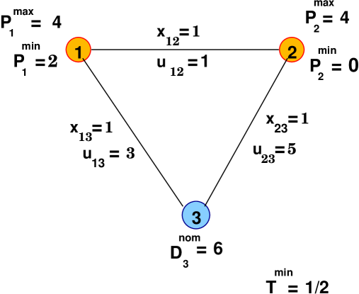
Figure 1: A simple example where the controller must turn off a generator.

When the network is not attacked, the following solution is feasible: $P_{1}=P_{2}=3$, $D_{3}=6$, $f_{12}=0$, $f_{13}=f_{23}=3$, $\theta_{1}=\theta_{2}=0$, $\theta_{3}=-3$. This solution has throughput $100\%$. On the other hand, consider the attack ${\cal A}$ consisting of the single arc $(1,3)$. Since $P^{min}_{1}>u_{12}$, ${P({\cal N}-{\cal A},{\cal C})}$ has no feasible solution, and ${\cal A}$ defeats ${\cal C}$, for ${\cal C}=\{1,2\}$ or ${\cal C}=\{1\}$, in spite of the fact that that total generator capacity is enough to meet at least $2/3>T^{min}$ of the demand. Thus, ${\cal A}$ is successful if and only if it also defeats the configuration where we only operate generator $2$, which it does not since in that configuration we can feasibly send up to four units of flow on $(2,3)$.

As the example highlights, it is important to understand how an attack ${\cal A}$ can defeat a particular configuration ${\cal C}$. It turns out that there are three different ways for this to happen.

• Consider a partition of the nodes of ${\cal N}$ into two classes, $N^{1}$ and $N^{2}$. Write

  $$D^{k} = \sum_{i\in{\cal D}\cap N^{k}}D^{nom}_{i},\,\,\,\,k=1,2,\,\,\,\,\,\,\mbox{and}$$ (17)

  $$P^{k} = \sum_{i\in{\cal C}\cap N^{k}}P^{max}_{i},\,\,\,\,k=1,2,$$ (18)

  e.g. the total (nominal) demand in $N_{1}$ and $N_{2}$, and the maximum power generation in $N_{1}$ and $N_{2}$, respectively. The following condition, should it hold, would guarantee that ${\cal A}$ defeats ${\cal C}$:

  $$T^{min}\sum_{j\in{\cal D}}D^{nom}_{j}-\min\{D^{1},P^{1}\}-\min\{D^{2},P^{2}\} > \sum_{(i,j)\notin{\cal A}\,:\,i\in N^{1},\,j\in N^{2}}u_{ij}\,+\,$$ (19)

  $$\,\,\,\,\,\sum_{(i,j)\notin{\cal A}\,:\,i\in N^{2},\,j\in N^{j}}u_{ij}.$$

  To understand this condition, note that for $k=1,2$, $\min\{D^{k},P^{k}\}$ is the maximum demand within $N^{k}$ that could possibly be met using power flows that do not leave $N^{k}$. Consequently the left-hand side of (19) is a lower bound on the amount of flow that must travel between $N^{1}$ and $N^{2}$, whereas the right-hand side of (19) is the total capacity of arcs between $N^{1}$ and $N^{2}$ under attack ${\cal A}$. In other words, condition (19) amounts to a mismatch between demand and supply. A special case of (19) is that where in ${\cal N}-{\cal A}$ there are no arcs between $N^{1}$ and $N^{2}$, i.e. the right-hand side of (19) is zero. Condition (20) is similar, but not identical, to (1).

• Consider a partition of the nodes of ${\cal N}$ into two classes, $N^{1}$ and $N^{2}$. Then attack ${\cal A}$ defeats ${\cal C}$ if

  $$\sum_{i\in{\cal D}\cap\in N^{1}}D^{nom}_{i}\ +\ \sum_{(i,j)\notin{\cal A}\,:\,i\in N^{1},\,j\in N^{2}}u_{ij} < \sum_{i\in{\cal C}\cap N^{1}}P^{min}_{i},$$ (20)

  i.e., the minimum power output within $N^{1}$ exceeds the maximum demand within $N^{1}$ plus the sum of arc capacities leaving $N^{1}$. Note that (ii) may apply even if (i) does not.

• Even if (i) and (ii) do not hold, it may still be the case that the system (5)-(9) does not admit a feasible solution. To put it differently, suppose that for every choice of demand values $0\leq D_{i}\leq D^{nom}_{i}$ (for $i\in{\cal D}$) and supply values $P^{min}_{i}\leq P_{i}\leq P^{max}_{i}$ (for $i\in{\cal C}$) such that $\sum_{i\in{\cal C}}P_{i}\,=\,\sum_{i\in{\cal D}}D_{i}$ the unique solution to system (5)-(6) in network ${\cal N}-{\cal A}$ (as per Lemma 1.1) does not satisfy the “capacity” inequalities $|f_{ij}|\leq u_{ij}$ for all arcs $(i,j)\in{\cal N}-{\cal A}$. Then ${\cal A}$ defeats ${\cal C}$. This is the most subtle case of all – it involves the interplay of constraints (6) and (5) in the power flow model.

Note that in particular in case (ii), the defeat condition is unrelated to throughput. Nevertheless, should case (ii) arise, it is clear that the attack has succeeded (against configuration ${\cal C}$) – this makes the min-throughput problem difficult to model; our formulation for the min-cardinality problem, given in Section 2.1, does capture the three defeat criteria above.

From a practical perspective, it is important to handle models where the values $P^{min}_{i}$ are positive. It is also important to model standby generators that are turned on when needed, and to model the turning off of generators that are unable to dispose of their minimum power output, post-attack. All these features arise in practice. Example 2.2 above shows that models where generators cannot be turned off can exhibit unreasonable behavior. Of course, the ability to select the operating generators comes at a cost, in that in order to certify that an attack is successful we need to evaluate, at least implicitly, a possibly exponential number of control possibilities.

As far as we can tell, most (or all) prior work in the literature does require that the controller must always use the configuration $\bar{\cal G}$ consisting of all generators. As the example shows, however, if the quantities $P^{min}_{i}$ are positive there may be attacks ${\cal A}$ such that ${P({\cal N}-{\cal A},\bar{\cal G})}$ is infeasible. Because of this fact, algorithms that rely on direct application of Benders’ decomposition or bilevel programming are problematic, and invalid formulations can be found in the literature.

Our approach works with general $P^{min}\geq 0$ quantities; thus, it also applies to the case where we always have $P^{min}_{i}=0$. In this case our formulation is simple enough that a commercial integer program solver can directly handle instances larger than previously reported in the literature.

2.0.1 Non-monotonicity in optimal attacks

Consider the example in Figure 2, where we assume $T^{min}=0.3$. Notice that there are two parallel copies of arcs $(2,4)$ and $(3,5)$, each with capacity $10$ and impedance $1$. It is easy to see that the network with no attack is feasible: we operate generator $1$ and not operate generators $2$ and $3$, and send $3$ units of flow along the paths $1-6-2-4$ and $1-6-3-5$ (the flow on e.g. the two parallel $(2,4)$ arcs is evenly split).

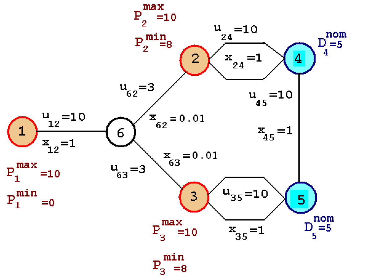
Figure 2: An example where there is a successful attack with $k=1$ but none with $k=2$.

On the other hand, consider the attack consisting of arc $(1,6)$ – we will show this attack is successful. To see this, note that under this attack, the controller cannot operate both generators $2$ and $3$, since their combined minimum output exceeds the total demand. Thus, without loss of generality suppose that only generator $3$ is operated, and assume by contradiction that a feasible solution exists – then this solution must route at most $3$ units of flow along $3-6-2-4$, and (since $P^{min}_{3}=8$) at least $5$ units of flow on $(3,5)$ (both copies altogether). In such a case, the phase angle drop from $3$ to $5$ is at least $2.5$, whereas the drop from $3$ to $4$ is at most $1.56$. In other words, $\theta_{4}-\theta_{5}\geq 0.94$, and so we will have $f_{45}\geq 0.94$ – thus, the net inflow at node $5$ is at least $5.94$. Hence the attack is indeed successful.

However, there is no successful attack consisting of arc $(1,6)$ and another arc. To see this, note that if one of $(2,6)$, $(3,6)$ or $(4,5)$ are also removed then the controller can just operate one of the two generators $2$, $3$ and meet eight units of demand. Suppose that (say) one of the two copies of $(3,5)$ is removed (again, in addition to $(1,6)$). Then the controller operates generator $2$, sending $2.5$ units of flow on each of the two parallel $(2,4)$ arcs; thus $\theta_{2}-\theta_{4}=2.5$. The controller also routes $3$ units of flow along $2-6-3-5$, and therefore $\theta_{2}-\theta_{5}=3.06$. Consequently $\theta_{4}-\theta_{5}=.56$, and $f_{45}=.56$, resulting in a feasible flow which satisfies $4.44$ units of demand at $4$ and $3.56$ units of demand at $5$.

In fact, it can be shown that no successful attack of cardinality $2$ exists – hence we observe non-monotonicity.

By elaborating on the above, one can create examples with arbitrary patterns in the cardinality of successful attacks. One can also generate examples that exhibit non-monotone behavior in response to controller actions. In both cases, the non-monotonicity can be viewed as a manifestation of the so-called “Braess’s Paradox” [9]. In the above example we can observe combinatorial subtleties that arise from the ability of the controller to choose which generators to operate, and from the lower bounds on output in operating generators. Nevertheless, it is clear that the critical core reason for the complexity is the interaction between phase angles and flows, i.e. between “Ohm’s law” (6) and flow conservation (5) – the combinatorial attributes of the problem exercise this interaction.

2.0.2 Brief review of previous work on related problems

The min-cardinality problem, as defined above, can be viewed as a bilevel program where both the master problem and the subproblem are mixed-integer programs – the master problem corresponds to the attacker (who chooses the arcs to remove) and the subproblem to the controller (who chooses the generators to operate). In general, such problems are extremely challenging. A recent general-purpose algorithm for such integer programs is given in [15].

Alternatively, each configuration of generators can be viewed as a “scenario”. In this sense our problem resembles a stochastic program, although without a probability distribution. Recent work [18] considers a single commodity max-flow problem under attack by an interdictor with a limited attack budget; where an attacked arc is removed probabilistically, leading to a stochastic program (to minimize the expected max flow). A deterministic, multi-commodity version of the same problem is given in [19].

Previous work on the power grid vulnerability models proper has focused on cases where either the generator lower bounds $P^{min}_{i}$ are all zero, or all generators must be operated (the single configuration case). Algorithms for these problems have either relied on heuristics, or on mixed-integer programming techniques, usually a direct use of Benders’ decomposition or bilevel programming. [3] considers a version of the min-throughput problem with $P^{min}_{i}=0$ for all generators $i$, and presents an algorithm using Benders’ decomposition (also see references therein). They analyze the so-called IEEE One-Area and IEEE Two-Area test cases, with, respectively, 24 nodes and 38 arcs, and 48 nodes and 79 arcs. Also see [22].

[4] studies the IEEE One-Area test case, and allows $P^{min}_{i}>0$, but does not allow generators to be turned off; the authors present a bilevel programming formulation which unfortunately is incorrect, due to reasons outlined above.

2.1 A mixed-integer programming algorithm for the min-cardinality problem

In this section we will describe an iterative algorithm for the min-cardinality attack problem. The algorithm iterates in Benders-like fashion, solving at each iteration two mixed-integer programs. Before describing the algorithm we need to introduce some notation and concepts.

Let ${\cal A}$ be a given attack. Suppose the controller attempts to defeat the attacker by choosing a certain configuration ${\cal C}$ of generators. Denote by $z^{\cal A}$ the indicator vector for ${\cal A}$, i.e. $z^{\cal A}_{ij}=1$ iff $(i,j)\in{\cal A}$. The controller needs to operate the network so as to satisfy the required amount of demand without exceeding any arc capacity. The last requirement can be cast as an optimization goal: minimize the maximum arc overload subject to satisfying the desired level of demand. Should this min-max overload be strictly greater than 1, the controller is defeated. In summary, the controller needs to solve the following linear program (where the variable “t” indicates the min-max overload):

$$\mbox{{\boldmath${K_{{\cal C}}({\cal A}):}$}}\hskip 43.36243ptt_{{\cal C}}(z^{\cal A}) \doteq\ \mbox{ \ min}\ t$$ (32)

Subject to:

$$\sum_{(i,j)\in\delta^{+}(i)}f_{ij}-\sum_{(j,i)\in\delta^{-}(i)}f_{ji}=\left\{\begin{array}[]{lll}~{}~{}P_{i}&{i\in{\cal G}}&\\ -D_{i}&{i\in{\cal D}}&\\ ~{}~{}~{}0&\mbox{otherwise}&\end{array}\right.$$

$$\theta_{i}-\theta_{j}-x_{ij}f_{ij}=0\ \ \ \forall\ (i,j)\notin{\cal A}$$

$$u_{ij}~{}t\ -\ |f_{ij}|\ \ \ \geq\ \ \ 0,\ \ \ \forall\ (i,j)\notin{\cal A}$$

$$f_{ij}\ \ =\ \ \ 0,\ \ \forall(i,j)\in{\cal A}$$

$$P_{i}^{min}\ \leq P_{i}\ \leq P_{i}^{max}\ \ \ \forall i\in{\cal C}$$

$$P_{i}\ \ =\ \ 0,\ \ \ \forall i\in{\cal G}\ -\ {\cal C}$$

$$\sum_{j\in{\cal D}}D_{j}~{}\geq~{}T^{min}\left(\sum_{j\in{\cal D}}D^{nom}_{j}\right),$$

$$0\leq~{}D_{j}~{}\leq D_{j}^{nom}\ \ \ \forall j\in{\cal D}$$

Remark 2.3

Using the convention that the value of an infeasible linear program is infinite, ${\cal A}$ defeats ${\cal C}$ if and only if $t_{{\cal C}}(z^{\cal A})>1$.

Thus, an attack ${\cal A}$ is not successful if and only if we can find ${\cal C}\subseteq{\cal G}$ with $t_{{\cal C}}(z^{\cal A})\leq 1$; we test for this condition by solving the problem:

$$\min_{{\cal C}\subseteq{\cal G}}~{}t_{{\cal C}}(z^{\cal A}).$$

This is done by replacing, in the above formulation, equations (32), (32) with

$$P_{i}^{min}y_{i}\ \leq P_{i}\ \leq P_{i}^{max}y_{i},\ \ \ \forall i\in{\cal G},$$ (33)

$$y_{i}\ \ =0\ \ \mbox{or}\ \ 1,\ \ \ \forall i\in{\cal G}.$$ (34)

Here, $y_{i}=1$ if the controller operates generator $i$.

The min-cardinality attack problem can now be written as follows:

$$\mbox{ \ min}\ \sum_{(i,j)}z_{ij}$$ (35)

$$t_{{\cal C}}(z)\,>\,1,\,\,\,\,\,\,\forall\,\,{\cal C}\subseteq{\cal G},$$ (36)

$$z_{ij}\,=\,0\,\,\mbox{or}\,\,1,\,\,\,\forall\,\,(i,j).$$ (37)

This formulation, of course, is impractical, because we do not have a compact way of representing any of the constraints (36), and there are an exponential number of them.

Putting these issues aside, we can outline an algorithm for the min-cardinality attack problem. Our algorithm will be iterative, and will maintain a “master attacker” mixed-integer program which will be a relaxation of (35)-(37) – i.e. it will have objective (35) but weaker constraints than (36). Initially, the master attacker MIP will include no variables other than the $z$ variables, and no constraints other than (37). The algorithm proceeds as follows.

Basic algorithm for min-cardinality attack problem
Iterate:

    1. Attacker: Solve master attacker MIP and let $z^{*}$ be its solution. 2. Controller: Search for a set ${\cal C}$ of generators such that $t_{{\cal C}}(z^{*})\,\leq\,1$. (2.a) If no such set ${\cal C}$ exists, EXIT: $\sum_{ij}z^{*}_{ij}$ is the minimum cardinality of a successful attack. (2.b) Otherwise, suppose such a set ${\cal C}$ is found. Add to the master attacker MIP a system of valid inequalities that cuts off $z^{*}$. Go to 1.

As discussed above, the search in Step 2 can be implemented by solving a mixed integer program. Since in 2.b we add valid inequalities to the master, then inductively we always have a relaxation of (35)-(37) and thus the value of the master at any execution of step 1, i.e. the value $\sum_{ij}z^{*}_{ij}$, is a lower bound on the cardinality of any successful attack. Thus the exit condition in step 2.a is correct, since it proves that the attack implied by $z^{*}$ is successful.

The implementation of Case 2.b, on the other hand, requires some care. Assuming we are in case 2.b, we have that $t_{{\cal C}}(z^{*})\leq 1$, and certainly the linear program ${K_{{\cal C}}({\cal A})}$ is feasible. The optimal dual solution would therefore (apparently) furnish a Benders cut that cuts off $z^{*}$. However this would be incorrect since the structure of constraints (32)-(32) depends on $z^{*}$ itself.

Instead, we need to proceed as in two-stage stochastic programming with recourse, where the $z$ variables play the role as “first-stage” variables and also appear in the second-stage problem (the subproblem); solutions to the dual of the second-stage problem can then be used to generate cuts to add to the master problem. Toward this goal, we proceed as follows, given ${\cal C}$ and $z^{*}$:

• Write the dual of $K_{{\cal C}}(\emptyset)$.

• As is standard in interdiction-type problems (see [19], [18], [15], [3]), the dual is then “combinatorialized” by adding the $z$ variables and additional constraints. For example, if $\beta_{ij}$ indicates the dual of constraint (32), then we add, to the dual of $K_{{\cal C}}(\emptyset)$, inequalities of the form

  $$\beta_{ij}-M^{1}_{ij}z_{ij}\leq M^{1}_{ij},\,\,\,-\beta_{ij}-M^{1}_{ij}z_{ij}\leq M^{1}_{ij},$$

  for an appropriate constant $M^{1}_{ij}>0$. We proceed similarly with constraint (32), obtaining the “combinatorial dual”. This combinatorial dual is the functional equivalent of the second-stage problem in stochastic programming.

• Fix the $z_{ij}$ variables in the combinatorial dual to $z^{*}$; this yields a problem that is equivalent to $K_{{\cal C}}(z^{*})$ and (using $v$ to represent the variables in aggregate form) has the general structure

  $$t_{{\cal C}}(z^{*})\,=\, \max\,\,\,c^{T}v$$ (38)

  $$Pv\,\leq\,b\,+\,Qz^{*}.$$

  Here $P$ and $Q$ are matrices, and $b$ is a vector, of appropriate dimensions; and we have a maximization problem since the $K_{{\cal C}}()$ are minimization problems. We obtain a cut of the form

  $$\bar{\alpha}^{T}(b+Qz)\geq 1+\epsilon$$

  where $\epsilon>0$ is a small constant and $\bar{\alpha}$ is the vector of optimal dual variables to (38). Since by assumption $t_{{\cal C}}(z^{*})\leq 1$ this inequality cuts off $z^{*}$.

Note the use of the tolerance $\epsilon$. The use of this parameter gives more power to the controller, i.e. “borderline” attacks are not considered successful. In a strict sense, therefore, we are not solving the optimization problem to exact precision; nevertheless in practice we expect our relaxation to have negligible impact so long as $\epsilon$ is small. A deeper issue here is how to interpret truly borderline attacks that are successful according to our strict model (and which our use of $\epsilon$ disallows); we expect that in practice such attacks would be ambiguous and that the approximations incurred in modeling power flows, estimating demands levels, handling fluctuating demand levels, and so on, not to mention the numerical sensitivity of the integer and linear solvers being used, would have a far more significant impact on precision.

2.1.1 Discussion of the initial formulation

In order to make the outline provided in B.1-B.3 into a formal algorithm, we need to specify the constants $M^{1}_{ij}$. As is well-known, the folklore of integer programming dictates that the $M^{1}_{ij}$ should be chosen small to improve the tightness of the linear programming relaxation of the master problem, that is to say, how close an approximation to the integer program is provided by the LP relaxation.

While this is certainly true, we have found that, additionally, popular optimization packages show significant numerical instability when solving power flow linear programs. In fact, in our experience it is primarily this behavior that mandates that the $M^{1}_{ij}$ should be kept as small as possible. In particular we do not want the $M^{1}_{ij}$ to grow with network since this would lead to an nonscalable approach.

It turns out that our formulation $K_{{\cal C}}({\cal A})$ is not ideal toward this goal. A particularly thorny issue is that the attack ${\cal A}$ may disconnect the network, and proving “reasonable” upper bounds on the dual variables to (for example) constraint (32), when the network is disconnected, does not seem possible. In the next section we describe a different formulation for the min-cardinality attack problem which is much better in this regard. Our eventual algorithm will apply steps B.1 - B.3 to this improved formulation, while the rest of our basic algorithmic methodology as described above will remain unchanged.

2.2 A better mixed-integer programming formulation

As before, let ${\cal A}$ be an attack and ${\cal C}$ a (given) configuration of generators. Let $y^{{\cal C}}\in R^{{\cal G}}$ be the indicator vector for ${\cal C}$, i.e. $y^{{\cal C}}_{i}=1$ if $i\in{\cal C}$ and $y^{{\cal C}}_{i}=0$ otherwise. The linear programming formulation presented below is similar to (32)-(32) except that constraint (46) is used instead of (32), and we use the indicator variables $y^{{\cal C}}$ in equation (47) instead of equation (32). Other differences are explained after the formulation; to the left of each constraint we have indicated corresponding dual variables.

$$\mbox{{\boldmath${K^{*}_{{\cal C}}({\cal A}):}$}}\hskip 43.36243ptt^{*}_{{\cal C}}(z^{\cal A}) \doteq\ \mbox{ \ min}\ t$$ (39)

Subject to:

$${(\alpha^{{\cal C}}_{i})} \sum_{(i,j)\in\delta^{+}(i)}f_{ij}-\sum_{(j,i)\in\delta^{-}(i)}f_{ji}=\left\{\begin{array}[]{lll}~{}~{}P_{i}&{i\in{\cal G}}&\\ -D_{i}&{i\in{\cal D}}&\\ ~{}~{}~{}0&\mbox{otherwise}&\end{array}\right.$$ (43)

$${(\beta^{{\cal C}}_{ij})} \theta_{i}-\theta_{j}-x_{ij}f_{ij}=0\ \ \ \forall\ (i,j)\notin{\cal A}$$ (44)

$${(p^{{\cal C}}_{ij},q^{{\cal C}}_{ij})} u_{ij}~{}t\ -\ |f_{ij}|\ \ \ \geq\ \ \ 0,\ \ \ \forall\ (i,j)\notin{\cal A}$$ (45)

$${(\omega_{ij}^{{\cal C}+},\omega_{ij}^{{\cal C}-})} t\ -\ |f_{ij}|\ \ \ \geq\ \ \ 1,\ \ \ \forall\ (i,j)\in{\cal A}$$ (46)

$${(\gamma^{{\cal C}+}_{i},\gamma^{{\cal C}+}_{i})} P_{i}^{min}y^{{\cal C}}_{i}\ \leq P_{i}\ \leq P_{i}^{max}y^{{\cal C}}_{i}\ \ \ \forall i\in{\cal G}$$ (47)

$${(\mu^{{\cal C}})} \sum_{j\in{\cal D}}D_{j}~{}\geq~{}T^{min}\left(\sum_{j\in{\cal D}}D^{nom}_{j}\right),$$ (48)

$${(\Delta^{{\cal C}}_{j})} D_{j}~{}\leq D_{j}^{nom}\ \ \ \forall j\in{\cal D}$$ (50)

$$P\geq 0,\ \ \ D\geq 0.$$

Note that (45) can be represented as two linear inequalities, and the same applies to (46).

Also, we do not force $f_{ij}=0$ for $(i,j)\in{\cal A}$. Thus, the controller has significantly more power than in $K_{{\cal C}}({\cal A})$. However, because of constraint (46), we have $t^{*}_{{\cal C}}(z^{\cal A})>1$ as soon as any of the arcs in ${\cal A}$ actually carries flow. We can summarize these remarks as follows:

Remark 2.4

${\cal A}$ defeats ${\cal C}$ if and only if $t^{*}_{{\cal C}}(z^{\cal A})>1$.

The above formulation depends on ${\cal C}$ only through constraint (47). Using appropriate matrices $\bar{A}_{f},\bar{A}_{\theta},\bar{A}_{P},\bar{A}_{D},\bar{A}_{t}$, and vector $\hat{b}$, (39)-(50) can be abbreviated as

$$\mbox{{\boldmath${K^{*}_{{\cal C}}({\cal A}):}$}}\hskip 43.36243ptt^{*}_{{\cal C}}(z^{\cal A}) \doteq\ \mbox{ \ min}\ t$$

Subject to:

$$\bar{A}_{f}f\,+\bar{A}_{\theta}\theta\,+\bar{A}_{P}P\,+\bar{A}_{D}D\,+\bar{A}_{t}t\,\,\geq\,\,\bar{b}$$

$$P_{i}^{min}y^{{\cal C}}_{i}\ \leq P_{i}\ \leq P_{i}^{max}y^{{\cal C}}_{i},\ \ \ \forall i\in{\cal G}$$

Allowing the $y$ quantities to become $0/1$ variables, we obtain the problem

$$\hskip 43.36243ptt^{*}(z^{\cal A}) \doteq\ \mbox{ \ min}\ t$$ (51)

Subject to: (54)

$$\bar{A}_{f}f\,+\bar{A}_{\theta}\theta\,+\bar{A}_{P}P\,+\bar{A}_{D}D\,+\bar{A}_{t}t\,\,\geq\,\,\bar{b}$$

$$P_{i}^{min}y_{i}\ \leq P_{i}\ \leq P_{i}^{max}y_{i},\ \ \ \forall i\in{\cal G}$$

$$y_{i}\,\,=\,\,0\,\,\mbox{or}\,\,1,\ \ \ \forall i\in{\cal G}.$$

This is the controller’s problem: we have that $t^{*}(z^{\cal A})\leq 1$ if and only if there exists some configuration of the generators that defeats ${\cal A}$.

However, for the purposes of this section, we will assume ${\cal C}$ is given and that the $y^{{\cal C}}$ are constants. We can now write the dual of $K^{*}_{{\cal C}}({\cal A})$, suppressing the index ${\cal C}$ from the variables, for clarity.

$$\mathbf{A_{{\cal C}}({\cal A})}: \sum_{i\in cG}y^{{\cal C}}_{i}P_{i}^{min}\gamma_{i}^{-}-\sum_{i\in{\cal G}}y^{{\cal C}}_{i}P_{i}^{max}\gamma_{i}^{+}-\sum_{j\in{\cal D}}D_{j}^{nom}\Delta_{j}+\sum_{j\in{\cal D}}D^{nom}_{j}\,\mu_{j}+\sum_{(i,j)\in E}(\omega_{ij}^{+}+\omega_{ij}^{-})$$ max

Subject to: (55)

$$(f_{ij}) \alpha_{i}-\alpha_{j}-x_{ij}\beta_{ij}-p_{ij}+q_{ij}+\omega_{ij}^{+}-\omega_{ij}^{-}\,\,=\,\,0\ \ \forall(i,j)\in E$$

$$(\theta_{i}) \sum_{(i,j)\in\delta^{+}(i)}\beta_{ij}-\sum_{(j,i)\in\delta^{-}(i)}\beta_{ji}\,\,=\,\,0\ \ \forall i\in V$$ (56)

$$(t) \sum_{(i,j)\in E}u_{ij}(p_{ij}+q_{ij})+\sum_{(i,j)\in E}(\omega_{ij}^{+}+\omega_{ij}^{-})\,\,\,\leq\,\,\,1$$ (57)

$$(P_{i}) -\alpha_{i}-\gamma_{i}^{-}+\gamma_{i}^{+}\,\,=\,\,0\ \ \forall i\in{\cal G}$$ (58)

$$(D_{j}) \alpha_{j}+\mu-\Delta_{j}\,\,\leq 0\,\,\ \ \forall j\in{\cal D}$$ (59)

$$(\xi^{+}_{ij},\xi^{-}_{ij}) x_{ij}^{1/2}|\beta_{ij}|\,\,\leq\,\,\mathbf{M}(1-z^{{\cal A}}_{ij})\ \ \forall(i,j)\in E$$ (60)

$$(\varrho_{ij}) p_{ij}+q_{ij}\,\,\leq\,\,\frac{1}{u_{ij}}(1-z^{{\cal A}}_{ij})\ \ \forall(i,j)\in E$$ (61)

$$(\eta_{ij}) \omega_{ij}^{+}+\omega_{ij}^{-}\,\,\leq\,\,z^{{\cal A}}_{ij}\ \ \forall(i,j)\in E$$

$$\omega_{ij}^{+}\geq 0,\ \ \omega_{ij}^{-}\geq 0,\ \ p_{ij}\,\,\geq\,\,0,\ \ q_{ij}\geq 0\ \ \forall(i,j)\in E$$

$$\gamma^{+}_{i},\gamma^{-}_{i}\,\,\geq\,\,0\ \ \forall i\in{\cal G}$$

$$\Delta_{j}\geq 0\ \ \forall j\in{\cal D}$$

$$\mu\geq 0$$

$$\delta_{ij},\ \beta_{ij}\ \mbox{free}\ \ \forall(i,j)\in E$$

$$\alpha_{i}\ \mbox{free}\ \ \forall i\in V.$$

As before, for each constraint we indicate the corresponding dual variable. In (60), $\mathbf{M}$ is an appropriately chosen constant (we will provide a precise value for it below). Note that we are scaling $\beta_{ij}$ by $x_{ij}^{1/2}$ – this is allowable since $x_{ij}^{1/2}>0$; the reason for this scaling will become clear below.

Denoting

$$\psi^{{\cal C}}\ :=\ (\alpha^{{\cal C}},\beta^{{\cal C}},p^{{\cal C}},q^{{\cal C}},\omega^{{\cal C}+},\omega^{{\cal C}-},\gamma^{{\cal C}-},\gamma^{{\cal C}+},\mu^{{\cal C}},\Delta^{{\cal C}})$$

we have that $A_{{\cal C}}({\cal A})$ can be rewritten as:

$$\max\left\{\,w_{{\cal C}}^{T}\,\psi^{{\cal C}}\,:\,A\psi^{{\cal C}}\,\leq\,b\,+\,B\left(1-z^{{\cal A}}\right)\,\right\}$$ (63)

where $A$, $B$, $w_{{\cal C}}$ and $b$ are appropriate matrices and vectors. Consequently, we can now rewrite the min-cardinality attack problem:

$$\mbox{ \ min}\,\,\sum_{(i,j)}z_{ij}$$ (64)

$$\mbox{Subject to:}\ \ \ \ \ \ \ \ \ \ \ \ \ \ \ \ \ t^{{\cal C}} \geq 1+\epsilon,\,\,\,\,\,\,\forall\,\,{\cal C}\subseteq{\cal G}$$ (65)

$$w_{{\cal C}}^{T}\,\psi^{{\cal C}}\,-\,t^{{\cal C}} \geq 0,\,\,\,\,\,\,\forall\,\,{\cal C}\subseteq{\cal G},$$ (66)

$$A\psi^{{\cal C}}\,+\,Bz \leq b\,+\,B\,\,\,\,\,\,\forall\,\,{\cal C}\subseteq{\cal G},$$ (67)

$$z_{ij} = 0\,\,\mbox{or}\,\,1,\,\,\,\forall\,\,(i,j).$$ (68)

This formulation, of course, is exponentially large. An alternative is to use Benders cuts – having solved the linear program $A_{{\cal C}}({\cal A})$, let $(\bar{f},\bar{\theta},\bar{t},\bar{P},\bar{D},\bar{\xi}^{+},\bar{\xi}^{-},\bar{\varrho},\bar{\eta})$ be optimal dual variables. Then the resulting Benders cut is

$$t^{{\cal C}}+\sum_{(i,j)\in E}((\bar{\xi}^{+}_{ij}+\bar{\xi}^{-}_{ij})\mathbf{M}(1-z_{ij}))+\sum_{(i,j)\in E}(\frac{1}{u_{ij}}\bar{\varrho}_{ij}(1-z_{ij}))+\sum_{(i,j)\in E}\bar{\eta}_{ij}z_{ij}\geq 1+\epsilon,$$ (69)

We can now update our algorithmic template for the min-cardinality problem.

Updated algorithm for min-cardinality attack problem
Iterate:

    1. Attacker: Solve master attacker MIP, obtaining attack ${\cal A}$. 2. Controller: Solve the controller’s problem (51)-(54) to search for a set ${\cal C}$ of generators such that $t^{*}_{{\cal C}}(z^{\cal A})\,\leq\,1$. (2.a) If no such set ${\cal C}$ exists, EXIT: ${\cal A}$ is a minimum cardinality successful attack. (2.b) Otherwise, suppose such a set ${\cal C}$ is found. Then (2.b.1) Add to the master the Benders’ cut (69), and, optionally (2.b.2) Add to the master the entire system (65)-(67), Go to 1.

Clearly, option (2.b.2) can only be exercised sparingly. Below we will discuss how we choose, in our implementation, between (2.b.1) and (2.b.2). We will also describe how to (significantly) strengthen the straightforward Benders cut (69). One point to note is that the cuts (or systems) arising from different configurations ${\cal C}$ reinforce one another.

At each iteration of the algorithm, the master attacker MIP becomes a tighter relaxation for the min-cardinality problem, and thus its solution in step 1 provides a lower bound for the problem. Thus, if in a certain execution of step 2 we certify that $t^{*}_{{\cal C}}(z^{\cal A})>1$ for every configuration ${\cal C}$, we have solved the min-cardinality problem to optimality.

What we have above is a complete outline of our algorithm. In order to make the algorithm effective we need to further sharpen the approach. In particular, we need set the constant $\mathbf{M}$ to as small a value as possible, and we need to develop stronger inequalities than the basic Benders’ cuts.

2.2.1 Setting $\mathbf{M}$

In this section we show how to set for $\mathbf{M}$ a value that does not grow with network size.

Lemma 2.5

In formulation $\mathbf{A_{{\cal C}}({\cal A})}$, a valid choice for $\mathbf{M}$ is

$$\mathbf{M}\,=\,\max_{(i,j)\in E}\left\{\frac{1}{\sqrt{x_{ij}}\,u_{ij}}\right\}.$$ (70)

Proof. Given an attack ${\cal A}$, consider a connected component $K$ of ${\cal N}-{\cal A}$. For any arc $(i,j)$ with both ends in $K$, $\omega_{ij}^{+}+\omega_{ij}^{-}=0$ by (2.2). Hence we can rewrite constraints (55)-(56) over all arcs with both ends in $K$ as follows:

$$N^{T}_{K}\alpha_{K}\,-\,X_{K}\beta_{K} = p_{K}-q_{K},$$ (71)

$$N_{K}\beta_{K} = 0.$$ (72)

Here, $N_{K}$ is the node arc incidence matrix of $K$, $\alpha_{K},\beta_{K},p_{K},q_{K}$ are the restrictions of $\alpha,\beta,p,q$ to $K$, and $X_{K}$ is the diagonal matrix $diag\{x_{ij}\,:\,(i,j)\in K\}$. From this system we obtain

$$N_{K}X^{-1}_{K}N_{K}\alpha_{K} = N_{K}X^{-1}_{K}(p_{K}-q_{K}).$$ (73)

The matrix $N_{K}X^{-1}_{K}N_{K}$ has one-dimensional null space and thus we have one degree of freedom in choosing $\alpha_{K}$. Thus, to solve (73), we can remove from $N_{K}$ an arbitrary row, obtaining $\tilde{N}_{K}$, and remove the same row from $\alpha_{K}$, obtaining $\tilde{\alpha}_{K}$. Thus, (73) is equivalent to:

$$\tilde{N}_{K}X^{-1}_{K}\tilde{N}_{K}\tilde{\alpha}_{K} = \tilde{N}_{K}X^{-1}_{K}(p_{K}-q_{K}),$$ (74)

The matrix $\tilde{N}_{K}X^{-1}_{K}\tilde{N}_{K}$ and thus (74) has a unique solution (given $p_{K}-q_{K}$); we complete this to a solution to (73) by setting to zero the entry of $\alpha_{K}$ that was removed. Moreover,

$$X_{K}^{-1/2}N^{T}_{K}\alpha_{K}\,=\,X_{K}^{-1/2}\tilde{N}^{T}_{K}\tilde{\alpha}_{K}\,=\,X_{K}^{-1/2}\tilde{N}_{K}^{T}(\tilde{N}_{K}X_{K}^{-1}\tilde{N}_{K}^{T})^{-1}\tilde{N}_{K}X_{K}^{-1}(p_{K}-q_{K}).$$ (75)

The matrix

$$H\,:=\,X_{K}^{-1/2}\tilde{N}_{K}^{T}~{}(\tilde{N}_{K}X_{K}^{-1}\tilde{N}_{K}^{T})^{-1}~{}\tilde{N}_{K}X_{K}^{-1/2}$$

is symmetric and idempotent, e.g. $HH^{T}=I$. Thus, from (75) we get

$$\|X_{K}^{-1/2}N^{T}_{K}\alpha_{K}\|_{2} \leq \|H\|_{2}~{}\|X_{K}^{-1/2}(p_{K}-q_{K})\|_{2}\,\leq\,\|X_{K}^{-1/2}(p_{K}-q_{K})\|_{2},$$ (76)

where the last inequality follows from the idempotent attribute. Because of constraints (57), (61) and (2.2), we can see that the square of the right-hand side of (76) is upper-bounded by the value of the convex maximization problem,

max $$\sum_{(i,j)\in E}x_{ij}^{-1}(p_{ij}-q_{ij})^{2}$$ (77)

s.t. $$\sum_{(i,j)\in E}u_{ij}(p_{ij}+q_{ij})\leq 1$$ (79)

$$p_{ij}\geq 0,\ q_{ij}\geq 0,$$

which equals

$$\max_{(i,j)\in E}\left\{\frac{1}{x_{ij}u_{ij}^{2}}\right\}.$$

 

2.2.2 Tightening the formulation

In this section we describe a family of inequalities that are valid for the attacker problem. These cuts seek to capture the interplay between the flow conservation equations and Ohm’s law. First we present a technical result.

Lemma 2.6

Let $Q$ be a matrix with $r$ rows with rank $r$, and let $A=Q^{T}(QQ^{T})^{-1}Q\in{\cal R}^{r\times r}$. Let $B:=I-A$. Then for any $p\in{\cal R}^{r}$ we have

$$\|p\|_{2}^{2} =\|Ap\|_{2}^{2}+\|Bp\|_{2}^{2}$$ (80)

$$\|p\|_{1} \geq|(Ap)_{j}|+|(Bp)_{j}|\ \ \forall j=1\ldots r$$ (81)

Proof. $A$ and $B$ are symmetric and idempotent, i.e., $A^{2}=A$, $B^{2}=B$, and any $p\in{\cal R}^{r}$ can be written as $p=Ap+Bp$. Multiplying this equation by $p$ and using the fact that $A$ and $B$ are symmetric and idempotent we get (80):

$$p^{T}p = p^{T}Ap+p^{T}Bp$$ (82)

$$= p^{T}A^{2}p+p^{T}B^{2}p$$ (83)

$$\|p\|_{2}^{2} = \|Ap\|_{2}^{2}+\|Bp\|_{2}^{2}$$ (84)

We also have $A^{T}B=A(I-A)=A-A^{2}=0$, so $y^{T}A^{T}By=0$ for any $y\in{\cal R}^{r}$. Thus, if we rename $Ap=x$ and $Bp=y$, then the following holds: $p=x+y,\ x^{T}y=0,\ \|p\|_{2}^{2}=\|x\|_{2}^{2}+\|y\|_{2}^{2}$.

Let $1\leq j\leq r$. We have

$$\|p\|_{2}^{2}-(|x_{j}|+|y_{j}|)^{2}=\|x\|_{2}^{2}+\|y\|_{2}^{2}-(|x_{j}|+|y_{j}|)^{2}=\sum_{i,i\neq j}x_{i}^{2}+\sum_{i,i\neq j}y_{i}^{2}-2|x_{j}y_{j}|$$

where the first equality follows from (84). Since $x^{T}y=0$, we have $|x_{j}y_{j}|=|\sum_{i,i\neq j}x_{i}y_{i}|$. Hence,

$$\sum_{i,i\neq j}x_{i}^{2}+\sum_{i,i\neq j}y_{i}^{2}-2|x_{j}y_{j}| = \sum_{i,i\neq j}x_{i}^{2}+\sum_{i,i\neq j}y_{i}^{2}-2\left|\sum_{i,i\neq j}x_{i}y_{i}\right|$$ (85)

$$\geq \sum_{i,i\neq j}x_{i}^{2}+\sum_{i,i\neq j}y_{i}^{2}-2\sum_{i,i\neq j}|x_{i}y_{i}|$$ (86)

$$= \sum_{i,i\neq j}(|x_{i}|-|y_{i}|)^{2}$$ (87)

$$\geq 0$$ (88)

So we have $\|p\|_{2}^{2}-(|x_{j}|+|y_{j}|)^{2}\geq 0$, which implies $\|p\|_{1}\geq\|p\|_{2}\geq(|x_{j}|+|y_{j}|)\ \ \forall j=1\ldots r$.  

As a consequence of this result we now have:

Lemma 2.7

Given configuration ${\cal C}$, the following inequalities are valid for system (67)-(68) for each $(i,j)\,\in\,E$:

$$x_{ij}^{-\frac{1}{2}}|\alpha^{{\cal C}}_{i}-\alpha^{{\cal C}}_{j}|+x_{ij}^{\frac{1}{2}}|\beta^{{\cal C}}_{ij}|\leq x_{ij}^{-\frac{1}{2}}w^{{\cal C}}_{ij}+\mathbf{M}(1-z_{ij})$$ (89)

$$x_{ij}^{-\frac{1}{2}}|\alpha^{{\cal C}}_{i}-\alpha^{{\cal C}}_{j}|+x_{ij}^{\frac{1}{2}}|\beta^{{\cal C}}_{ij}|\leq\sum_{(k,l)}x_{kl}^{-\frac{1}{2}}(p^{{\cal C}}_{kl}+q^{{\cal C}}_{kl})+w^{{\cal C}}_{ij}$$ (90)

where $\mathbf{M}:=max_{(k,l)\in E}\{\frac{1}{\sqrt{x_{kl}}u_{kl}}\}$ as before.

Proof. Suppose first that $z_{ij}=0$. Let $K$ be the component containing $(i,j)$ after the attack. Then by (75) and (71),

$$X^{-1/2}N_{K}^{T}\alpha^{{\cal C}} = AX^{-1/2}(p^{{\cal C}}-q^{{\cal C}}),$$ (91)

$$X^{1/2}\beta^{{\cal C}} = (I-A)X^{-1/2}(p^{{\cal C}}-q^{{\cal C}}),$$ (92)

where $A=X^{-1/2}\tilde{N_{K}}^{T}(\tilde{N_{K}}X^{-1}\tilde{N_{K}}^{T})^{-1}\tilde{N_{K}}X^{-1/2}$. Thus, we have

$$x_{ij}^{-1/2}|\alpha^{{\cal C}}_{i}-\alpha^{{\cal C}}_{j}|+x_{ij}^{1/2}|\beta^{{\cal C}}_{ij}| \leq \sum_{(k,l)}x_{kl}^{-1/2}(p^{{\cal C}}_{kl}+q^{{\cal C}}_{kl})\,\,\leq\,\,\mathbf{M}$$ (93)

where the first inequality follows from (81) proved in Lemma 2.6, and the second bound is obtained as in the proof of Lemma 2.5.

Suppose now that $z_{ij}=1$. Here we have $|\alpha^{{\cal C}}_{i}-\alpha^{{\cal C}}_{j}|\leq\omega^{{\cal C}}_{ij}$, by (55), (61), (60). Using these (89)-(90) can be easily shown.  

Inequalities (89)-(90) strengthen system (67)-(68); when case step (2.b.2) of the min-cardinality algorithm is applied then (89), (90) will become part of the master problem. If case (2.b.1) is applied, then the vector $\psi^{{\cal C}}=(\alpha^{{\cal C}},\beta^{{\cal C}},p^{{\cal C}},q^{{\cal C}},\omega^{{\cal C}+},\omega^{{\cal C}-},\gamma^{{\cal C}-},\gamma^{{\cal C}+},\mu^{{\cal C}},\Delta^{{\cal C}})$ is expanded by adding two new dual variables per arc $(i,j)$.

2.2.3 Strengthening the Benders cuts

Typically, the standard Benders cuts (69) prove weak. One manifestation of this fact is that in early iterations of our algorithm for the min-cardinality attack problem, the attacks produced in Step 1 will tend to be “weak” and, in particular, of very small cardinality. Here we discuss two routines that yield substantially stronger inequalities, still in the Benders mode.

In Step 2 of the algorithm, given an attack ${\cal A}$, we discover a generator configuration ${\cal C}$ that defeats ${\cal A}$, and from this configuration a cut is obtained. However, it is not simply the configuration that defeats ${\cal A}$, but, rather, a vector of power flows. If we could somehow obtain a “stronger” vector of power flows, the resulting cut should prove tighter. To put it differently, a vector of power flows that are in some sense “minimal” might also defeat other attacks ${\cal A}^{\prime}$ that are “stronger“ than ${\cal A}$; in other words, they should produce stronger inequalities.

We implement this rough idea in two different ways. Consider Step 2 of the min-cardinality attack algorithm, and suppose case (2.b) takes place. We execute steps I and II below, where in each case ${\cal A}^{*}$ is initialized as $E-{\cal A}$, and $f^{*}$ is initialized as the power flow that defeated ${\cal A}$:

• First, we add the Benders’ cut (69).
  Also, initializing ${\cal B}={\cal A}$, we run the following step, for $k=1,2,\ldots,|E-{\cal A}|$:

  • Let $(i_{k},j_{k})\,=\,\mathop{\rm argmin}\left\{|f^{*}_{ij}|\,:\,(i,j)\,\in\,{\cal A}^{*}\right\}$.

  • If the attack ${\cal B}\cup(i_{k},j_{k})$ is not successful, then reset ${\cal B}\,\leftarrow\,{\cal B}\cup(i_{k},j_{k})$, and update $f^{*}$ to the power flow that defeats the (new) attack ${\cal B}$.

  • Reset ${\cal A}^{*}\leftarrow{\cal A}^{*}-(i_{k},j_{k})$.

  At the end of the loop, we have an attack ${\cal B}$ which is not successful, i.e. ${\cal B}$ is defeated by some configuration ${\cal C}^{\prime}$. If ${\cal B}={\cal A}$ we do nothing. Otherwise, we add to the master problem the Benders cut arising from ${\cal B}$ and ${\cal C}^{\prime}$.

• Set ${\cal F}=\emptyset$ and ${\cal C}^{\prime}={\cal C}$. We run the following step, for $k=1,2,\ldots,|E-{\cal A}|$:

  • Let $(i_{k},j_{k})\in{\cal A}^{*}$ be such that its flow has minimum absolute value.

  • Test whether ${\cal A}$ is successful against a controller that is forced to satisfy the condition

    $$f_{ij}\,=\,0,\,\,\,\forall\,\,\,(i,j)\,\in\,{\cal F}\cup(i_{k},j_{k}).$$ (94)

  • If not successful, let ${\cal C}^{\prime}$ be the configuration that defeats the attack, and reset $f^{*}$ to the corresponding power flow that satisfies (94). Reset ${\cal F}\leftarrow{\cal F}\cup(i_{k},j_{k})$,

  • Reset ${\cal A}^{*}\leftarrow{\cal A}^{*}-(i_{k},j_{k})$.

Comment. Procedure (I) produces attacks of increasing cardinality. At termination, if ${\cal A}\neq{\cal B}$, then and ${\cal C}\neq{\cal C}^{\prime}$, and yet ${\cal B}$ is still not successful. In some sense in this case ${\cal C}^{\prime}$ is a ’stronger’ configuration than ${\cal C}$ and the resulting Benders’ cut ’should’ be tighter than the one arising from ${\cal C}$ and ${\cal A}$. We say ’should’ because the previously discussed non-monotonicity property of power flow problems could mean that ${\cal C}^{\prime}$ does not defeat ${\cal A}$. Nevertheless, in general, the new cut is indeed stronger.

In contrast with (I), procedure (II) considers a progressively weaker controller. In fact, because we are forcing flows to zero, but we are not voiding Ohm’s equation (6), the power flow that defeats ${\cal A}$ while satisfying (94) is a feasible power flow for the original network. Thus, at termination of the loop,

$${\cal C}^{\prime}\,\,\,\mbox{defeats every attack ${\cal A}^{\prime}$ of the form ${\cal A}^{\prime}\,=\,{\cal A}\cup{\cal E}$ for each ${\cal E}\subseteq{\cal F}$}.$$

Thus, if ${\cal F}\neq\emptyset$ the cut obtained in (II) should be particularly strong.

One final comment on procedures (I) and (II) is that each “test” requires the solution of the controller’s problem (51)-(54), a mixed-integer program. In our testing, on networks with up to a few hundred arcs and nodes, such problems can be solved in sub-second time using a commercial integer programming solver.

2.3 Implementation details

Our implementation is based on the updated algorithmic outline given in Section 2.2. In step (2.b.1) we add the Benders’ cut with strengthening as in section 2.2.3, so we may add two cuts. We execute Step (2.b.2) so that the relaxation includes up to two full systems (65)-(67) at any time: when a system is added at iteration $k$, say, it is replaced at iteration $k+4$ by the system corresponding to the configuration ${\cal C}$ discovered in Step 2 of that iteration. Because at each iteration the cut(s) added in step (2.b.1) cut-off the current vector $z^{{\cal A}}$, the procedure is guaranteed to converge.

2.4 Computational experiments with the min-cardinality model

In the experiments reported in this section we used a 3.4 GHz Xeon machine with 2 MB L2 cache and 8 GB RAM. All experiments were run using a single core. The LP/IP solver was Cplex v. 10.01, with default settings. Altogether, we report on $118$ runs of our algorithm.

2.4.1 Data sets

For our experiments we used problem instances of two types; all problem instances are available for download (http://www.columbia.edu/$\sim$dano/research/pgrid/Data.zip).

• Two of the IEEE “test cases” [17]: the “57 bus” case ($57$ nodes, $78$ arcs, $4$ generators) and the “118 bus” case ($118$ nodes, $186$ arcs, $17$ generators).

• Two artificial examples were also created. One was a “square grid” network with $49$ nodes and $84$ arcs, $4$ generators and $14$ demand nodes. We also considered a modified version of this data set with $8$ generators but equal sum $\sum_{i\in{\cal G}}P_{i}^{max}$. We point out that square grids frequently arise as difficult networks for combinatorial problems; they are sparse while at the same time the “squareness” gives rise to symmetry. We created a second artificial network by taking two copies of the $49$-node network and adding a random set of arcs to connect the two copies; with resistances (resp. capacities) equal to the average in the $49$-node network plus a small random perturbation. This yielded a $98$- node, $204$-arc network, with $28$ demand nodes, and we used $10$, $12$, and $15$ generator variants.

In all cases, each of the generator output lower bounds $P_{i}^{min}$ was set to a random fraction (but never higher than $80\%$) of the corresponding $P_{i}^{max}$.

An important consideration involves the capacities $u_{ij}$ – should capacities be too small, or too large, the problem we study tends to become quite easy (i.e. the network is either trivially too tightly capacitated, or has very large capacity surpluses). For example, if a generator accounts for $20\%$ of all demand then in a tightly capacitated situation the removal of just one arc incident with that node could constitute a successful attack for $T^{min}$ large. For the purposes of our study, we assumed constant capacities for the two networks in (a) and the initial network in (b); these constants were scaled, through experiments with our algorithm, precisely to make the problems we solve more difficult. A topic of further research would be to analyze the $N-k$ problem under regimes where capacities are significantly different across arcs, possibly reflecting a condition of pre-existing stress. In Section 3.5, which addresses experiments involving the second model in this paper, we consider some variations in capacities.

2.4.2 Goals of the experiments

The experiments focus, primarily, on the computational workload incurred by our algorithm. First, does the running time, and, in particular, the number of iterations, grow very rapidly with network size? Second, does the number of generators exponentially impact performance – does the algorithm need to enumerate a large fraction of the generator configurations? In general, what features of a problem instance adversely affect the algorithm – i.e., is there any particular pattern among the more difficult cases we observe?

As noted above, previous studies (see [4], [3], [22]) involving integer programming methods applied to the $N-k$ problem have considered examples with up to $79$ arcs (and sparse). In this paper, in addition to considering significantly larger examples (from a combinatorial standpoint) we also face the added combinatorial complexity caused by the generator configurations. Potentially, therefore, our algorithm could rapidly break down – thus, our focus on performance.

2.4.3 Results

Tables 1-4 contain our results; Tables 1 and 2 refer to the 57-bus and 118-bus case, respectively, Table 3 considers the artificial $49$-node case and Table 4 considers the $98$-node case. In the tables, each row corresponds to a value of the minimum throughput $T^{min}$, while each column corresponds to an attack cardinality. For each (row, column) combination, the corresponding cell is labeled “Not Enough” when using any attack of the corresponding cardinality (or smaller) the attacker will not be able to reduce demand below the stated throughput, while “Success” means that some attack of the given cardinality (or smaller) does succeed. Further, we also indicate the number of iterations that the algorithm took in order to prove the given outcome (shown in parentheses) as well as the corresponding CPU time in seconds. Thus, for example, in Table 2, the algorithm proved that using an attack of size $3$ or smaller we cannot reduce total demand below $75\%$ of the nominal value; this required $4$ iterations which overall took $267$ seconds. At the same time, in $7$ iterations ($6516$ seconds) the algorithm found a successful attack of cardinality $4$.

Comparing the 57- and 118-bus cases, the significantly higher CPU times for the second case could be explained by the much larger number of arcs. The larger number of generators could also be a cause – however, the number of generator configurations in the second case is more than eight thousand times larger than that of the first; much larger than the actual slowdown shown by the tables.

Table 1: Algorithm for min-cardinality problem on 57-bus test case

57 nodes, 78 arcs, 4 generators
Entries show: (iteration count), CPU seconds,
Attack status (F = cardinality too small, S = attack success)
	Attack cardinality
Min. throughput	2	3	4	5	6
0.75	(1), 2, F	(2), 3, S
0.70	(1), 1, F	(3), 7, F	(48), 246, F	(51), 251, S
0.60	(2), 2, F	(3), 6, F	(6), 21, F	(6), 21, S
0.50	(2), 2, F	(3), 7, F	(6), 13, F	(6), 13, F	(6), 13, S
0.30	(1), 1, F	(2), 3, F	(2), 3, F	(2), 3, F	(2), 3, F

Table 2: Algorithm for min-cardinality problem on 118-bus test case

118 nodes, 186 arcs, 17 generators
Entries show: (iteration count), CPU seconds,
Attack status (F = cardinality too small, S = attack success)
	Attack cardinality
Min. throughput	2	3	4
0.92	(4), 18, S
0.90	(5), 180, F	(6), 193, S
0.88	(4), 318, F	(6), 595, S
0.84	(2), 23, F	(6), 528, F	(148), 6562, S
0.80	(2), 18, F	(5), 394, F	(7), 7755, F
0.75	(2), 14, F	(4), 267, F	(7), 6516, F

Table 3: Algorithm for min-cardinality problem on small network

49 nodes, 84 arcs
Entries show: (iteration count), CPU seconds,
Attack status (F = cardinality too small, S = attack success)
4 generators
	Attack cardinality
Min. throughput	2	3	4	5
0.84	(4), 129, F	(4), 129, S
0.82	(4), 364, F	(35), 1478, F	(36), 1484, S
0.78	(4), 442, F	(4), 442, F	(26), 746, S
0.74	(4), 31, F	(11), 242, F	(168), 4923, F	(168), 4923, S
0.70	(3), 31, F	(4), 198, F	(10), 1360, F	(203), 3067, S
0.62	(4), 86, F	(4), 86, F	(131), 2571, F	(450), 34298, F
8 generators
	Attack cardinality
Min. throughput	2	3	4	5
0.90	(1), 13, F	(3), 133, S
0.86	(1), 59, F	(5), 357, F	(13), 1291, S
0.84	(1), 48, F	(4), 227, F	(41), 2532, F	(43), 2535, S
0.80	(1), 14, F	(4), 210, F	(8), 1689, F	(50), 2926, S
0.74	(1), 8, F	(3), 101, F	(10), 1658, F	(68), 23433, F

Table 4: Algorithm for min-cardinality problem on larger network

98 nodes, 204 arcs
Entries show: (iteration count), CPU seconds,
Attack status (F = cardinality too small, S = attack success)
10 generators
	Attack cardinality
Min. throughput	2	3	4
0.89	(2) 177, F	(30) 555, S
0.86	(2), 195, F	(12), 5150, F	(14), 5184, S
0.84	(2), 152, F	(11), 7204, F	(35), 223224, F
0.82	(2), 214, F	(9), 11458, F	(16), 225335, F
0.75	(2), 255, F	(9), 5921, F	(17), 151658, F
0.60		(1), 4226, F	N/R
12 generators
	Attack cardinality
Min. throughput	2	3	4
0.92	(2), 318, F	(11), 7470, F	(14), 11819, S
0.90	(2), 161, F	(11), 14220, F	(18), 16926, S
0.88	(2), 165, F	(10), 11178, F	(15), 284318, S
0.84	(2), 150, F	(9), 4564, F	(16), 162645, F
0.75	(2), 130, F	(9), 7095, F	(15), 93049, F
15 generators
	Attack cardinality
Min. throughput	2	3	4
0.94	(2), 223, F	(11), 654, S
0.92	(2), 201, F	(11), 10895, F	(18), 11223, S
0.90	(2), 193, F	(11), 6598, F	(16), 206350, S
0.88	(2), 256, F	(9), 15445, F	(18), 984743, F
0.84	(2), 133, F	(9), 5565, F	(15), 232525, F
0.75	(2), 213, F	(9), 7550, F	(11), 100583, F

Table 3 presents experiments with our algorithm on the $49$-node, $84$-arc network, first using $4$ and then $8$ generators. Not surprisingly, the network with $8$ generators proves more resilient (even though total generator capacity is the same) – for example, an attack of cardinality $5$ is needed to reduce throughput below $84\%$, whereas the same can be achieved with an attack of size $3$ in the case of the $4$-generator network. Also note that the running-time performance does not significantly degrade as we move to the $8$-generator case, even though the number of generator configurations has grown by a factor of $16$. Not surprisingly, the most time-consuming cases are those where the adversary fails, since here the algorithm must prove that this is the case (i.e. prove that no successful attack of a given cardinality exists) while in a “success” case the algorithm simply needs to find some successful attack of the right cardinality.

Table 4 describes similar tests, but now on the $98$-node, $204$-arc network. Note that in the $15$ generator case there are over $30000$ generator configurations that must be examined, at least implicitly, in order to certify that a given attack is successful. But, as in the case of Table 3, the number of generators does not have an exponential impact on the overall running time.

In general, therefore, the experiments show that the number of generators plays a second-order role in the complexity of the algorithm; the total number of iterations depends weakly on the total number of generator configurations, and the primary agent behind complexity is the topological network structure.

A point worth dwelling on is that, with a few exceptions, the running time tends to decrease, for a given attack cardinality, once the minimum throughput is sufficiently past the threshold where no successful attack exists. This can be explained as follows: as the minimum throughput decreases the controller has more ways to defeat the attacker – if no attack can succeed a pure enumeration algorithm would have to enumerate all possible attacks; thus arguably our cutting-plane approach does indeed discover useful structure that limits enumeration (i.e., the cuts added in step (2.b.1) of our algorithm enable us to prove an effective lower bound on the minimum attack cardinality needed to obtain a successful attack).

Also (consider the cases corresponding to cardinality = $4$; and we have $12$ or $15$ generators) CPU time increases with decreasing minimum throughput so long as a successful attack does exist. This can also be explained, as follows: in order for the algorithm to terminate it must generate a successful attack, but this search becomes more difficult as the minimum throughput decreases (the controller has more options). Roughly speaking, in summary, we would expect the problem to be “easiest” (for a given attack cardinality ) near extreme values of the minimum demand threshold; the experiments tend to confirm this expectation.

Table 5: Min-cardinality algorithm on one-configuration problem

Min. Throughput	Min. Attack Size	Time (sec.)
0.95	2	2
0.90	3	20
0.85	4	246
0.80	5	463
0.75	6	2158
0.70	6	1757
0.65	7	3736
0.60	7	1345
0.55	8	2343
0.50	8	1328

2.4.4 One-configuration problems

For completeness, in Table 5 we present results where we study one-configuration problems where the set of generators that the controller operates are fixed. For a given minimum demand throughput, the table shows the minimum attack cardinality needed to defeat the controller. Problems of this type correspond most closely to those previously studied in the literature. Here we applied the mixed-integer programming formulation (64)-(68) restricted to the single configuration ${\cal C}={\cal G}$. Rather than use our algorithm, we simply solved these problems using Cplex, with default settings. The table shows the CPU time needed to solve the minimum-cardinality problem corresponding to the minimum throughput shown in the first column. The point here is that our formulation (64)-(68) proves significantly effective in relation to previous methods.

Not surprisingly, the problem becomes easier as the attack cardinality increases – more candidates (for optimal attack) exist.

3 A continuous, nonlinear attack problem

In this section we study a new attack model. Our goals are twofold:

• First, we want to more explicitly capture how the flow conservation equations (5) interact with the power-flow model (6) in order to produce flows in excess of capacities. More generally, we are interested in directly incorporating the interaction of the laws of physics with the graph-theoretic structure of the network into an algorithmic procedure. It is quite clear that the complexity of combinatorial problems on power flows, such as the min-cardinality attack problem, is primarily due to this interaction.

• Second, there are ways other than the outright disabling of a power line, in which the functioning of the line could be hampered. There is a sense (see e.g. [24]) that recent real-world blackouts were not simply the result of discrete line failures; rather the system as a whole was already under “stress” when the failures took place. In fact, the operation of a power grid can be viewed as a noisy process. Rather than attempting to model the noise and complexity in detail, we seek a generic modeling methodology that can serve to expose system vulnerabilities.

The approach we take relies on the fact that one can approximate a variety of complex physical phenomena that (negatively) affect the performance of a line by simply perturbing that line’s resistance (or, for AC models, the conductance, susceptance, etc.). In particular, by significantly increasing the resistance of an arc we will, in general, force the power flow on that line to zero. This modeling approach becomes particularly effective, from a system perspective, when the resistances of many arcs are simultaneously altered in an adversarial fashion.

Accordingly, our second model works as follows:

• The attacker sets the resistance $x_{ij}$ of any arc $(i,j)$.

• The attacker is constrained: we must have $x\in F$ for a certain known set $F$.

• The output of each generator $i$ is fixed at a given value $P_{i}$, and similarly each demand value $D_{i}$ is also fixed at a given value.

• The objective of the attacker is to maximize the overload of any arc, that is to say, the attacker wants to solve

  $$\max_{x\in F}\,\max_{ij}\left\{\frac{|f_{ij}|}{u_{ij}}\right\},$$ (95)

  where the $f_{ij}$ are the resulting power flows.

In view of Lemma 1.1, (III) implies that in (d) the vector $f$ is unique for each choice of $x$; thus the problem is well-posed.

In future work we plan to relax (III). But (I), (II), (IV) already capture a great deal of the inherent complexity of power flows. Moreover, suppose that e.g. the value of (95) equals $1.25$. Then even if we allow demands to be reduced, but insist that this be done under a fair demand-reduction discipline (one that decreases all demands by the same factor) the system will lose $25\%$ of the total demand if overloads are to be avoided (and it is not surprising that the same qualitative conclusion holds even if demands are “unfairly” reduced to minimize maximum overload; see Table 15). Thus we expect that the impact of (III), under this model, may not be severe.

For technical reasons, it will become more convenient to deal with the inverses of resistances, the so-called “conductances.” For each $(i,j)\in E$, write $y_{ij}=1/x_{ij}$, and let $y$ be the vector of $y_{ij}$. Likewise, instead of considering a set $F\subseteq{\cal R}^{E}$ of allowable values $x_{ij}$ we will consider a set $\Gamma$ be a set describing the conductance values that the adversary is allowed to use. We are interested in a problem of the form

$$\max_{y\in\Gamma}\,\max_{ij}\left\{\frac{|f_{ij}(y)|}{u_{ij}}\right\},$$ (96)

where as just discussed the notation $f_{ij}(y)$ is justified.

A relevant example of a set $\Gamma$ is that given by:

$$\sum_{ij}\frac{1}{y_{ij}}\,\leq\,B,\ \ \ \ \ \ \frac{1}{x^{U}_{ij}}\leq y_{ij}\leq\frac{1}{x^{L}_{ij}}\ \ \ \ \forall\,(i,j),$$ (97)

where $B$ is a given ’budget’, and, for any arc $(i,j)$, $x^{L}_{ij}$ and $x^{U}_{ij}$ and indicates a minimum and maximum value for the resistance at $(i,j)$. Suppose the initial resistances $x_{ij}$ are all equal to some common value $\bar{x}$, and we set $x^{L}_{ij}=\bar{x}$ for every $(i,j)$, and $B=k\,\theta\,\bar{x}\,+\,(|E|-k)\bar{x}$, where $k>0$ is an integer and $\theta>1$ is large. Then, roughly speaking, we are approximately allowing the adversary to make the resistance of (up to) $k$ arcs “very large”, while not decreasing any resistance, a problem closely reminiscent of the classical $N-k$ problem. We will make this statement more precise later.

If the objective in (96) is convex then the optimum will take place at some extreme point. In general, the objective is not convex; but computational experience shows that we tend to converge to points that are either extreme points, or very close to extreme points (see the computational section).

Obviously, the problem we are describing differs from the standard N-k problem (though in Section 3.2 we present some comparisons). However, in our opinion we obtain a more effective approach for handling modeling noise; the capability to handle much larger problems provides further encouragement.

3.1 Solution methodology

Problem (96) is not smooth. However, it is equivalent to:

$$\max_{y,p,q}\,\,\,\,\,\sum_{ij}\frac{f_{ij}(y)}{u_{ij}}(p_{ij}-q_{ij})$$ (98)

$$\mbox{s.t.}\,\,\,\,\,\,\,\,\,\,\sum_{ij}(p_{ij}+q_{ij})\,=\,1,$$ (99)

$$\,\,\,\,\,\,\,\,\,\,\,\,\,\,\,\,\,\,\,\,y\in\Gamma,\,\,\,\,\,p,q\geq 0.$$ (100)

We sketch a proof of the equivalence. Suppose $(y^{*},p^{*},q^{*})$ is an optimal solution to (98)-(100); let $(\hat{i},\hat{j})$ be such that $|f_{\hat{i}\hat{j}}(y^{*})|/u_{\hat{i}\hat{j}}=\max_{ij}|f_{ij}(y^{*})|/u_{ij}$. Then without loss of generality if $f_{\hat{i}\hat{j}}(y^{*})>0$ (resp., $f_{\hat{i}\hat{j}}(y^{*})\leq 0$) we will have $p^{*}_{\hat{i}\hat{j}}=1$ (resp., $q^{*}_{\hat{i}\hat{j}}=1$) and all other $p^{*}$, $q^{*}$ equal to zero. This proves the equivalence once way and the converse is similar.

In order to work with this formulation we need to develop a more explicit representation of the functions $f_{ij}(y)$. This will require a sequence of technical results given in the following section; however a brief discussion of our approach follows.

Problem (98), although smooth, is not concave. A relatively recent research thrust has focused on adapting techniques of (convex) nonlinear programming to nonconvex problems; resulting in a very large literature with interesting and useful results; see [16], [5]. Since one is attempting to solve non-convex minimization (and thus, NP-hard) problems, there is no guarantee that a global optimum will be found by these techniques. One can sometimes assume that a global optimum is approximately known; and the techniques then are likely to converge to the optimum from an appropriate guess.

In any case, (a) the use of nonlinear models allows for much richer representation of problems, (b) the very successful numerical methodology backing convex optimization is brought to bear, and (c) even though only a local optimum may be found, at least one is relying on an agnostic, “honest” optimization technique as opposed to a pure heuristic or a method that makes structural assumptions about the nature of the optimum in order to simplify the problem.

In our approach we will indeed rely on this methodology – items (a)-(c) precisely capture the reasons for our choice. Points (a) and (c) are particularly important in our blackout context: we are very keen on modeling the nonlinearities, and on using a truly agnostic algorithm to root out hidden weaknesses in a network. And from a computational perspective, the approach does pay off, because we are able to comfortably handle problems with on the order of 1000 arcs.

As a final point, note that in principle one could rely on a branch-and-bound procedure to actually find the global optimum. This will be a subject for future research.

3.1.1 Some comments

As noted above, research such that described in [16], [5] has led to effective algorithms that adapt ideas from convex nonlinear programming to nonconvex settings. Suppose we consider a a linearly constrained problem of the form $\min\left\{{\cal F}(x)\,:\,Ax\geq b\right\}$. Implementations such as LOQO [23] or IPOPT [25] require, in addition to some representation of the linear constraints $Ax\geq b$, subroutines for computing, at any given point $\hat{x}$:

• The functional value ${\cal F}(\hat{x})$,

• The gradient $\nabla F(\hat{x})$, and, ideally,

• The Hessian $\nabla^{2}F(\hat{x})$.

If routines for e.g. the computation of the Hessian are not available, then automatic differentiation may be used. At each iteration the algorithms will evaluate the subroutines and perform additional work, i.e. matrix computations. Possibly, the cumulative run-time accrued in the computation of (1)-(3) could represent a large fraction of the overall run-time. Accordingly, there is a premium on developing fast routines for the three computations given above, especially in large-scale settings. This a major goal in the developments given below.

Additionally, a given optimization problem may admit many mathematically equivalent formulations. However, different formulations may lead to vastly different convergence rates and run-times. This can become especially critical in large-scale applications. Broadly speaking, one can seek two (sometimes opposing) goals:

• Compactness, i.e. “small” size of a formulation. This is important in the sense that numerical linear algebra routines (such as computation of Cholesky factorizations) is a very significant ingredient in the algorithms we are concerned with. A large reduction in problem size may well lead to significant reduction in run-times.

• “Representativity”. Even if two formulations are equivalent, one of them may more directly capture the inherent structure of the problem, in particular, the interaction between the objective function and constraints.

Our techniques achieve both (a) and (b). We will construct an explicit representation of the functions $f_{ij}(y)$ given above, such that the three evaluation steps discussed in (1)-(3) indeed admit efficient implementations using sparse linear algebra techniques. Moreover, the approach is “compact” in that, essentially, the only variables we deal with are the $y_{ij}$ – we do not use the straightforward indirect representation involving not just the $y$ variables, but also variables for the flows and the angles $\theta$. As we will argue below, our approach does indeed pay off. Our techniques lead to fast convergence, both in terms of the overall run-time and in terms of the iteration count, even in cases where the number of lines is on the order of $1000$.

In what follows, we will first provide a review of some relevant material in linear algebra (Section 3.1.2). This material is used to make some structural remarks in Section 3.1.3. Section 3.2 presents a result relating the model to the standard N-k problem. Section 3.3 describes our algorithms for computing the gradient and Hessian of the objective function for problem (98)-(100). Finally, Section 3.4 presents details of our implementation, and Section 3.5 describes our numerical experiments.

3.1.2 Laplacians

In this section we present some background material on linear algebra and Laplacians of graphs – the results are standard. See [8] for relevant material. As before we have a connected, directed network $G$ with $n$ nodes and $m$ arcs and with node-arc incidence matrix $N$. For a positive diagonal matrix $Y\in{\cal R}^{m\times m}$ we will write

$$L\,=\,NYN^{T}, J\,=\,L\,+\,\frac{1}{n}\,\mathbf{1}\mathbf{1}^{T}.$$

where $\mathbf{1}\in{\cal R}^{n}$ is the vector $(1,1,\ldots,1)^{T}$. $L$ is called a generalized Laplacian. We have that $L$ is symmetric positive-semidefinite. If $\lambda_{1}\leq\lambda_{2}\leq\,\ldots\,\leq\lambda_{n}$ are the eigenvalues of $L$, and $v^{1},v^{2},\ldots,v^{n}$ are the corresponding unit-norm eigenvectors, then

$$\lambda_{1}=0, \lambda_{i}>0\ \ \ \mbox{for}\ i>1,$$ but

because $G$ is connected, and thus $L$ has rank $n-1$. The same argument shows that since $N\mathbf{1}=0$, we can assume $v^{1}=n^{-1/2}~{}\mathbf{1}$. Finally, since different eigenvectors are orthogonal, we have $\mathbf{1}^{T}v^{i}\,=\,0$ for $2\leq i\leq n$. Lemmas 3.1, 3.2 and 3.3 follow from results in [8] and from basic properties of the matrix $N$.

Lemma 3.1

$L$ and $J$ have the same eigenvectors, and all but one of their eigenvalues coincide. Further, $J$ is invertible.

Lemma 3.2

Let $b\in{\cal R}^{n}$. Any solution to the system of equations $L\alpha=b$ is of the form

$$\alpha=J^{-1}b+\delta\mathbf{1},$$

for some $\delta\in{\cal R}$.

Define

$$P=I-J.$$

Note that the eigenvalues of $P$ are $0$ and $1-\lambda_{i}$, $2\leq i\leq n$; thus if we have

$$\sum_{(u,v)}y_{uv}\,<\,1/2,\,\,\,\,\mbox{for all $u$},$$ (101)

then it is not difficult to show that

$$\,0\,<\,1-\lambda_{i}<1,\ \ \ \ \mbox{for all $i\geq 2$}.$$ (102)

(See [20] for related background). In such a case we can write

$$J^{-1}\,=\,(I-P)^{-1}\,=\,\sum_{k=0}^{\infty}P^{k}.$$ (103)

Lemma 3.3

For any integer $k>0$, $P^{k}\,=\,(I-NYN^{T})^{k}-\frac{1}{n}\mathbf{1}\mathbf{1}^{T}$.

3.1.3 Observations

Consider problem (98)-(100), where, as per our modeling assumption (III), $b$ denote the (fixed) net supply vector, i.e. $b_{i}=P_{i}$ for a generator $i$, $b_{i}=-D_{i}$ for a demand node $i$, and $b_{i}=0$ otherwise. Denoting by $Y$ the diagonal matrix with entries $1/y_{ij}$, we have that given $Y$ the unique power flows $f$ and voltages $\theta$ are obtained by solving the system

$$N^{T}\theta-Y^{-1}f = 0$$ (104)

$$Nf = b.$$ (105)

In what follows, it will be convenient to assume that condition (102) holds, i.e. $1-\lambda_{i}<1$ for each $i$. Next we argue that without loss of generality we can assume that this holds.

As noted above, this condition will be satisfied if $\sum_{(u,v)}y_{uv}\,<\,1/2$ for all $u$ (eq. (101) above). Suppose we were to scale all $y_{i}$ by a common multiplier $\mu>0$, and instead of system (104)-(105), we consider:

$$N^{T}\theta-\mu^{-1}Y^{-1}f = 0$$ (106)

$$Nf = \mu~{}b.$$ (107)

We have that $(f,\theta)$ is a solution to (104)-(105) iff $(\mu f,\theta)$ is a solution to (106)-(107). Thus, if we assume that the set $\Gamma$ in our formulation (98)-(100) is bounded (as is the case if we use (97)) then, without loss of generality, (101) indeed holds. Consequently, in what follows we will assume that

$$\exists\ r<1\ \ \mbox{such that $1-\lambda_{i}<r$ for $2\leq i\leq n$.}$$ (108)

By Lemma 3.2 each solution to (104)-(105) is of the form

$$\theta=J^{-1}b+\delta\mathbf{1}\ \ \ \ \mbox{for some $\delta\in{\cal R}$},$$ (109)

$$f=YN^{T}J^{-1}b.$$

For each arc $(i,j)$ denote by $c_{ij}$ the column of $N$ corresponding to $(i,j)$. Using (103) we therefore have

$$f_{ij} = y_{ij}c_{ij}^{T}\left[I+P+P^{2}+P^{3}+\ldots\right]b,\ \ \ \forall(i,j),\ \ \ \mbox{and}$$ (110)

$$\theta_{i}-\theta_{j}\,=\,c_{ij}^{T}\theta = c_{ij}^{T}\left[I+P+P^{2}+P^{3}+\ldots\right]b\,=\,c_{ij}^{T}\sum_{k=0}^{\infty}P^{k}~{}b,$$

In the following we will be handling expressions with infinite series such as the above. In order to facilitate the analysis we need a ’uniform convergence’ argument, as follows. Given $y\in\Gamma$, note that we can write

$$P\,=\,P(y)\,=\,U(y)\Lambda(y)U(y)^{T},$$

where $U(y)$ is a unitary matrix and $\Lambda(y)$ is the diagonal matrix containing the eigenvalues of $P(y)$. Hence, for any $k\geq 1$ and any arc $(i,j)$ (and dropping the dependence on $y_{st}$ for simplicity),

$$|n^{T}_{ij}P^{k}b|\,=\,|n^{T}_{ij}U\Lambda^{k}U^{T}b|\,<\,\nu^{k},$$ (111)

for some $\nu<1$, by (108). We will rely on this bound below.

3.2 Relationship to the standard N-k problem

As a first consequence of (111) we have the following result, showing that appropriate assumptions the continuous model we consider is related to the network vulnerability models in Section 2.

Lemma 3.4

Let $S$ be a set of arcs whose removal does not disconnect $G$. Suppose we fix the values $y_{ij}=1/x_{ij}$ for each arc $(i,j)\notin S$, and we likewise set $y_{st}=\epsilon$ for each arc $(s,t)\in S$. Let $(f(y),\theta(y))$ denote the resulting power flow on $G$, and $(\bar{f},\bar{\theta})$ the power flow on $G-S$.

Then

• $\lim_{\epsilon\rightarrow 0}f_{st}(y)\,=\,0$, for all $(s,t)\in S$,

• For any $(u,v)\notin S$, $\lim_{\epsilon\rightarrow 0}f_{uv}(y)\,=\,\bar{f}_{uv}$.

• For any $(u,v)$, $\lim_{\epsilon\rightarrow 0}(\theta_{u}(y)-\theta_{v}(y))\,=\,\bar{\theta}_{u}-\bar{\theta}_{v}$.

Proof. (a) Let $\tilde{G}=G-(s,t)$, let $\tilde{N}$ be node-arc incidence matrix of $\tilde{G}$, $\tilde{Y}$ the restriction of $Y$ to $E-(s,t)$, and $\tilde{P}=I-\tilde{N}\tilde{Y}\tilde{N}^{T}-\frac{1}{n}\mathbf{1}\mathbf{1}^{T}$.

For any integer $k\geq 1$ we have by Lemma 3.3

$$\lim_{\epsilon\rightarrow 0}P^{k}=\lim_{\epsilon\rightarrow 0}(I-NYN^{T})^{k}-\frac{1}{n}\mathbf{1}\mathbf{1}^{T}=(I-\tilde{N}\tilde{Y}\tilde{N}^{T})^{k}-\frac{1}{n}\mathbf{1}\mathbf{1}^{T}=\tilde{P}^{k}.$$

Consequently, by (110), for any $(s,t)\in S$,

$$\lim_{\epsilon\rightarrow 0}f_{st} = \lim_{\epsilon\rightarrow 0}\left[y_{st}c_{st}^{T}\left(\sum_{k=0}^{\infty}P^{k}\right)b\right]\,=\,\sum_{k=0}^{\infty}\left[\lim_{\epsilon\rightarrow 0}y_{st}\left(c_{st}^{T}P^{k}b\right)\right]\,=\,0,$$

where the exchange between summation and limit is valid because of (111). The proof of (b), (c) are similar. 

Lemma 3.4 can be interpreted as describing a particular attack pattern – make $x_{ij}$ very large for $(i,j)\in S$ and leave all other $x_{ij}$ unchanged. Our computational experiments show that the pattern assumed by the Lemma is approximately correct: given an attack budget, the attacker tends to concentrate most of the attack on a small number of arcs (essentially, making their resistance very large), while at the same time attacking a larger number of lines with a small portion of the budget.

3.3 Efficient computation of the gradient and Hessian

In the following set of results we determine efficient closed-form expressions for the gradient and Hessian of the objective in (96). As before, we denote by $c_{ij}$ the column of the node-arc incidence matrix of the network corresponding to arc $(i,j)$. First we present a technical result. This will be followed by the development of formulas for the gradient (eqs. (113)-(114)) and the Hessian (eqs. (115)-(117)).

Lemma 3.5

For any integer $k>0$, and any arc $(i,j)$

$$(a) \mathbf{1}^{T}P^{k}\,=\,0,$$

$$(b) \frac{\partial}{\partial{y_{ij}}}\left[P^{k}b\right]\,=\,P\frac{\partial}{\partial{y_{ij}}}\left[P^{k-1}b\right]-c_{ij}c_{ij}^{T}P^{k-1}b.$$

Proof. Note that $\mathbf{1}^{T}P=\mathbf{1}^{T}(I-J)=\mathbf{1}^{T}(I-NYN^{T}-\frac{1}{n}\mathbf{1}\mathbf{1}^{T})=0$. Hence $\mathbf{1}^{T}P^{k}=0$.

$$\frac{\partial}{\partial{y_{ij}}}\left[P^{k}b\right] = \frac{\partial}{\partial{y_{ij}}}\left[PP^{k-1}b\right]$$

$$= \frac{\partial}{\partial{y_{ij}}}\left[\left(I-\sum_{(u,v)\in E}y_{uv}\,c_{uv}c_{uv}^{T}-\frac{1}{n}\mathbf{1}\mathbf{1}^{T}\right)P^{k-1}b\right]$$

$$= \frac{\partial}{\partial{y_{ij}}}\left[P^{k-1}b\right]-\frac{\partial}{\partial{y_{ij}}}\left[\left(\sum_{(u,v)\in E}y_{uv}\,c_{uv}c_{uv}^{T}\right)P^{k-1}b\right]-\frac{\partial}{\partial{y_{ij}}}\left[\frac{1}{n}\mathbf{1}\mathbf{1}^{T}P^{k-1}b\right]$$

$$= \frac{\partial}{\partial{y_{ij}}}\left[P^{k-1}b\right]-\frac{\partial}{\partial{y_{ij}}}\left[\left(\sum_{(u,v)\in E}y_{uv}\,c_{uv}c_{uv}^{T}\right)P^{k-1}b\right]$$

$$= \frac{\partial}{\partial{y_{ij}}}\left[P^{k-1}b\right]-\sum_{(u,v)\in E}\frac{\partial}{\partial{y_{ij}}}\left[y_{uv}\,c_{uv}c_{uv}^{T}P^{k-1}b\right]$$

$$= \frac{\partial}{\partial{y_{ij}}}\left[P^{k-1}b\right]-\sum_{(u,v)\in E}\left[\frac{\partial y_{uv}\,}{\partial{y_{ij}}}\right]\ \ c_{uv}c_{uv}^{T}P^{k-1}b-\sum_{(u,v)\in E}y_{uv}\,\frac{\partial}{\partial{y_{ij}}}\left[c_{uv}c_{uv}^{T}P^{k-1}b\right]$$

$$= \frac{\partial}{\partial{y_{ij}}}\left[P^{k-1}b\right]-c_{ij}c_{ij}^{T}P^{k-1}b-\sum_{(u,v)\in E}y_{uv}\,c_{uv}c_{uv}^{T}\frac{\partial}{\partial{y_{ij}}}\left[P^{k-1}b\right]$$

$$= \left[I-\sum_{(u,v)\in E}y_{uv}\,c_{uv}c_{uv}^{T}\right]\frac{\partial}{\partial{y_{ij}}}\left[P^{k-1}b\right]-c_{ij}c_{ij}^{T}P^{k-1}b$$

$$= \left[P+\frac{1}{n}\mathbf{1}\mathbf{1}^{T}\right]\frac{\partial}{\partial{y_{ij}}}\left[P^{k-1}b\right]-c_{ij}c_{ij}^{T}P^{k-1}b$$

$$= P\frac{\partial}{\partial{y_{ij}}}\left[P^{k-1}b\right]-c_{ij}c_{ij}^{T}P^{k-1}b+\frac{\partial}{\partial{y_{ij}}}\left[\frac{1}{n}\mathbf{1}\mathbf{1}^{T}P^{k-1}b\right]$$

$$= P\frac{\partial}{\partial{y_{ij}}}\left[P^{k-1}b\right]-c_{ij}c_{ij}^{T}P^{k-1}b.$$

where the third and the last equality follow from (a).  

Using the above recursive formula we can write the following expressions:

$$\frac{\partial}{\partial{y_{ij}}}[Pb] = -c_{ij}c_{ij}^{T}b$$

$$\frac{\partial}{\partial{y_{ij}}}[P^{2}b] = P\frac{\partial}{\partial{y_{ij}}}[Pb]-c_{ij}c_{ij}^{T}Pb$$

$$\frac{\partial}{\partial{y_{ij}}}[P^{3}b] = P^{2}\frac{\partial}{\partial{y_{ij}}}[Pb]-Pc_{ij}c_{ij}^{T}Pb-c_{ij}c_{ij}^{T}P^{2}b$$

$$\frac{\partial}{\partial{y_{ij}}}[P^{4}b] = P^{3}\frac{\partial}{\partial{y_{ij}}}[Pb]-P^{2}c_{ij}c_{ij}^{T}Pb-Pc_{ij}c_{ij}^{T}P^{2}b-c_{ij}c_{ij}^{T}P^{3}b$$

$$\vdots$$

$$\frac{\partial}{\partial{y_{ij}}}[P^{k}b] = P^{k-1}\frac{\partial}{\partial{y_{ij}}}[Pb]-P^{k-2}c_{ij}c_{ij}^{T}Pb-P^{k-3}c_{ij}c_{ij}^{T}P^{2}b-\ldots-c_{ij}c_{ij}^{T}P^{k-1}b$$

Consequently, defining

$$\widetilde{\nabla}_{ij} = \frac{\partial}{\partial{y_{ij}}}\left[I+P+P^{2}+\ldots\right]b,$$ (112)

we have

$$\widetilde{\nabla}_{ij} = \left[I+P+P^{2}+\ldots\right]\frac{\partial}{\partial{y_{ij}}}\left[Pb\right]\,-\,\left(I+P+P^{2}+\ldots\right)\,c_{ij}c_{ij}^{T}\,\left(P+P^{2}+P^{3}+\ldots\right)b$$

$$= -\left[I+P+P^{2}+\ldots\right]c_{ij}c_{ij}^{T}b\,-\,\left(I+P+P^{2}+\ldots\right)c_{ij}c_{ij}^{T}\left(I+P+P^{2}+\ldots-I\right)b$$

$$= -\left(I+P+P^{2}+\ldots\right)c_{ij}c_{ij}^{T}\left(I+P+P^{2}+\ldots\right)b$$

$$= -J^{-1}\,c_{ij}c_{ij}^{T}\,\theta,$$

where the last equality follows from (109) and (103), and the fact that $c_{ij}^{T}\mathbf{1}=0$.

Using (110), the gradient of function $f_{uv}(y)$ with respect to the variables $y_{ij}$ can be written as:

$$\frac{\partial{f_{uv}}}{\partial{y_{ij}}} = y_{uv}\,c_{uv}^{T}\,\frac{\partial}{\partial{y_{ij}}}\left[I+P+P^{2}+P^{3}+\ldots\right]b\,=\,y_{uv}\,c_{uv}^{T}\,\widetilde{\nabla}_{ij},\ \ \ \ (i,j)\neq(u,v)$$ (113)

$$\frac{\partial{f_{ij}}}{\partial{y_{ij}}} = c_{ij}^{T}\left[I+P+P^{2}+P^{3}+\ldots\right]b\,+\,y_{ij}\,c_{ij}^{T}\,\frac{\partial}{\partial{y_{ij}}}\left[I+P+P^{2}+P^{3}+\ldots\right]b$$ (114)

$$= c_{ij}^{T}\widetilde{\nabla}_{ij}\,+\,y_{ij}c_{ij}^{T}\widetilde{\nabla}_{ij}.$$

We similarly develop closed-form expressions for the second-order derivatives. For $(u,v)\neq(i,j),(u,v)\neq(h,k)$, we have the following :

$$\frac{\partial^{2}{f_{uv}}}{\partial{y_{ij}}\partial{y_{hk}}} = y_{uv}c_{uv}^{T}\,[\,(I+P+P^{2}+P^{3}+\ldots)\,c_{ij}c_{ij}^{T}\,(I+P+P^{2}+P^{3}+\ldots)c_{hk}c_{hk}^{T}$$ (115)

$$+\,(I+P+P^{2}+P^{3}+\ldots)\,c_{hk}c_{hk}^{T}\,(I+P+P^{2}+P^{3}+\ldots)\,c_{ij}c_{ij}^{T}\,]\theta$$

$$= -y_{uv}c_{uv}^{T}J^{-1}\,\left[c_{ij}c_{ij}^{T}\widetilde{\nabla}_{hk}+c_{hk}c_{hk}^{T}\widetilde{\nabla}_{ij}\right].$$

Similarly, the remaining terms are:

$$\frac{\partial^{2}{f_{uv}}}{\partial{y_{uv}^{2}}} = 2\,c_{uv}^{T}\widetilde{\nabla}_{uv}\,\,-\,\,2\,y_{uv}c_{uv}^{T}J^{-1}c_{uv}c_{uv}^{T}\widetilde{\nabla}_{uv},$$ (116)

$$\frac{\partial^{2}{f_{uv}}}{\partial{y_{uv}}\partial{y_{ij}}} = c_{uv}^{T}\,\widetilde{\nabla}_{ij}\,\,-\,\,y_{uv}\,c_{uv}^{T}J^{-1}\left[c_{ij}c_{ij}^{T}\,\widetilde{\nabla}_{i}\,+\,c_{uv}c_{uv}^{T}\,\widetilde{\nabla}_{ij}\right]$$ (117)

3.4 Implementation details

We use LOQO [23] to solve problem (98)-(100), using $\Gamma\,=\,\left\{\,y\geq 0\,:\sum_{ij}\frac{1}{y_{ij}}\,\leq\,B\,\right\}$ with values of $B$ that we selected. LOQO is an infeasible primal-dual, interior-point method applied to a sequence of quadratic approximations to the given problem. The procedure stops if at any iteration the primal and dual problems are feasible and with objective values that are $\it{close}$ to each other, in which case a local optimal solution is found. Additionally, LOQO uses an upper bound on the overall number of iterations it is allowed to perform.

As outlined above, each iteration of LOQO requires the Hessian and gradient of the objective function. We do this as described above, e.g. using (113), (114), (115)-(117). This approach requires the computation of quantities $c_{uv}^{T}J^{-1}c_{ij}$ for each pair of arcs $(i,j)$, $(u,v)$. At any given iteration, we compute and store these quantities (which can be done in $O(n^{2}+nm)$ space).

In order to compute $c_{uv}^{T}J^{-1}c_{ij}$, for given $(i,j)$ and $(u,v)$, we simply solve the sparse linear system on variables $\kappa$, $\lambda$:

$$N^{T}\kappa-Y^{-1}\lambda = 0$$ (118)

$$N\lambda = c_{ij}.$$ (119)

As in (109), we have $\kappa=J^{-1}c_{ij}+\delta\mathbf{1}$ for some real $\delta$. But then $c_{uv}^{T}\kappa=c_{uv}^{T}J^{-1}c_{ij}$, the desired quantity. In order to solve (118)-(119) we use Cplex (though any efficient linear algebra package would suffice).

We point out that, alternatively, LOQO (as well as other solvers such as IPOPT) can perform symbolic differentiation in order to directly compute the Hessian and gradient. We could in principle follow this approach in order to solve a problem with objective (98), constraints (99), (100) and (5), (6). We prefer our approach because it employs fewer variables (we do not need the flow variables or the angles) and primal feasibility is far simpler. This is the “compactness” ingredient alluded to before.

In our implementation, we fix a value for the iteration limit, but apply additional stopping criteria:

• If both primal and dual are feasible, we consider the relative error between the primal and dual values, $\epsilon=\frac{\mbox{PV - DV}}{\mbox{DV}}$, where ’PV’ and ’DV’ refer to primal and dual values respectively. If the relative error $\epsilon$ is less than some desired threshold we stop, and report the solution as “$\epsilon$-locally-optimal.”

• If on the other hand we reach the iteration limit without stopping, then we consider the last iteration at which we had both primal and dual feasible solutions. If such an iteration exists, then we report the corresponding configuration of resistances along with the associated maximum congestion value. If such an iteration does not exist, then the report the run as unsuccessful.

Finally, we provide to LOQO the starting point $x_{ij}=x_{ij}^{L}$ for each arc $(i,j)$.

3.5 Experiments

In the experiments reported in this section we used a 2.66 GHz Xeon machine with 2 MB L2 cache and 16 GB RAM. All experiments were run using a single core. Altogether we report on $37$ runs of the algorithm.

3.5.1 Data sets

For our tests we used the 58- and 118-bus test cases as in Section 2.4 with some variations on the capacities; as well as the $49$-node “square grid” example and three larger networks created using the replication technique described at the start of Section 2.4: a $300$-node, $409$-arc network, a $600$-node, $990$-arc network, and a $619$-node, $1368$-arc network. Additional artificial networks were created to test specific conditions. All data sets are available for download (http://www.columbia.edu/$\sim$dano/research/pgrid/Data.zip).

We considered several three constraint sets $\Gamma$ as in (97):

• ${\Gamma(1)}$, where for all $(i,j)$, $x_{ij}^{L}=1$ and $x_{ij}^{U}=5$,

• ${\Gamma(2)}$, where for all $(i,j)$, $x_{ij}^{L}=1$ and $x_{ij}^{U}=10$,

• ${\Gamma(3)}$, where for all $(i,j)$, $x_{ij}^{L}=1$ and $x_{ij}^{U}=20$.

In each case, we set $B=\sum_{(i,j)}x_{ij}^{L}\,+\,\Delta\mbox{B}$, where $\Delta\mbox{B}$ represents an “excess budget”. Note that for example in the case $\Delta\mbox{B}=30$, under $\Gamma(2)$, the attacker can increase (from their minimum value) the resistance of up to $3$ arcs by a factor of $10$ (with $3$ units of budget left over). And under $\Gamma(1)$, up to $6$ arcs can have their resistance increased by a factor of $5$. In either case we have a situation reminiscent of the $N-k$ problem, with small $k$.

3.5.2 Focus of the experiments

In these experiments, we first study how the algorithm scales as network size increases (up to on other order of $1000$) and as $\Delta B$ increases. A second point of focus is the stability of the underlying (nonlinear) solver – e.g., does our algorithm frequently produce poor results because the solver experiences numerical difficulties.

Next, is there significant impact of alternate starting point choices for the algorithm, and does that constitute evidence of lack of robustness.

An important point we want to study concerns the structure of the solutions produced by the algorithm – what is the distribution of the $x_{ij}$ obtained at termination, and is there a logic to that distribution?

A final set of experiments carry out a comparison with results obtained using the standard $N-k$ model.

3.5.3 Basic run behavior

Tables 6-11 present results for different networks and scenarios. Each column corresponds to a different value of ${\Delta B}$. For each run, “Max Cong” is the numerical value of the maximum arc congestion (as in (95)) at termination. Additionally, we present the CPU time (in seconds) taken by the algorithm, the number of iterations, and the termination criterion, which is indicated by “Exit Status”, with the following interpretation:

• ’${\epsilon}$-L-opt.’: the algorithm computed an $\epsilon$-locally-optimal solution.

• ’PDfeas, Iter: lastItn’: the algorithm reached the iteration limit without finding an $\epsilon$-locally-optimal solution, but there was an iteration at which both primal and dual problems were feasible. ’lastItn’ gives the last iteration at which both primal and dual solutions were feasible.

• ’opt.’: the algorithm attained LOQO’s internal optimality tolerance.

Tables 6 and 7 contain results for the 57- and 118-bus networks, respectively, both using set $\Gamma(2)$. Tables 9 and 9 handle the $49$-node, $84$-arc network, with $14$ demand nodes and $4$ generators that we considered in section 2.4, using sets $\Gamma(1)$ and $\Gamma(2)$ respectively.

Table 6: 57 nodes, 78 arcs, constraint set ${\Gamma(2)}$

Iteration Limit: ${700,\,\,\epsilon=0.01}$
${\Delta}$B 9 18 27 36 Max Cong 1.070 1.190 1.220 1.209 Time (sec) 8 19 19 19 Iterations 339 Limit Limit Limit Exit Status $\epsilon$-L-opt. PDfeas. PDfeas. PDfeas. Iter: 700 Iter: 700 Iter: 700

Table 7: 118 nodes, 186 arcs, constraint set ${\Gamma(2)}$

Iteration Limit: ${700,\,\,\epsilon=0.01}$
${\Delta}$B 9 18 27 36 Max Cong 1.807 2.129 2.274 2.494 Time (sec) 88 200 195 207 Iterations Limit 578 Limit Limit Exit Status PDfeas. $\epsilon$-L-opt. PDfeas. PDfeas. Iter: 302 Iter: 700 Iter: 700

Table 8: 49 nodes, 84 arcs, constraint set ${\Gamma(1)}$

Iteration Limit: ${800,\,\,\epsilon=0.01}$ ${\Delta}$B 5 10 15 20 25 30 Max Cong 0.673054 0.750547 0.815623 0.865806 0.901453 0.951803 Time (sec) 12 15 18 19 28 22 Iterations 258 347 430 461 Limit 492 Exit Status $\epsilon$-L-opt. $\epsilon$-L-opt. $\epsilon$-L-opt. $\epsilon$-L-opt. PDfeas $\epsilon$-L-opt. Iter: 613

Table 9: 49 nodes, 84 arcs, constraint set ${\Gamma(2)}$

Iteration Limit: ${800,\,\,\epsilon=0.01}$ ${\Delta}$B 5 10 15 20 25 30 Max Cong 0.67306 0.751673 0.815584 0.8685 0.91523 0.9496 Time (sec) 9 13 34 3 29 30 Iterations 177 295 Limit Limit Limit Limit Exit Status $\epsilon$-L-opt. $\epsilon$-L-opt. PDfeas PDfeas PDfeas PDfeas Iter: 800 Iter: 738 Iter: 624 Iter: 656

Table 10 presents similar results for the network with $300$ nodes, $409$ arcs ($42$ generators and $172$ loads). Note that for the runs $\Delta\mbox{B}\geq 20$ the maximum load value is identical; the optimal solution values $x_{ij}$ were nearly identical, independent of the initial point given to LOQO.

Table 10: 300 nodes, 409 arcs, constraint set ${\Gamma(2)}$

Iteration Limit: ${500,\,\,\epsilon=0.01}$
	${\Delta}$B
	9	18	27	36
Max Cong	0.590690	0.694101	0.771165	0.771165
Time (sec)	208	1248	981	825
Iterations	91	Limit	406	320
Exit Status	opt.	PDfeas	opt.	opt
		Iter: 318

Table 11: 600 nodes, 990 arcs, constraint set ${\Gamma(2)}$

Iteration Limit: ${300,\,\,\epsilon=0.01}$ ${\Delta}$B 10 20 27 36 40 Max Cong 0.082735 (0.571562) 1.076251 1.156187 1.088491 1.161887 Time (sec) 11848 7500 4502 11251 7800 Iterations Limit 210 114 Limit 208 Exit Status PDfeas $\epsilon$-L-opt. $\epsilon$-L-opt. PDfeas $\epsilon$-L-opt. Iter: 300 Iter: 300

Table 11 contains the results for the network with $600$ nodes, and $990$ arcs ($344$ demand nodes and $98$ generators) under set $\Gamma(2)$. We observed an interesting issue in the case where $\Delta\mbox{B}=10$. Here, LOQO terminated with a solution in which for some arc $(i,j)$, both $p_{ij}>0$ and $q_{ij}>0$ (refer to formulation (98)-(100)). The value in parenthesis indicates the true value of the maximum congestion obtained by solving the network controller’s problem if we were to use the resistance values ($x_{ij}$) given by LOQO.

Table 12: 649 nodes, 1368 arcs, constraint set ${\Gamma(2)}$

Iteration Limit: 500, ${\epsilon=0.01}$ ${\Delta}$B 20 30 40 60 Max Cong (0.06732) 1.294629 1.942652 (0.049348) 1.395284 2.045111 Time (sec) 66420 36274 54070 40262 Iterations Limit 374 Limit Limit Exit Status DF $\epsilon$-L-opt. DF PDfeas Iter: 491

Finally, Table 12 presents experiments on the network with $649$ nodes and $1368$ arcs. Here, exit status ’DF’ means that dual feasibility was achieved, but not primal feasibility. In such a case, the budget constraint (97) was violated – the largest (scaled) violation we observed was $1e-03$. Even though this is a small violation, LOQO’s threshold for primal feasibility is $1e-06$; we simply scaled down any resistance value $x_{ij}>x_{ij}^{min}$ so as to obtain a solution satisfying (97). In Table 12, the quantity following the parenthesis in the “Max Cong” line indicates the resulting maximum congestion, obtained by solving a controller’s problem on the network using the reduced resistance values.

Comments: The algorithm appears to scale, fairly reliably, to cases with approximately $1000$ arcs; at that point the internal solver (LOQO) starts to develop some difficulties.

For any given network, note that the computed solution does vary as a function of the parameter $\Delta B$, and in the expected manner, as reflected by the “Max Cong” values. However the performance of the algorithm (running time or number of iterations) appears stable as a function of $\Delta B$. By “stable” what we mean is that even though larger $\Delta B$ values correspond to larger numbers of arcs that could be maximally interdicted, the workload incurred by the algorithm does not increase “combinatorially” function of $\Delta B$. In our opinion, this is a significant distinction between this algorithm and the algorithm presented above for the $N-k$ problem.

Figure 3: Primal values approaching termination.

To put it differently, the algorithm in this section appears to allow for practicable analyses of the impact of multiple choices $\Delta B$; this is a critical feature in that parameterizes the risk-aversion of the model.

Figure 3 presents a different view on the progress on a typical run. This run concerns the network in Table 11 (600 nodes, 990 arcs). The chart shows the primal value computed by LOQO on the last 299 iterations (shown on the y-axis; the x-axis displays the iterations). It appears that the algorithm computes several local optima and then settles for a long hill climb.

3.5.4 Alternative starting points

The question we consider here is how the final solution computed by the algorithm varies as a function of the starting point.

Table 13 shows runs using the network with $49$ nodes and $90$ arcs, using set $\Gamma(3)$ with $\Delta B=57$. For each run we list the maximum congestion at termination, and the top six arcs interdicted arcs, with the corresponding resistance values in parentheses. Four different choices of starting point were considered.

For the first test the starting point was constructed by setting all resistances values to their lower bounds, i.e., $x_{ij}=1$. For the second, we set the resistance of three randomly selected arcs to the maximum value, while the remaining arcs were set to the lower bound, i.e $x_{ij}=20,(i,j)\in I\subset E,|I|=3,\ x_{kl}=1,{(k,l)}\in E\setminus I$.

For the third test, we set the resistance of six randomly chosen arcs to half of the maximum, and the resistance of the remaining arcs were set to the minimum value, i.e, $x_{ij}=10,(i,j)\in I\subset E,|I|=6,\ x_{kl}=1,(k,l)\in E\setminus I$. For the last test, we used, as starting point, the solution found in the test using the third starting point.

We note that there is a difference of (at most) $1.5\%$ in the resulting congestion value; while at the same time, and more crucially, the set of heavily interdicted arcs does not change. Results such as these are typical of what we have found in our experiments.

Table 13: Impact of changing the starting point

	Test
	1	2	3	4
Max Cong	2.149673	2.127635	2.164906	2.181400
	29(7.79), 27(7.20)	29(7.79), 27(7.23)	29(8.73), 27(8.21)	29(8.37), 27(7.80)
Top $6$ Arcs	41(7.03), 67(7.02)	41(6.91), 67(7.97)	41(7.03), 67(7.02)	41(7.57), 67(7.54)
	54(6.72), 79(5.71)	54(6.58), 79(5.53)	54(7.52), 79(6.48)	54(7.24), 79(6.26)

A conclusive determination of whether our algorithm finds solutions which in some sense are “close” to a global optimum is a project for future research which we are now undertaking.

3.5.5 Distribution of attack weights

A significant question in the context of our model and algorithm concerns the structure of the attack chosen by the adversary. The adversary is choosing continuous values and has great leeway in how to choose them; potentially, for example, the adversary could choose them uniformly equal (which, we would argue, would make the model quite uninteresting). The experiments in this section address these issues.

Table 14 describes the distribution of $x_{ij}$ values at termination of the algorithm, for a number of networks and attack budgets. For each test we show first (in parentheses) the number of nodes and arcs, followed by the the attack budget and constraint set. The data for each test shows, for each range of resistance values, the number of arcs whose resistance falls in that range.

Table 14: Solution histogram

${(49,90)}$	${\Delta B=57,\Gamma(3)}$	${(300,409)}$	${\Delta B=27,\Gamma(2)}$	${(600,990)}$	${\Delta B=36,\Gamma(2)}$
Range	Count	Range	Count	Range	Count
$\left[\,1,\,1\,\right]$	8	$\left[\,1,\,1\,\right]$	1	$\left[\,1,\,1\,\right]$	14
$\left(\,1,2\,\right]$	72	$\left(\,1,\,2\,\right]$	405	$\left(\,1,\,2\,\right]$	970
$\left(\,2,3\,\right]$	4	$\left(\,2,\,9\,\right]$	0	$\left(\,2,\,5\,\right]$	3
$\left(\,5,6\,\right]$	1	$\left(\,9,\,10\,\right]$	3	$\left(\,5,\,6\,\right]$	0
$\left(\,6,7\,\right]$	1			$\left(\,6,\,7\,\right]$	1
$\left(\,7,8\,\right]$	4			$\left(\,7,\,9\,\right]$	0
$\left(\,8,20\,\right]$	0			$\left(\,9,\,10\,\right]$	2

Note that in each test case the adversary can increase the resistance of up to (roughly) three arcs to their maximum value. The pattern we observe in the table is that in all three cases (i) many resistances take relatively small values and (ii) a small number of arcs have high resistance. Recall that for set $\Gamma(2)$ we always have $x^{max}_{ij}=10$, thus in the case of the $(300,409)$ network exactly three arcs are in the top range, while for the $(600,990)$ network two are in the top range and one more has relatively high resistance. In the case of the small network there is also a concentration ’at the top’ though not in the very highest segment. We have observed this type of behavior in many runs.

In summary, thus, the solutions produced by the algorithm appear to superimpose two separate effects. From a vulnerability perspective, as we will see in the next section, both effects play an important role.

3.5.6 Comparison with the minimum-cardinality attack model

The experiments in this section have as a first goal to effect a comparison with the $N-k$ model as embodied by the mixed-integer programming approach considered in Section 2.1. A direct comparison on a case-by-case basis is not possible for a number of reasons (more on this below) but the purpose of the tests is to investigate whether on “similar” data the two models behave in similar ways.

A second goal of the experiments is to investigate the impact of one of our modeling assumptions (assumption (III) in Section 3), namely that demands and supplies are fixed. Ideally, our model should be robust, that is to say, the attack computed in a run of the algorithm should remain effective even if the controller has the power to adjust demands.

A common thread runs through both goals. Turning to the first goal, it turns out that the modeling assumption (III) is, in fact, what makes a direct comparison with the $N-k$ model difficult. In principle, in the model in Section 2.1 one could set the desired minimum throughput to $100\%$, i.e. set $T^{min}=1.0$. But in that case an attack that disconnects a demand node, even one with tiny demand, would be considered a success for the attacker.

To deal with these issues and still obtain a meaningful comparison, we set an example with $49$ nodes and $88$ arcs, and an example with $49$ nodes and $90$ arcs, in which no demand or generator node can be disconnected from the rest by removing up to three arcs. In each case there are $4$ generators and $14$ demand nodes. A family of problem instances was then obtained by scaling up all capacities by a common constant.

In terms of the mixed-integer programming model, in each instance we constructed a single configuration problem (generator lower bounds = 0) with $T^{min}=1$, with the goal of investigating its vulnerability should up to three arcs be removed. Here we remind the reader that the algorithms 2.1 seek a minimum-cardinality attack that defeat the controller, and not the most severe attack of a given cardinality. Once our problem is solved the optimal attack is certified to be successful (and of minimum-cardinality), but not necessarily the most severe attack of that cardinality. Nevertheless, by adjusting our formulation (64)-(68) we can search for a successful attack of any given cardinality, if it exists. The problem we obtain is:

$$t^{*}\ \ =\ \ \mbox{ \ max}\,\,t$$ (120)

$$\mbox{Subject to:}\ \ \ \ \ \ \ \ \ \ \ \ \ \ \ \ \ \sum_{(i,j)}z_{ij} \leq k,$$ (121)

$$w_{{\cal C}}^{T}\,\psi^{{\cal C}}\,-\,t \geq 0,\,\,\,\,\,\,\forall\,\,{\cal C}\subseteq{\cal G},$$ (122)

$$A\psi^{{\cal C}}\,+\,Bz \leq b\,+\,B\,\,\,\,\,\,\forall\,\,{\cal C}\subseteq{\cal G},$$ (123)

$$z_{ij} = 0\,\,\mbox{or}\,\,1,\,\,\,\forall\,\,(i,j).$$ (124)

where $k$ (= 3) is a the number of arcs that the attacker can be remove. However, all this formulation guarantees is that $t^{*}>1$ if and only if a successful attack of cardinality $\leq k$ exists – because of the nature of our formulation, when $t^{*}>1$ then $t^{*}$ will be an approximation (in general, close) to the highest severity. A final detail is that since $3$ lines will not disconnect the demands from the generators, the “severity” of an attack as per formulation (121)-(124) is the maximum arc congestion post-attack; thus putting the problem on a common ground with the nonlinear models we consider.

For our experiments we used $\Gamma(1)$ (which allows resistances to increase by up to a factor of $20$) with an excess budget of $60$, on the network with 49 nodes, 90 arcs, 4 generators and 14 demand nodes. Note that the parameters allow the attacker to concentrate the budget on three arcs.

Table 15 contains the results. Each row corresponds to a different experiment, where the value indicated by ${\sigma}$ was used to scale all capacities (with respect to the original network). As $\sigma$ increases the network becomes progressively more difficult to interdict.

In the ’MIP’ section, the column headed ’Cong’ indicates the congestion (max. arc overload) in the network obtained by removing the arcs produced by the mixed-integer programming model, and the column headed ’ATTACK’ indicates which arcs were removed by the MIP.

In the ’NONLINEAR’ section, ’Cong’ indicates the maximum congestion resulting from the increase in resistances computed by the model. We also list the six arcs with highest resistance (and the resistance values).

The column headed ’Impact’ indicates the maximum congestion obtained by deleting the three arcs with maximum resistance (as computed by the model), while leaving all other resistances unchanged.

We also performed additional tests with our second goal in mind, that is to say, testing the robustness of our solutions with respect to decreased demand levels. In the first test, we removed the top three (post-attack) highest resistance arcs, while keeping all other resistances unchanged, while allowing the controller to reduce total demand by up to $10\%$ with the objective of minimizing the maximum congestion. This computation can be formulated as a linear program; the resulting minimum congestion value is shown in the column labeled ’I-$10\%$’. Note that to some degree this test also addresses the comparison with the $N-k$ model.

Similarly, but now using all resistance values as computed by the nonlinear model, and without removing any arcs, we allowed the controller to reduce total demand by up to $10\%$, again with the objective of minimizing the maximum congestion. The column labeled ’C-$10\%$’ shows the resulting congestion value.

Table 15: Comparison between models

${\sigma}$	MIP		NONLINEAR
	Cong	Attack	Cong	Top 6 Arcs	Impact	I-${10\%}$	C-${10\%}$
				29(7.79), 27(7.20), 41(7.03),
1.0	1.44088	29,32,45	2.14967	67(7.02), 54(6.72), 79(5.71)	1.71758	1.33454	1.67145
				29(8.28), 27(7.72), 41(7.32),
1.2	1.43132	27,29,41	1.78687	67(7.19), 54(6.92), 79(5.78)	1.43132	1.11211	1.38642
				29(8.31), 27(7.74), 41(7.53),
1.4	1.22685	27,29,41	1.55634	67(7.48), 54(7.18), 79(6.15)	1.22685	0.95324	1.21329
				29(8.18), 27(7.58), 41(7.53),
1.6	1.07349	27,29,41	1.35995	67(7.58), 54(7.22), 79(6.25)	1.07349	0.83409	1.05458
				29(8.43), 27(7.90), 41(7.53),
1.8	0.692489	18,57,60	1.20271	67(7.48), 54(7.18), 79(6.12)	0.95421	0.74141	0.93595
				29(7.87), 27(7.29), 41(7.04),
2.0	0.68630	20,89,45	1.07733	67(7.01), 54(6.70), 79(5.63)	0.85889	0.66727	0.83878

Comments. As before, we see that the solutions to the nonlinear model tend to concentrate the attack on a relatively small number of lines, while at the same time investing small portions of the attack budget on other lines. This helps highlight the significant overlap between the results from the two models. Note that in the cases for $\sigma\ =\ 1.2,\,1.4,\,1.6$ the set of attacked lines show high correlation.

Moreover, the two models are consistent: the severity of the attack as measured by the maximum congestion levels (the ’Cong’ parameters), for both models, decrease as the scale increases (as one should expect).

The last three columns of the table address our second set of questions – they appear to show that the solution computed by the nonlinear model is robust; even as the controller reduces total demand, the congestion level is proportionally reduced. Finally, note that the congestion values in the ’Impact’ column are significantly smaller than the corresponding values in the ’Cong’ column; similarly, the ’C-$10\%$’ values are higher than the ’I-$10\%$’ values – thus, the low $x_{ij}$ arcs in the nonlinear attack do play a significant role.

3.6 Future work

We find our experiments with the nonlinear model highly encouraging. A follow-up project that we are now starting is to embed the above approach in a global optimization procedure. A related project that we are also undertaking in parallel is the extension of the above ideas to more complex models of power flows.

References

- [1] R. K. Ahuja, T. L. Magnanti, and J. B. Orlin. Network Flows: Theory, Algorithms, and Applications. Prentice Hall, NJ (1993).
- [2] G. Andersson, Modelling and Analysis of Electric Power Systems. Lecture 227-0526-00, Power Systems Laboratory, ETH Zürich, March 2004. Download from http://www.eeh.ee.ethz.ch/downloads/academics/courses/227-0526-00.pdf.
- [3] R. Alvarez, Interdicting Electric Power Grids, Masters’ Thesis, U.S. Naval Postgraduate School, 2004.
- [4] J. Arroyo and F. Galiana, On the Solution of the Bilevel Programming Formulation of the Terrorist Threat Problem, IEEE Trans. Power Systems, Vol. 20 (2005), 789–797.
- [5] H. Y. Benson, D. F. Shanno and R. J. Vanderbei, Interior-point methods for nonconvex nonlinear programming: jamming and comparative numerical testing, Math. Programming 99, 35 – 38 (2004).
- [6] D. Bienstock and S. Mattia, Using mixed-integer programming to solve power grid blackout problems , Discrete Optimization 4 (2007), 115–141.
- [7] V.M. Bier, E.R. Gratz, N.J. Haphuriwat, W. Magua, K.R. Wierzbickiby, Methodology for identifying near-optimal interdiction strategies for a power transmission system, Reliability Engineering and System Safety 92 (2007), 1155–1161.
- [8] S. Boyd, Convex Optimization of Graph Laplacian Eigenvalues, Proc. International Congress of Mathematicians 3 (2006), 1311–1319.
- [9] D. Braess, Über ein Paradox der Verkerhsplannung, Unternehmenstorchung Vol. 12 (1968) 258–268.
- [10] B.A. Carreras, V.E. Lynch, I. Dobson, D.E. Newman, Critical points and transitions in an electric power transmission model for cascading failure blackouts, Chaos, vol. 12, no. 4, 2002, 985-994.
- [11] B.A. Carreras, V.E. Lynch, D.E. Newman, I. Dobson, Blackout mitigation assessment in power transmission systems, 36th Hawaii International Conference on System Sciences, Hawaii, 2003.
- [12] B.A. Carreras, V.E. Lynch, I. Dobson, D.E. Newman, Complex dynamics of blackouts in power transmission systems, Chaos, vol. 14, no. 3, September 2004, 643-652.
- [13] B.A. Carreras, D.E. Newman, I. Dobson, A.B. Poole, Evidence for self organized criticality in electric power system blackouts, IEEE Transactions on Circuits and Systems I, vol. 51, no. 9, Sept. 2004, 1733- 1740.
- [14] ILOG CPLEX 11.0. ILOG, Inc., Incline Village, NV.
- [15] S.T. DeNegre and T.K Ralphs, A Branch-and-cut Algorithm for Integer Bilevel Linear Programs, COR@L Technical Report, Lehigh University (2008).
- [16] R. Fletcher, N. I. M. Gould, S. Leyffer, Ph. L. Toint, and A. Wächter, Global convergence of trust-region SQP-filter algorithms for general nonlinear programming, SIAM J. Optimization 13, 635–659 (2002).
- [17] The IEEE reliability test system–1996, IEEE Trans. Power Syst., vol. 14 (1999) 1010 - 1020.
- [18] U. Janjarassuk and J. T. Linderoth, Reformulation and Sampling to Solve a Stochastic Network Interdiction Problem, to appear, Networks (2008).
- [19] C. Lim and J.C. Smith, Algorithms for Discrete and Continuous Multicommodity Flow Network Interdiction Problems, IIE Transactions 39, 15-26, 2007.
- [20] B. Mohar, The Laplacian spectrum of graphs, in: Y. Alavi, G. Chartrand, O. Oellermann, A. Schwenk (Eds.), Graph Theory, Combinatorics, and Applications, London Math. Soc. Lecture Notes, Wiley-Interscience, 871-898 (1991).
- [21] A. Pinar, J. Meza, V. Donde, and B. Lesieutre, Optimization Strategies for the Vulnerability Analysis of the Power Grid, submitted to SIAM Journal on Optimization (2007).
- [22] J. Salmeron, K. Wood and R. Baldick, Analysis of Electric Grid Security Under Terrorist Threat, IEEE Trans. Power Systems 19 (2004), 905–912.
- [23] Vanderbei, R. 1997. LOQO User’s manual, Statistics and Operations Research Technical report No SOR-97-08, Princeton University.
- [24] Final Report on the August 14, 2003 Blackout in the United States and Canada: Causes and Recommendations, U.S.-Canada Power System Outage Task Force, April 5, 2004. Download from: https://reports.energy.gov.
- [25] A. Wächter and L. T. Biegler, On the Implementation of a Primal-Dual Interior Point Filter Line Search Algorithm for Large-Scale Nonlinear Programming, Mathematical Programming 106 (2006), 25 – 57.