$q$-Deformed Landau diamagnetism problem embedded in D-dimensions

Abstract

We address the issue of generalizing the thermodynamic quantities via $q$-deformation, i.e., via the $q$-algebra that describes $q$-bosons and $q$-fermions. In this study with the application of $q$-deformation to the Landau diamagnetism problem in two dimensions, embedded in a $D$-dimensional space, we will attempt to get a better understanding of the $q$-deformation. We obtain new results for $q$-deformed internal energy, number of particles, magnetization and magnetic susceptibility, which recover the values already known in the literature in the limit $q\to 1$.

I Introduction

The study of quantum groups and quantum algebras has attracted a great interest in recent years and stimulated intense research in several areas of physics bie , taking into account a wide spectrum of applications, since cosmic strings and black holes to the fractional quantum Hall effect and high-Tc superconductors wil and theories of rational field, non-commutative geometry, the quantum theory of super-algebras and so on chai . There is no satisfactory universally recognized definition of a quantum group.

The concept of quantum groups was motivated by problems from a large number of physical situations. The so-called $q$-deformed algebra gall has been the object of interest in literature both in physics and mathematics over the past years. A great effort has been devoted to their understanding and development wil . One of its main ingredients is a measure of deformation $q$, introduced in the commutation relations that define the Lie algebra of the system with the condition that the original Lie algebra, not deformed, is produced at the limit $q\to 1$. From the seminal work of Biedenharn bie1 and Macfarlane mac , it is clear that the q-calculation initially introduced at the beginning of the last century by Jackson jac based on the study of the hypergeometric function ext , plays a central role in the quantum group representations with a deep physical significance. Indeed, it was shown that the $q$-deformed oscillators using the Jackson derivative (JD) or the so-called $q$-derivative operators flo define a generalized $q$-deformed dynamic of the $q$-commutative phase space. Thus, it appeared recently a great interest in investigating the $q$-deformed thermodynamical systems lav .

One possible mechanism capable of generating a deformed version of classical statistical mechanics is to replace the Gibbs-Boltzmann distribution, by postulating a deformed entropy involving a generalized thermodynamic theory. Thus, some generalizations of statistical mechanics were proposed tsa ; abe ; kan ; kan1 . It has also been demonstrated in lav1 that a natural realization of thermodynamics of $q$-deformed bosons and fermions can be found in the formalism of $q$-calculus. In fact, it was shown that the q-integration is related to the free energy of spin systems erz — see also bim .

In a more specific case, we focus our attention to studying of the Landau diamagnetism problem. The Landau diamagnetism problem continues to raise issues that have strong relevance today. These issues are related to the inherent quantum nature of the problem. It can be used as a phenomenon to illustrate the essential role of quantum mechanics in the surface and perimeter corrections, the dissipation of statistical mechanics of non-equilibrium, and others.

The paper is organized as follows. In Sec. II we present the q-deformed algebra and Jackson derivative. In Sec. III we develop the q-deformed Landau diamagnetism. In Sec. IV we make our final comments.

II $q$-Deformed quantum algebra

The $q$-deformed algebraic symmetry of the quantum oscillator is defined by the $q$-deformed Heisenberg algebra in terms of creation and annihilation operators $c^{\dagger},c$ and $N$ as chai ; ng ; sak

$$[c,c]_{k}=[c^{\dagger},c^{\dagger}]_{k}=0\quad,\qquad\qquad\ cc^{\dagger}-kqc^{\dagger}c=q^{-N},$$ (1)

$$[N,c^{\dagger}]=c^{\dagger}\quad,\qquad\qquad[N,c]=-c,$$ (2)

where the deformation parameter $q$ is real, being the constant $k=1$ for $q$-bosons (with commutators) and $k=-1$ for $q$-fermions (with anticommutators). The basic $q$-deformed quantum number is defined as

$$[x]=\frac{q^{x}-1}{q-1}.$$ (3)

In addition, the operators obey the relations

$$[x,y]_{k}=xy-kyx,\qquad\qquad cc^{\dagger}=[1+kN].$$ (4)

Note that for $q\neq 1$ the $q$-deformed quantum number $[x]$ does not meet additivity

$$[x+y]=[x]+[y]+(q-1)[x][y],$$ (5)

whereas in the limit of $q\to 1$ the basic $q$-deformed quantum number $[x]$ is reduced to an ordinary number $x$.

The $q$-Fock space spanned by the orthornormalized eigenstates $|n>$ is constructed according to

$${|n>}=\frac{(c^{\dagger})^{n}}{\sqrt{[n]!}}{|0>}\quad,\qquad\qquad a{|0>}=0,$$ (6)

where the factorial of the basic $q$-deformed quantum number $[n]$ is defined as

$$[n]!=[n][n-1].....[1].$$ (7)

The actions of $c$, $c^{\dagger}$ and $N$ on the states $|n>$ in the $q$-Fock space are known to be

$$c^{\dagger}{|n>}=[n+1]^{1/2}{|n+1>},$$ (8)

$$c{|n>}=[n]^{1/2}{|n-1>},$$ (9)

$$N{|n>}=n{|n>}.$$ (10)

One may transform the $q$-Fock space into the configuration space (Bargmann holomorphic representation) flo ; fin as in the following

$$c^{\dagger}=x,\qquad\qquad c=D_{x}^{(q)},$$ (11)

where $D_{x}^{(q)}$ is the Jackson derivative (JD) jac

$$D_{x}^{(q)}f{(x)}=\frac{f{(qx)}-f{(x)}}{x{(q-1)}}.$$ (12)

Note that it becomes an ordinary derivative as $q=1$. Therefore, JD naturally occurs in quantum deformed structures. It turns out to be a crucial role in $q$-generalization of thermodynamical relations lav1 .

III $q$-Deformed Landau diamagnetism problem embedded in $D$-dimensions

To explain the phenomenon of diamagnetism, we have to take into account the interaction between the external magnetic field and the orbital motion of electrons. Disregarding the spin, the Hamiltonian of a particle of mass $m$ and charge $e$ in the presence of a magnetic field H, is given by the expression

$$H=\frac{1}{2m}\left(\textbf{p}-\frac{e}{c}\textbf{A}\right)^{2},$$ (13)

where A is the vector potential associated with the magnetic field H and c is the speed of light. Let us start to formalize the statistical mechanical problem by using the grand partition function in the form

$$\ln{\Xi} = -k\frac{2eHL^{2}}{{hc}}\displaystyle\sum_{n=0}^{\infty}\frac{L^{D-2}}{(2\pi)^{D-2}}\int_{-\infty}^{\infty}{d^{D-2}}k_{z}\ln\Big{\{}{1-kz\>{\exp}}\Big{[}-\frac{\beta\hbar^{2}k_{z}^{2}}{2m}$$ (14)

$$- \frac{\beta\hbar eH}{mc}\Big{(}n+\frac{1}{2}\Big{)}\Big{]}\Big{\}},$$

where $k_{z}^{2}=k_{1}^{2}+k_{2}^{2}+....+k_{(D-2)}^{2}$. Recall that $k=\pm 1$ for bosons and fermions, respectively. Here, we have generalized the Landau diamagnetism problem, usually embedded in three dimensions, to embed it in $D-$dimensions, i.e., we have now $D-2$ transversal dimensions. Below, we further generalize this result by also applying the Jackson derivative.

However, our study is focused on the analysis of diamagnetism in the limit of high temperatures $(z\ll 1)$ where we apply the $q$-deformed algebra. Thus, the partition function is written as follows

$${\ln}\Xi=\frac{2eHL^{D}}{\lambda^{(D-2)}{(2\pi)}^{(D-2)}hc}z\displaystyle\sum_{n=0}^{\infty}y_{n},$$ (15)

where $z=\exp(\beta\mu)$ is the fugacity, $y_{n}=\exp\left[\left(\frac{-\beta\hbar eH}{mc}\right)\left(n+\frac{1}{2}\right)\right]$, $\lambda=\frac{\hbar}{(2\pi m\kappa_{B}T)^{1/2}}$ is the thermal wavelength. For the sake of simplicity, in our calculations we simply use $y_{n}=\exp(-\beta\epsilon_{n})$, where $\epsilon_{n}=\frac{\hbar eH}{mc}\left(n+\frac{1}{2}\right)$. With these substitutions we can rewrite the equation (15) as

$${\ln{\Xi}}=zC\displaystyle\sum_{n=0}^{\infty}y_{n},\qquad C=\frac{2L^{(D)}eH}{\lambda^{(D-2)}(2\pi)^{(D-2)}hc}.$$ (16)

Now we are ready to applying the $q$-deformed algebra via the introduction of JD, which is a key factor of $q$-deformed thermodynamics. This is achieved through the modification of the ordinary thermodynamical derivatives as follows lav1

$$\frac{\partial}{\partial{z}}\to D_{z}^{(q)},\qquad\frac{\partial}{\partial{y_{i}}}\to D_{y_{i}}^{(q)},$$ (17)

where $D_{z}^{(q)}$ and $D_{y_{i}}^{(q)}$ are the JD’s.

III.1 $q$-Deformed thermodynamical quantities

The $q$-deformed algebra earlier discussed leads to $q$-deformed statistical mechanics of the quantum oscillator whose deformation is encoded in the occupation number $n^{(q)}_{i}$, say for bosons lav1

$$n^{(q)}_{i}=\frac{1}{\ln{q}}\ln{\left(\frac{z^{-1}\exp{(\beta\epsilon_{i})}-1}{z^{-1}\exp{(\beta\epsilon_{i})}-q}\right)},$$ (18)

with the $q$-deformed number now defined as

$$N^{(q)}=\sum_{i}n^{(q)}_{i}\equiv zD_{z}^{(q)}\ln\Xi,$$ (19)

Because we are working with $z\ll 1$ in our previous partition function we also apply this limit to $n^{(q)}_{i}$ to find the leading term

$$n^{(q)}_{i}=\frac{q-1}{\ln{q}}n_{i},\qquad n_{i}=z\exp(-\beta\epsilon_{i}),$$ (20)

such that

$$N^{(q)}=\frac{q-1}{\ln{q}}N,\qquad N=\sum_{i}n_{i}\equiv z\frac{\partial}{\partial z}\ln\Xi.$$ (21)

The same reasoning applies to the internal energy so that we can use Eqs. (19) and (21) to establish the following relations

$$D_{z}^{(q)}=\frac{q-1}{\ln{q}}\frac{\partial}{\partial z},\qquad D_{y_{i}}^{(q)}=\frac{q-1}{\ln{q}}\frac{\partial}{\partial y_{i}}.$$ (22)

We shall now apply these results to our specific example. As one knows the internal energy is defined in the form

$$U=-\frac{\partial}{\partial{\beta}}\ln{\Xi}.$$ (23)

Thus, to implement the JD is necessary first to change the basis as follows

$$-\frac{\partial}{\partial{\beta}}=-\left(\frac{\partial{y_{n}}}{\partial\beta}\frac{\partial}{\partial{y_{n}}}\right),$$ (24)

such that

$$U=-\frac{\partial{y_{n}}}{\partial\beta}D_{y_{n}}^{(q)}\ln{\Xi},$$ (25)

$$U=-zC\displaystyle\sum_{n=0}^{\infty}\frac{\partial{y_{n}}}{\partial\beta}D_{y_{n}}^{(q)}\,y_{n}.$$ (26)

So using the JD definition in Eq. (17) and its approximation given in Eq. (22) we find

$$U=-zC\frac{q-1}{\ln{q}}\frac{\partial}{\partial\beta}\displaystyle\sum_{n=0}^{\infty}y_{n}.$$ (27)

Now performing the summation we find the following

$$\sum_{n=0}^{\infty}y_{n}=\frac{1}{2\sinh(\beta\mu_{B}H)},$$ (28)

where $\mu_{B}=\frac{\hbar e}{2mc}$. Therefore the internal energy is written as

$$U=zC\frac{q-1}{\ln{q}}\left(\frac{\mu_{B}\cosh(\beta\mu H)}{2\sinh^{2}(\beta\mu H)}\right).$$ (29)

To calculate the number of particles we have

$$N=z\frac{\partial}{\partial z}\ln{\Xi}.$$ (30)

Now applying into Eq. (30) the JD, using the JD definition in Eq. (17) and its approximation given in Eq. (22), just as we did for the internal energy case, we get

$$N=zC\frac{q-1}{\ln{q}}\frac{1}{2\sinh{(\beta\mu_{B}H)}}.$$ (31)

III.2 The specific heat

To determine the specific heat, we first make use of the Jacobian

$$C_{V}=\frac{1}{N}\left(\frac{\partial U}{\partial T}\right)_{V,N}=\frac{-\kappa_{B}\beta^{2}}{N}\left(\frac{\partial U}{\partial\beta}\right)_{V,N},$$ (32)

$$\Big{(}\frac{\partial U}{\partial\beta}\Big{)}_{N} = \frac{\partial(U,N)}{\partial(\beta,N)}=\frac{\partial(U,N)}{\partial(\beta,z)}\frac{\partial(\beta,z)}{\partial(\beta,N)}$$ (33)

$$= \Big{(}\frac{\partial U}{\partial\beta}\Big{)}_{z}-\Big{(}\frac{\partial U}{\partial z}\Big{)}_{\beta}\frac{\Big{(}\frac{\partial N}{\partial\beta}\Big{)}_{z}}{\Big{(}\frac{\partial N}{\partial z}\Big{)}_{\beta}}.$$

Using the derivatives above, we find

$$\left(\frac{\partial U}{\partial\beta}\right)_{N}=\frac{-zC}{2}\frac{q-1}{\ln{q}}\frac{\mu_{B}^{2}H}{\sinh^{3}(\beta\mu_{B}H)}.$$ (34)

Applying the equation (34) in the equation (32) and substituting $N$ obtained in the equation (31), we arrive at the specific heat

$$C_{V}=\kappa_{B}\left(\frac{\beta\mu_{B}H}{\sinh(\beta\mu_{B}H)}\right)^{2}.$$ (35)

Recall that $\kappa_{B}$ is the Boltzmann constant. This coincides with the usual result.

III.3 $q$-Deformed magnetization and susceptibility

For determining the magnetization we carried out the thermodynamical derivative

$$M=-\frac{\partial\phi}{\partial H},$$ (36)

where the grand potential $\phi$ is determined as

$$\phi=-\frac{1}{\beta}\ln{\Xi}\quad,\qquad\qquad\phi=\frac{-zC}{2\beta\sinh(\beta\mu_{B}H)}.$$ (37)

However, to implement the JD we have to make the change as follows

$$-\frac{\partial\phi}{\partial H}=-\left(\frac{\partial y_{n}}{\partial H}\frac{\partial\phi}{\partial y_{n}}\right).$$ (38)

Thus we find

$$M=-\frac{\partial y_{n}}{\partial H}D_{y_{n}}^{(q)}\phi,$$ (39)

and

$$M=\frac{z{C^{*}}}{\beta}\frac{q-1}{\ln{q}}\frac{\partial}{\partial H}\left(2H\displaystyle\sum_{n=0}^{\infty}y_{n}\right),$$ (40)

where $C^{*}=C/2H$, such that

$$M=\frac{z{C^{*}}}{\beta}\frac{q-1}{\ln{q}}\frac{1}{\sinh(\beta\mu_{B}H)}\left(1-\frac{\beta\mu_{B}H\cosh(\beta\mu_{B}H)}{\sinh(\beta\mu_{B}H)}\right).$$ (41)

We can also eliminate the chemical potential through the number of particles $N$ and rewrite the magnetization as

$$M=\frac{N}{\beta H}\left(1-\frac{\beta\mu_{B}H\cosh(\beta\mu_{B}H)}{\sinh(\beta\mu_{B}H)}\right),$$ (42)

or in terms of the Langevin function given by

$${\cal L}(\beta\mu_{B}H)=\coth(\beta\mu_{B}H)-\frac{1}{\beta\mu_{B}H},$$ (43)

we get to

$$M=-N\mu_{B}{\cal L}(\beta\mu_{B}H),$$ (44)

which is formally the same as the usual magnetization, with $N$ playing the role of $q$-deformed number of particles.

Let us now make the analysis in the weak field limit $\beta\mu_{B}H\ll 1$ as follows. The use of this limit into the equation (44) give us

$$M=-\frac{N\mu_{B}^{2}H}{3\kappa_{B}T}.$$ (45)

Now computing the susceptibility reads

$$\chi=\frac{\partial M}{\partial H}=-\frac{N_{0}\mu_{B}^{2}}{3\kappa_{B}T},$$ (46)

where $N_{0}=zC^{*}\frac{q-1}{\ln{q}}$. Since $C^{*}\propto\left(\frac{L}{2\pi\lambda}\right)^{D}4\pi^{2}\lambda^{2}$ one can find a relation between $q$ and the number of extra dimensions $n$ as follows. Consider $D=3+n$, and $L^{D}=L^{3+n}$. If the size of the extra dimensions is not necessarily the same as the size of the three spatial dimensions of the visible Universe, e.g., $\ell\ll L$ such that $L^{D}\to L^{3}\ell^{n}$, then we can write $N_{0}$ as

$$N_{0}=z\frac{q-1}{\ln{q}}C^{*}\propto zG(q,\ell,n,\lambda)\frac{L^{3}}{2\pi\lambda},\qquad G(q,\ell,n,\lambda)=\frac{q-1}{\ln{q}}\left(\frac{\ell}{2\pi\lambda}\right)^{n},$$ (47)

where $G(q,\ell,n,\lambda)$ measures the new ‘strength’ of the susceptibility. For a fixed value found $G^{*}$ one allows us to write the relations

$$n=\ln\left(\frac{G^{*}\ln{q}}{q-1}-\frac{\ell}{2\pi\lambda}\right),\qquad\frac{\ell}{2\pi\lambda}\leq\frac{G^{*}\ln{q}}{q-1}-1.$$ (48)

It is expected that for $L\gg\ell$ one may find $G(q,\ell,n,\lambda)=1$ (when $q\to 1$) and for $L\sim\ell$ one has $G(q,L,n,\lambda)\neq 1$ which may change with the size $L$ of a sample of a material in a way that goes like $L^{3+n}$. Notice that $0<q<1$ can play the role of a scale that brings the size of extra dimensions higher even if $G^{*}$ approaches unit.

In summary, from Eqs. (46) and (47) we see that for $D=3$ (the usual case) the susceptibility varies with the material size according to the power law $L^{3}$, such that deviations to a power law $L^{3+n}$ may reveal a signature of extra dimensions. One may find in the literature experimental results for susceptibility changing with the size of a material sample, see for instance thompson .

In Fig. 1 is depicted the behavior of the $q$-deformed magnetization for $D=3$ and some values for $q$. The Fig. 2 shows the behavior of $C^{*}$ as a function of the number of $D$-dimensions for $q\to 1$.

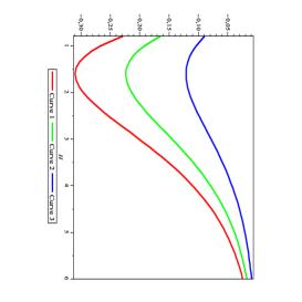
Figure 1: $q$-deformed magnetization as a function of magnetic field $H$ for $q=0.1$ (blue), $q=0.5$ (green), $q=0.99$ (red).

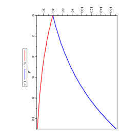
Figure 2: $C^{*}$ as a function of the number of dimensions for $L_{-}=2\pi-0.9$ (red), $L_{+}=2\pi+0.9$ (blue), $\lambda=1$.

IV Conclusions

We apply the $q$-deformed quantum algebra in the Landau diamagnetism problem embedded in $D$-dimensions, in the limit of high temperatures. We obtain $q$-deformed values $q\neq 1$ for internal energy, number of particles, magnetization, susceptibility and specific heat. We see that the q-deformed thermodynamical quantities change, except the specific ones, i.e., those quantities per particles, such as specific heat. That means that all effect of the q-deformation is completely stored into the number of particles $N$. It seems to be related to impurities in a sample of a diamagnetic material. As expected, in the limit $q=1$ we see that the results are identical to those in the literature patt ; hua . The thermodynamical quantities also depend on the number of $D$-dimensions since it is present in the constant $C^{*}\propto\left(\frac{L}{2\pi\lambda}\right)^{D}4\pi^{2}\lambda^{2}$ — see Fig. 2. Note that for $L<2\pi\lambda$ this constant decreases as the number of dimensions $D$ increases. On the other hand, $C^{*}$ increases with $D$ as $L>2\pi\lambda$, and has no changes as $L=2\pi\lambda$. An interesting phenomenon, for instance, can be achieved in the second case (the bulk sample is larger than the thermal wavelength $\lambda$), where the the magnetization is minimized for $D=3$ (we are assuming all times $D\geq 3$). On the other hand, in the first case (the bulk sample is smaller than the thermal wavelength $\lambda$) the magnetization is minimized just for a large number of dimensions. This suggests a mechanism that can be used to select the maximal number of dimensions of the spacetime with minimal diamagnetism, as in our Universe. This fact may find some applications in extra-dimensional physics such as modern cosmology, particle physics and string theory.

- (1) L.C. Biedenharn and M.A. Lohe, Quantum Group Symmetry and Q-Tensor Algebras, (World Scientific, Singapore, 1995).
- (2) F. Wilczek, Fractional Statistics and Anyon Superconductivity, (World Scientific, Singapore, 1990) and references therein.
- (3) M. Chaichian, R. Gonzales Felipe, C. Montonen, J. Phys. A. Math. Gen. 26, 4017 (1993).
- (4) D. Galetti, Braz. J. Phys. 33, 1 (2003).
- (5) L. Biedenharn, J. Phys. A: Math. Gen. 22, L873 (1989).
- (6) A. Macfarlane, J. Phys. A: Math. Gen. 22, 4581 (1989).
- (7) F. Jackson, Mess. Math. 38, 57 (1909).
- (8) H. Exton, q-Hypergeometric Functions and Applications, (John Wiley and Sons, New York, 1983).
- (9) E.G. Floratos, J. Phys. Math. 24, 4739 (1991).
- (10) A. Lavagno, A.M. Scarfone and N.P. Swamy, J. Phys. A: Math. Theor. 40, (2007) 8635-8654.
- (11) C. Tsallis, J. Stat. Phys. 52, 479 (1988); E.M. Curado and C. Tsallis, J. Phys. A: Math. Gen. 24, L69 (1991); C. Tsallis, R.S. Mendes and A.R. Plastino, Physica A 261, 534 (1998).
- (12) S. Abe, Phys. Lett. A 224, 326 (1997).
- (13) G. Kaniadakis, Phys. Rev. E 66, 056125 (2002).
- (14) G. Kaniadakis, M. Lissia and A.M. Scarfone, Physica A 340, 41 (2004); G. Kaniadakis, M. Lissia and A.M. Scarfone, Phys. Rev. E 71, 046128 (2005).
- (15) A. Lavagno and N.P. Swamy, Phys. Rev. E 61, 1218 (2000); A. Lavagno and N.P. Swamy, Phys. Rev. E 65, 036101 (2002).
- (16) A. Erzan, Phys. Lett. A 225, 235 (1997).
- (17) G. Bimonte, C. Esposito, G. Marmo and C. Stornaiolo, Phys. Lett. A 318, 313 (2003).
- (18) Y.J. Ng, J. Phys. A 23, 1023 (1990).
- (19) J.J. Sakurai, Modern Quantum Mechanics, (Addison Wesley Reading, Mass., 1994).
- (20) R.J. Finkelstein, Int. J. Mod. Phys. A 13, 1795 (1998).
- (21) R.K. Pathria, Statistical Mechanics, Pergamon Press, Oxford (1972)
- (22) K. Huang, Statistical Mechanics, John Wiley & Sons, (1987).
- (23) R. Thompson and D.J. Morton, J. Sedim. Petrology 49, 0801 (1979).