Spin-polarization effects in the processes of synchrotron radiation and electron-positron pair production by a photon in a magnetic field

Abstract

Spin and polarization effects and correlations between them in the processes of pair production by a photon and synchrotron radiation in a magnetic field are considered. Expressions for the probabilities of the processes with arbitrary polarizations of the particles are obtained. These expressions are analyzed in detail in both the Lowest Landau Levels and ultrarelativistic approximations.

I Introduction

The study of the quantum-electrodynamic processes involving photons and electrons in strong external electromagnetic fields is still topical from both an experimental and theoretical point of view, despite an extensive literature on this subject. The first relativistic theory of the processes of synchrotron radiation and pair production in a magnetic field was investigated in the works Klepikov -FIAN in the approximation of ultrarelativistic motion of particles. The results of these works are included in the monographs of Sokolov and Ternov Sokolov1 , Sokolov2 . The operator method for solving this problem was applied by Baier and Katkov in the quasiclassic ultrarelativistic case Baier1 ; Baier2 . Recently, there has appeared the work of these authors BaierAr , where the operator method was used to study the process of electron-positron pair production by a photon, when the particles are located at low-energy Landau levels. In the Ref. Herold , synchrotron radiation of electron-positron plasmas has been studied and Landau level splitting due to interaction with photon field is taken into account. In the Ref. Preece , the influence of electron spins on radiation probability for the first 500 levels has been considered. Reference Pavlov is devoted to the studying of radiative width of cyclotron line and level splitting due to interaction with QED-vacuum. We also mention Refs. Schwinger -Semionova , where the processes of photon radiation and pair production was considered for the case of polarized particles. It should be noted that correlations between spin and polarization effects in these processes have not been studied in detail yet.

The purpose of this paper is theoretical research of spin and polarization effects and their correlation in the processes of synchrotron radiation and pair production by a photon in a strong magnetic field. We use general expressions for probability of the processes when spin projections of the particles and photon polarization are arbitrary. In this paper the Stokes parameters are used to define photon polarization. Expressions for the probabilities are analyzed in the ultraquantum (Lowest Landau Levels) and the ultrarelativistic approximations that are most important for experimental applications. In these approximations, simple analytical expressions depending on both particles’ spins and photon polarization were obtained. Thus, it turned out to be possible to carry out analysis of spin and polarization effects and correlations between them.

Carrying out of corresponding experiments implies usage of magnetic fields that are comparable with the critical Schwinger one $B_{c}=m^{2}c^{3}/e\hbar\approx 4.41\cdot 10^{13}$ G and are not feasible in terrestrial laboratories. The greatest constant field obtained is about $100$ T Maglab and the greatest pulse field is $\sim 10^{6}$ G Arzamas . Nevertheless, we should point out the possibility to obtain a strong magnetic field on QED length of about $10^{-11}$ cm PAST . In heavy ion collisions Darmstadt (Darmstadt, GSI) Coulomb fields compensate and the magnetic field can reach a strength of $10^{12}$ G in the region between ions if the impact parameter is about $10^{-11}$ cm. In principle, QED processes can be observed in this region.

The investigation of the QED processes keeps actuality and great importance in view of existence of strong magnetic fields around neutron stars Harding6 . Particularly, cyclotron lines have been found in the radiation of X-ray pulsars. These lines correspond to the cyclotron radiation (absorption) of electrons that occupy the lowest Landau levels. A lot of works are devoted to the investigation of these lines Bussard -Harding4 . References Baring1 -Thompson considering the pair production process and its applications to the pulsars are worth mentioning too.

It should be noted that the astrophysical modeling of pulsars implies that radiation is emitted by unpolarized particles. However, electron-positron plasma in the magnetosphere of a pulsar is mostly created by the pair production process. Consequently, electron spins in Landau levels are not equally populated. In Section IV we compare transition rates for the cases of polarized and unpolarized particles.

II Spin-polarization effects in the process of synchrotron radiation

In a uniform, homogenous magnetic field $B^{\prime}=B/B_{c}$ energy levels of electrons are

$$E_{n}=\sqrt{p_{z}^{2}+m^{2}+2lB^{\prime}m^{2}}$$ (1)

where $l$ is the principal quantum number ($l=0,1,2...$), and $p_{z}$ is the momentum component parallel to the field (we will use natural units, where $\hbar=c=1$ throughout). In each Landau state, the electron may have spin-up ($s=+1$) or spin-down ($s=-1$) along the field direction, except in the ground state, where only the spin-down state is allowed.

The procedure of obtaining the probabilities of first-order processes is well known and we omit the corresponding calculations. The resulting expressions for probabilities of the processes of synchrotron radiation and pair production that depend on particles’ spins as well as on photon polarization are given in the appendixes. Now let us proceed directly to the analysis of the probabilities.

II.1 Ultraquantum approximation

In the Lowest Landau Levels (LLL) approximation, intensity distribution of synchrotron radiation is presented by the expressions (24)–(27).

The ”no spin-flip” processes have the greatest probability because they have the lowest power of the small parameter ${B^{\prime}\ll 1}$. Moreover, due to the condition $l>l^{\prime}$ the radiation probability is maximal for the process with particle spins directed against the field. The energetically unfavorable process with particles polarizations $s=1$, $s^{\prime}=-1$ has the smallest probability. Process probability decreases as $(B^{\prime})^{l-l^{\prime}}$ if the difference $l-l^{\prime}$ increases therefore the transition $l\to l-1$ is the most probable.

The ”no spin-flip” processes have identical dependence of probability on the Stokes parameters. Probability of the energetically favorable spin-flip process (26) differs in the sign of the Stokes parameter $Q$, therefore radiation has opposite linear polarization for spin-up – spin-down transitions.

Let us consider two opposite cases of linear photon polarization. If the polarization vector is perpendicular to the vector of a magnetic field $\vec{B}$ then the Stokes parameter $Q$ equals $-1$, $Q=-1$. Hereafter we will call it perpendicular photon polarization. If the polarization vector belongs to the same plane as the wave vector $\vec{k}$ and the vector $\vec{B}$ then equation $Q=1$ is true and such polarization is called parallel polarization.

In the case of parallel polarization ($Q=1$) the probability of radiation equals zero in the direction perpendicular to the field ($\theta=\pi/2$) for the processes without flip of spin. Probability of the spin-down–spin-up transition (27) is minimal in this direction. Probability of the other spin-flip process is a slowly varying function of the polar angle. In the case of perpendicular polarization ($Q=-1$) radiation is absent in the direction $\theta=\pi/2$ for the spin-flip processes, but probabilities of the transitions without flip of spin depend on the polar angle weakly.

Radiation has circular polarization in the direction along the magnetic field, since the probability does not depend on the parameter of linear polarization $Q$ if the condition $\cos\theta=\pm 1$ is fulfilled. If the photon has right circular polarization ($Q=1$), radiation probability is maximal in the direction along the magnetic field ($\theta=0$) and equals zero in the direction against the field. In the case of left polarization ($Q=-1$), the situation is reversed.

One can see that the polarization of radiation is the same as in the case of classical motion of an electron. As follows from the above, substantial spin-polarization correlation takes place. The shape of the angular distribution of radiation probability and its representative values are determined by the values of photon polarization and spin projections of the particles.

The angular distributions of intensity in relative units for linear polarization of the radiated photon (the transition from the level $l=2$ to $l^{\prime}=1$ is chosen as an example) are shown in Fig. 1 and can be expressed as:

$$\iota=\frac{dI/du}{\iota_{0}},$$

where $\iota_{0}=\alpha(B^{\prime})^{3}(mc^{2})^{2}/4\hbar$ and equals to $\sim 10^{9}$ erg/s for the field $B^{\prime}=0.1$ ($\alpha$ is the fine structure constant).

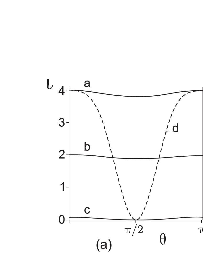
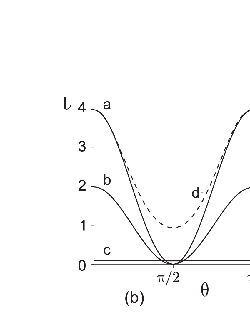
Figure 1: Angular distribution of the radiation intensity of perpendicular (a) and parallel (b) linear polarization. The value of the field is $B^{\prime}=0.1$. Here: (a) spin-down–spin-down transition; (b) spin-up–spin-up transition; (c) $s=1$, $s^{\prime}=-1$; (d) $s=-1$, $s^{\prime}=1$ (broken line). The right scale relates to the dashed line (d).

Let us estimate radiation intensity by the order of magnitude in two cases. Some of the neutron stars have a surface magnetic field around $B\sim 10^{12}$ G ($B^{\prime}=0.1$). In such field radiation intensity has the order of magnitude of $\sim 10^{9}$ erg/s in the no spin-flip processes. In the case of energetically favorable spin-flip process ($s=1$, $s^{\prime}=-1$) intensity is lower by a factor of 10. In the other spin-flip process ($s=-1$, $s^{\prime}=1$) intensity is lower by a factor of 1000. The ratio between intensities for the spin-flip and no spin-flip processes is about 5 %. This result is well known from the number of works (see, for example Bagrov , RQT ). Intensity decreases exponentially if the field becomes lower. For example, in the case of white dwarfs (field strength is $B\sim 10^{8}$ G and $B^{\prime}\sim 10^{-5}$ ) intensity is about $\sim 10^{-3}$ erg/s and the above ratio is $\sim$10^-3 %.

II.2 Ultrarelativistic approximation

In the ultrarelativistic case radiation intensity defined by Eq. (28)

$$\frac{d^{2}I^{ss^{\prime}}}{dyd\Psi}=I_{0}\frac{9}{8\pi^{2}}\frac{y^{2}F^{2}}{\left({2+z}\right)^{3}\left({2+z\left({1-y}\right)}\right)^{2}}D^{ss^{\prime}},$$ (2)

where $z=3hE/m$, $E$ is the initial electron energy, $y=\omega(2+z)/Ez$, $F=\sqrt{1+\Psi^{2}}$, $\Psi=\psi/\psi_{c}$, $\psi=\pi/2-\theta$. Factors $D^{ss^{\prime}}$ are given by Eqs.(29)-(32).

Angular distribution of radiation intensity is symmetrical with respect to the orbit plane if photon polarization is linear. Indeed, when $V=0$, $Q=-1$ (perpendicular polarization) Eqs. (29) – (32) take on the following form:

$$D^{++}=2y^{2}z^{2}\left({\sqrt{\frac{a}{b}}FK_{2/3}-K_{1/3}}\right)^{2},$$ (3)

$$D^{--}=2y^{2}z^{2}\left({\sqrt{\frac{a}{b}}FK_{2/3}+K_{1/3}}\right)^{2},$$ (4)

$$D^{-+}=D^{+-}=2y^{2}z^{2}\Psi^{2}K_{1/3}^{2}.$$ (5)

Symmetry about the plane $\psi=0$ takes place since the above expressions depend only on the square of the angle $\psi^{2}$. One can see that inequality $D^{--}>D^{++}$ is always true. Thus, radiation intensity is greater if particles are in a spin-down state. It is clear because this state is energetically favorable. Intensities of the spin-flip processes are equal and radiation is absent in the perpendicular to the field direction ($\psi=0$). Radiation intensity considerably decreases if electron spin flips.

In the case of parallel polarization, the expressions (29) – (32) have the form

$$D^{++}=D^{--}=2\Psi^{2}aK_{1/3}^{2},$$ (6)

$$D^{-+}=2y^{2}z^{2}\left({FK_{2/3}-K_{1/3}}\right)^{2},$$ (7)

$$D^{+-}=2y^{2}z^{2}\left({FK_{2/3}+K_{1/3}}\right)^{2}.$$ (8)

As follows from Eq. (6), intensities of no spin-flip processes coincide. They vanish in the perpendicular to magnetic field direction ($\psi=0$). Intensity of the energetically unfavorable spin-flip process is minimal in this direction. Symmetry about the plane $\psi=0$ takes place too.

As follows from Eqs. (3) – (8), in general, intensity of the spin-flip process (8) is comparable with intensity of the most probable one (4). Indeed, the ratio between the differential intensities is equal to the value $D^{+-}/D^{--}$. In the case of large photon frequency ($\omega\rightarrow E$), the condition $\sqrt{a/b}=(E+E^{\prime})/\omega\rightarrow 1$ is true. Consequently, $D^{+-}/D^{--}\rightarrow 1$. On the other hand, in the case of low photon frequency ($\omega\ll E$) $\sqrt{a/b}\gg 1$ and we obtain the well-known result $D^{+-}\ll D^{--}$ Bagrov . This effect is significant when $z\gtrsim 1$, since the maximum of radiation intensity shifts into the region of high frequency as the parameter $z$ increases. The same result was obtained numerically in Ref. Preece .

The dependence of differential intensity on the output angle and photon frequency in the case of linear polarization of radiation is shown in Fig. 2.

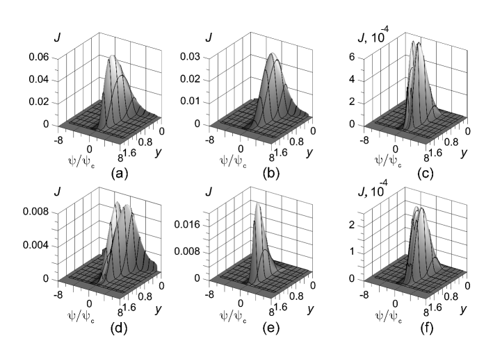
Figure 2: Dependence of intensity on the output angle and photon frequency in the case of perpendicular (a)–(c) and parallel (d)–(f) linear polarization of the photon: (a) $s=s^{\prime}=-1$; (b) $s=s^{\prime}=1$; (c) spin-flip processes; (d) spins of the same orientation; (e) $s=1,s^{\prime}=-1$; (f) $s=-1,s^{\prime}=1$. Here, $J=I/I_{0}$, $z=3EB^{\prime}/m=3$.

The following result should be mentioned. It is known that relativistic particles emit radiation into a narrow cone in the line of motion and intensity is maximal in the direction of velocity. However, intensity of perpendicular polarized radiation is zero in the direction $\psi=0$ if flip of spin occurs. Parallel polarized radiation is absent in this direction for the no spin-flip processes. Although this effect is unexpected in the ultrarelativistic approximation, it has general origin. Indeed, in the LLL approximation, radiation in the line of motion is absent in the same cases as in the ultrarelativistic approximation.

Angular intensity distribution of circular polarized radiation is not symmetrical in respect to the plane $\psi=0$. Intensity of radiation of right circular polarization is maximal in the region $\psi>0$ and intensity of the left circular polarized radiation is maximal in the region $\psi<0$.

In general, the process of synchrotron radiation has similar features in the ultrarelativistic and the LLL approximations. In the LLL approximation intensity is maximal along the field direction ($\psi=\pi/2$) if polarization is right circular. In the ultrarelativistic approximation the maximum of right polarized radiation is shifted into the region $\psi>0$. The shift of the maximum becomes greater if frequency of the radiated photon decreases. It is clear since angular distribution of radiation passes to the classical one in the limit case of small frequency. The situation is reversed if polarization of radiation is a left circular one.

Note that in the ultrarelativistic approximation intensity depends on the parameter $z$ only. This parameter is defined by a product of the energy of the initial electron and the parameter of magnetic field $B^{\prime}$: $z=3EB^{\prime}/m$. Let us estimate intensity of radiation. Let $B^{\prime}=10^{-5}$ and $E\sim 50$ GeV. In this case $z=3$ and radiation intensity per unit of frequency can be estimated at $\sim 10^{-9}$ erg.

III Spin-polarization effects in the pair production process

Probability of the pair production process contains a denominator that goes to zero if the pair produced with zero longitudinal momenta, i.e. at the reaction threshold. It results in the occurrence of divergences and the process is a resonant one (Fig. 3).

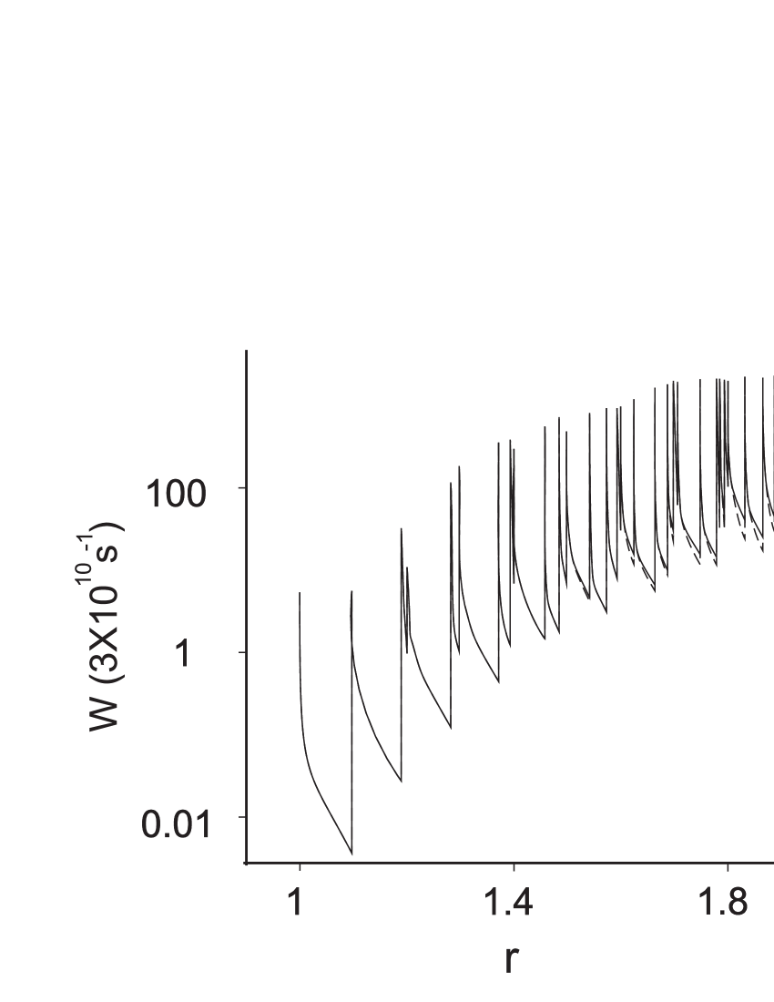
Figure 3: Dependence of total probability of the pair production process on the parameter $r=\omega^{2}/4m^{2}$. Broken line depicts the result of the Ref. BaierAr .

Enough attention has been paid to the explanation of the physical nature of these divergences, for example, in Ref.  Graziani , but there is not a complete clarity in understanding of this matter. In our opinion, the presence of singularities is associated with neglected emission of soft photons, which always accompanies quantum-electrodynamics processes. This phenomenon is similar to the so-called “infra-red catastrophe” of the bremsstrahlung process at the scattering by a Coulomb center Fomin (see Fig. 4). It is known, that infra-red divergences arise so far as the perturbation theory becomes incorrect for soft photon emission.

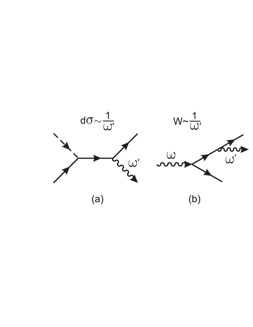
Figure 4: Feynman diagrams of the processes: (a) bremsstrahlung at the scattering by a Coulomb center and (b) pair production with radiation of a final photon. Both probabilities contain the same divergence at $\omega^{\prime}\to 0$

A cross section of the bremsstrahlung process is in inverse proportion to the frequency of the final photon: $d\sigma\sim 1/\omega^{\prime}$. The cross section becomes unrestrictedly large if the frequency converges to zero. Probability of the pair production process has similar dependence on frequency if an additional final photon is taken into account. In this case, the divergence at the threshold (longitudinal momentum is zero) vanishes Fomin .

III.1 LLL approximation

First of all, obtained probability of pair production (39) – (42) does not depend on the Stokes parameter $V$ that defines circular polarization. This fact is a result of the choice of the reference frame where the wave vector of a photon belongs to the classical orbit plane. Moreover, probability does not depend on the parameter $U$ too. This parameter defines polarization in the directions that make angles of $\pm\pi/4$ with the vector of the magnetic field. However these directions are equivalent since there is the single preferential direction of vector $\vec{B}$ in the plane perpendicular to $\vec{k}$.

When an electron and a positron are produced in the low spin state ($s=-1$, $s^{\prime}=1$) the process has the greatest probability because the corresponding expression (41) contains the small parameter $B^{\prime}$ in the lowest power. In the cases $s^{\prime}=1$, $s=1$ and $s^{\prime}=-1$, $s=-1$ the expressions of probability (39), (40) differ from Eq. (41) in the sign of the parameter of linear polarization $Q$. It should be noted that the similar effect takes place in the process of synchrotron radiation. If particles are created in the energetically high spin state ($s=1$, $s^{\prime}=-1$), the process has the smallest probability.

We may assign an arbitrary value for polarization of the initial photon because it is defined by the initial conditions of the problem. When $Q=-1$ probability of the pair production vanishes in the energetically low spin state $s=-1$, $s^{\prime}=1$ (41). It is necessary to calculate the probability $W^{-+}$ in the next order in small parameter $B^{\prime}$ before comparison of values of the probabilities. After the corresponding calculations probability $W^{-+}$ takes on the following form:

$${\begin{array}[]{l}W^{-+}=\displaystyle\frac{\alpha m^{3}A}{2\omega}\frac{B^{\prime}}{p_{z}g}(1+Q)\times\\ \times\displaystyle\left[1+\frac{1}{2}B^{\prime}\left(3\left(l+l^{\prime}\right)-2\frac{ll^{\prime}}{g^{2}}\right)\right],\\ \end{array}}$$ (9)

where $g=1+\left({p_{z}/m}\right)^{2}$. One can see that dependence of the probability on polarization remains the same as in the previous case. Thus, the greatest probabilities are $W^{++}$ and $W^{--}$ in the case of perpendicular polarization ($Q=-1$).

As follows from above, substantial correlation between polarization of the initial photon and spin projections of produced particles takes place. Therefore produced particles are polarized. Let us find the polarization degree of electrons. By definition, it has the form

$$P_{-}=\frac{W^{+}-W^{-}}{W^{+}+W^{-}},$$ (10)

where $W^{+}=W^{++}+W^{+-}$ and $W^{-}=W^{-+}+W^{--}$. The probability $W^{+-}$ is the smallest one by its order of magnitude and can be neglected:

$$P_{-}=\frac{W^{++}-W^{-+}-W^{--}}{W^{++}+W^{-+}+W^{--}}.$$ (11)

If $Q\neq-1$, the contribution $W^{-+}$ exceeds all other terms, therefore $W^{++}$ and $W^{--}$ can be neglected. Consequently,

$$P_{-}\approx-1.$$ (12)

Hence, the spins of produced electrons are almost completely oriented against the field direction if the condition $Q\neq-1$ is fulfilled. In order to find the more accurate expression of the polarization degree we have to substitute Eqs. (39), (40) and (9) into Eq.(11) and expand $P_{-}$ in a power series in the first order in small parameter $B^{\prime}$. After simple calculations, the polarization degree takes on the form

$$P_{-}=-1+B^{\prime}l\frac{1-Q}{1+Q}.$$ (13)

In the case $Q\to-1$, the quantity $W^{-+}$ in the expression (11) can be neglected and

$$P_{-}=\frac{l-l^{\prime}}{l+l^{\prime}}.$$ (14)

Consequently, the polarization degree depends on the numbers of Landau levels of an electron and a positron. The degree of polarization is equal to zero when the condition $l^{\prime}=l$ is fulfilled. In the general case the inequality $|P_{-}|\leq 1$ is true. Consequently, produced electrons are always partially polarized if $l^{\prime}\neq 0$.

The process has the maximal probability when an electron and a positron are produced at close or the same Landau levels, therefore polarization degree converges to zero if the Landau level numbers increase.

Thus, the degree of particle polarization is determined by polarization of the initial photon. Linear polarization can be changed from a perpendicular one to a parallel one by rotation of a photon beam by the angle $\pi/2$ about the beam axis. It causes substantial changing of the number of particles in the spin-up and spin-down states. Thus, it is possible to control the spin orientation of new particles rotating the photon beam.

Note that the averaged over photon polarization and summed over particles’ spins total probability is in agreement with results of previous works (Fig. 3) BaierAr , Harding1 . A discrepancy between our result and the computations of Baier and Katkov is associated with violation of the conditions of LLL approximation.

III.2 Ultrarelativistic approximation

In the ultrarelativistic case probability of pair production is given by Eq.(43):

$$W^{ss^{\prime}}=\int\limits_{0}^{\Omega}{\int\limits_{-\infty}^{\infty}{W_{0}\frac{F^{2}D^{ss^{\prime}}}{24\pi^{2}\Omega\varepsilon^{2}\left({\Omega-\varepsilon}\right)^{2}}d\varepsilon d\Psi}},$$ (15)

where $\Psi=p_{z}/E$, $\Omega=B^{\prime}\omega/m$, $\varepsilon=B^{\prime}E/m$, $E$ is the electron energy, and $D^{ss^{\prime}}$ are defined by Eqs.(44) – (47).

When the photon is perpendicular polarized the factors $D^{ss^{\prime}}$ (44) – (47) have the following forms:

$$D^{-+}=D^{+-}=2\Psi^{2}K_{1/3}^{2},$$ (16)

$$D^{++}=2\Omega^{2}\left({F\frac{\rho}{\Omega}K_{2/3}-K_{1/3}}\right)^{2},$$ (17)

$$D^{--}=2\Omega^{2}\left({F\frac{\rho}{\Omega}K_{2/3}+K_{1/3}}\right)^{2}.$$ (18)

In the case of parallel photon polarization (${Q=1}$), we obtain

$$D^{-+}=2\Omega^{2}\left({FK_{2/3}-K_{1/3}}\right)^{2},$$ (19)

$$D^{+-}=2\Omega^{2}\left({FK_{2/3}+K_{1/3}}\right)^{2},$$ (20)

$$D^{++}=D^{--}=2\rho^{2}\Psi^{2}K_{1/3}^{2}.$$ (21)

The expressions (16) – (21) depend on the square of the angle $\psi^{2}$ only if polarization of the photon is linear. Consequently, angular distribution of the probability is symmetrical with respect to the orbit plane $\psi=0$.

As follows from Eq.(16), in the case of perpendicular photon polarization, the probabilities of the processes with opposite particles’ spins are equal to each other. The probabilities $W^{+-}$ and $W^{-+}$ vanish if the longitudinal momenta of the particles are zero. If the particles have spins of the same orientation then the corresponding probabilities $W^{++}$ and $W^{--}$ are mirror reflections of each other in the plane $E=E^{\prime}$. Indeed, after the replacement $E\leftrightarrows E^{\prime}$ the argument of the McDonald functions $X_{p}={\omega F^{3}}/({3EE^{\prime}})$ does not change and the quantity $\rho/\Omega=({E-E^{\prime}})/\omega$ changes its sign.

In the case of parallel polarization, the probabilities $W^{++}$ and $W^{--}$ are equal to each other and vanish if the angle $\psi$ goes to zero. These probabilities also vanish if the energies of the electron and the positron are equal ($E=E^{\prime}$), since $\rho=B^{\prime}\left({E-E^{\prime}}\right)/m=0$ in this case. One can see from Eqs. (19), (20) that the probability $W^{+-}$ is greater than $W^{-+}$ since the factor $D^{+-}$ is a square of a sum of nonnegative summands and the factor $D^{-+}$ is a square of a difference of the same terms. Thus, production of particles in the energetically high spin state ($s=1$, $s^{\prime}=-1$) is more probable than production in the lower state ($s=-1$, $s^{\prime}=1$). Note that in the LLL approximation, the situation is reversed.

It is essential to note that in the cases mentioned above (16) and (21), the process is impossible if longitudinal momenta of particles are zero ($\Psi=p_{z}/E=0$). On the contrary, in the case of unpolarized particles, probability goes to infinity if the longitudinal momenta of particles vanish (Fig. 3).

Dependence of the process probability on the electron energy and output angle is shown in Fig. 5. Photon polarization is assumed linear and the value of the parameter $\Omega=\omega B^{\prime}/m$ is 1.

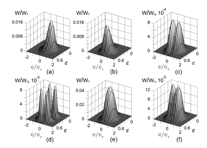
Figure 5: Dependence of probability of pair production by a photon of perpendicular polarization (a)–(c) and parallel polarization (d)–(f) on the electron energy and output angle: (a) $s=s^{\prime}=1$; (b) $s=s^{\prime}=-1$; (c) spins of opposite orientations; (d) spins of the same direction; (e) $s=1,s^{\prime}=-1$; (f) $s=-1,s^{\prime}=1$. Here, $W_{0}=\alpha mB^{\prime}$, $\varepsilon=EB^{\prime}/m$, $\psi_{c}=1/\sqrt{2lB^{\prime}}$, $\Omega=\omega B^{\prime}/m=1$.

As follows from the Eqs. (28) – (32), if a photon has circular polarization, then maximum of probability is shifted with respect to the plane that is perpendicular to the magnetic field ($\Psi=0$), and cases of right and left polarizations differ by the shift direction only.

Integration of the expressions (44) – (47) over the electron energy $\varepsilon$ and the output angle $\Psi$ gives the total probability of the pair production process. The dependence of the total probability of the process with polarized particles on the parameter $\lambda=4/3\Omega=4m/3\omega B^{\prime}$ is shown in Fig. 6. Photon polarization is assumed to be linear.

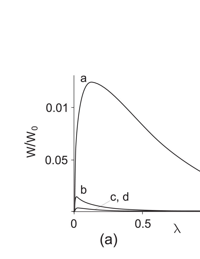
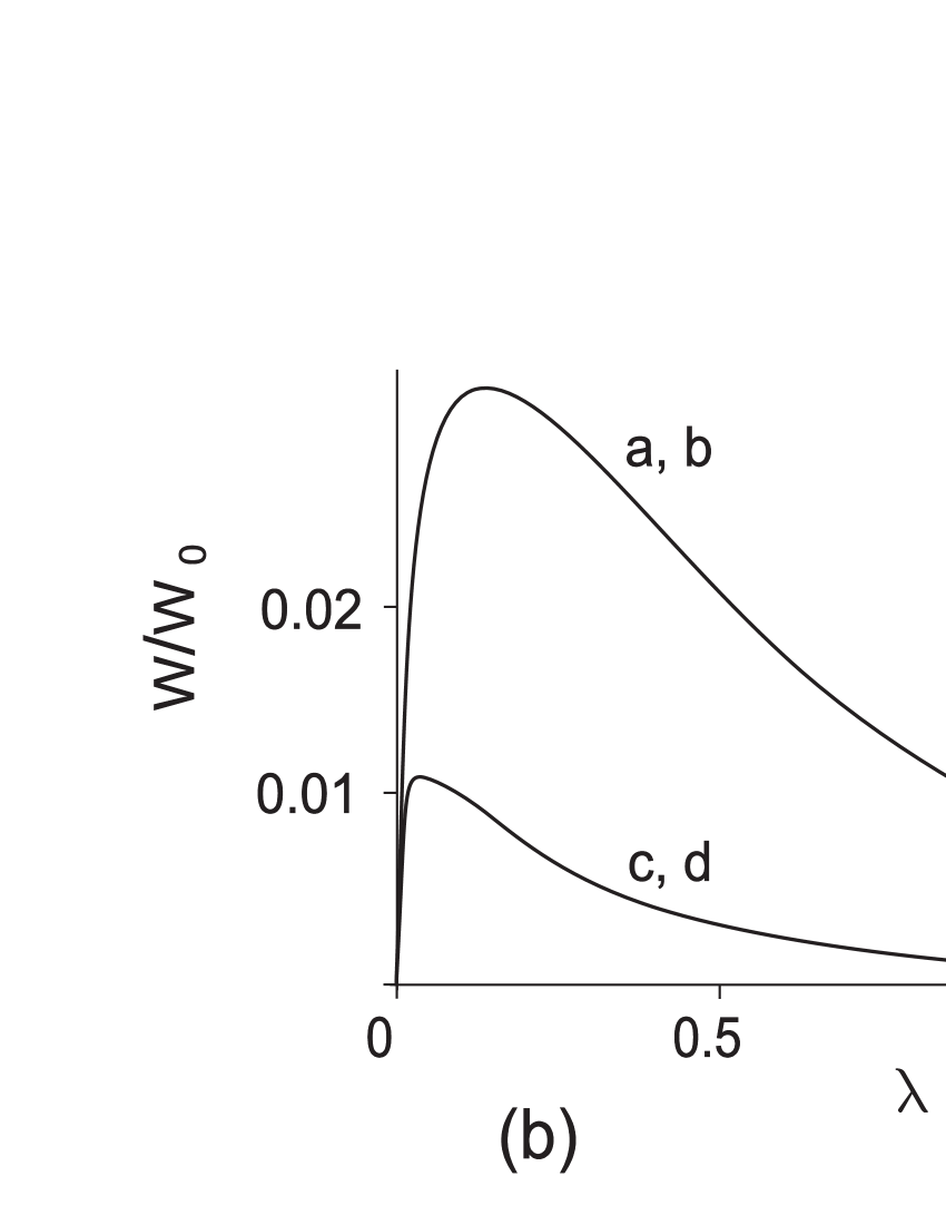
Figure 6: The dependence of total probability of pair production on the parameter $\lambda=4/3\Omega$. (a) perpendicular photon polarization; (b) parallel photon polarization. (a) energetically high spin state of produced particles; (b) energetically low spin state; (c), (d) spins of the same direction.

One can see that probabilities coincide if particles are produced with spins of the same orientation. It is clear from the analysis of expressions (17), (18), (21).

As opposite to the case of the LLL approximation, the process has the largest probability when a pair is produced in the high spin state ($s=1$, $s^{\prime}=-1$) by a photon of parallel polarization ($Q=1$). In this case, electron spins are almost entirely oriented along the field and positron spins are oriented against the field.

In the case of perpendicular polarization, the probabilities also coincide if particles’ spins have opposite directions. Thus, the beam of produced particles is unpolarized. As mentioned above, in the LLL approximation, the polarization degree of electron spins (14) converge to zero as the numbers of Landau levels increase. It is in agreement with the obtained result.

Finally, it can be concluded that in the ultrarelativistic approximation one can control the polarization degree by the setting of the photon polarization as well as in the LLL approximation.

IV Application

The obtained results can be applied to astrophysical modeling of pulsars. According to current pulsar models, high energy photons produce electron-positron pairs in the pulsar magnetic field that subsequently synchrotron radiate. Particles are considered as unpolarized. However, as follows from Eqs. (12), (14) produced electrons have certain polarization that is defined by initial photon polarization. Thus, their synchrotron rates are different from the rates of unpolarized particles. Let us calculate the ratio $R$ between transition rates of polarized and unpolarized electrons.

IV.1 LLL approximation

Let $x_{+}$ be the fraction of spin-up electrons. After corresponding averaging of Eqs (24)-(27) the ratio $R$ will take the form

$$R=2\frac{l-x_{+}(l-l^{\prime})}{l+l^{\prime}}.$$ (22)

The fraction $x_{+}$ can be immediately obtained from Eqs. (39)-(42) with the assumption that the electron and the positron becomes created on the same energy level $l$:

$$x_{+}=\frac{1}{2}\frac{B^{\prime}l(1-Q)}{(1+Q)+B^{\prime}l(1-Q)},$$ (23)

where $Q$ is the polarization of the initial photon in the pair production process. One can see that $R=1$ when $x_{+}=1/2$. The ratio $R$ is greater than unity if $Q\neq-1$, and probabilities differ twice for ground state transitions and parallel polarization of the initial photon.

Figure 7(a) shows the dependence of the ratio $R$ on photon polarization and magnetic field strength for transition from $l=5$ to $l^{\prime}=0$. Figure 7(b) shows the dependence of the ratio $R$ on photon polarization and the number of final level. Field strength is $B^{\prime}=0.1$.

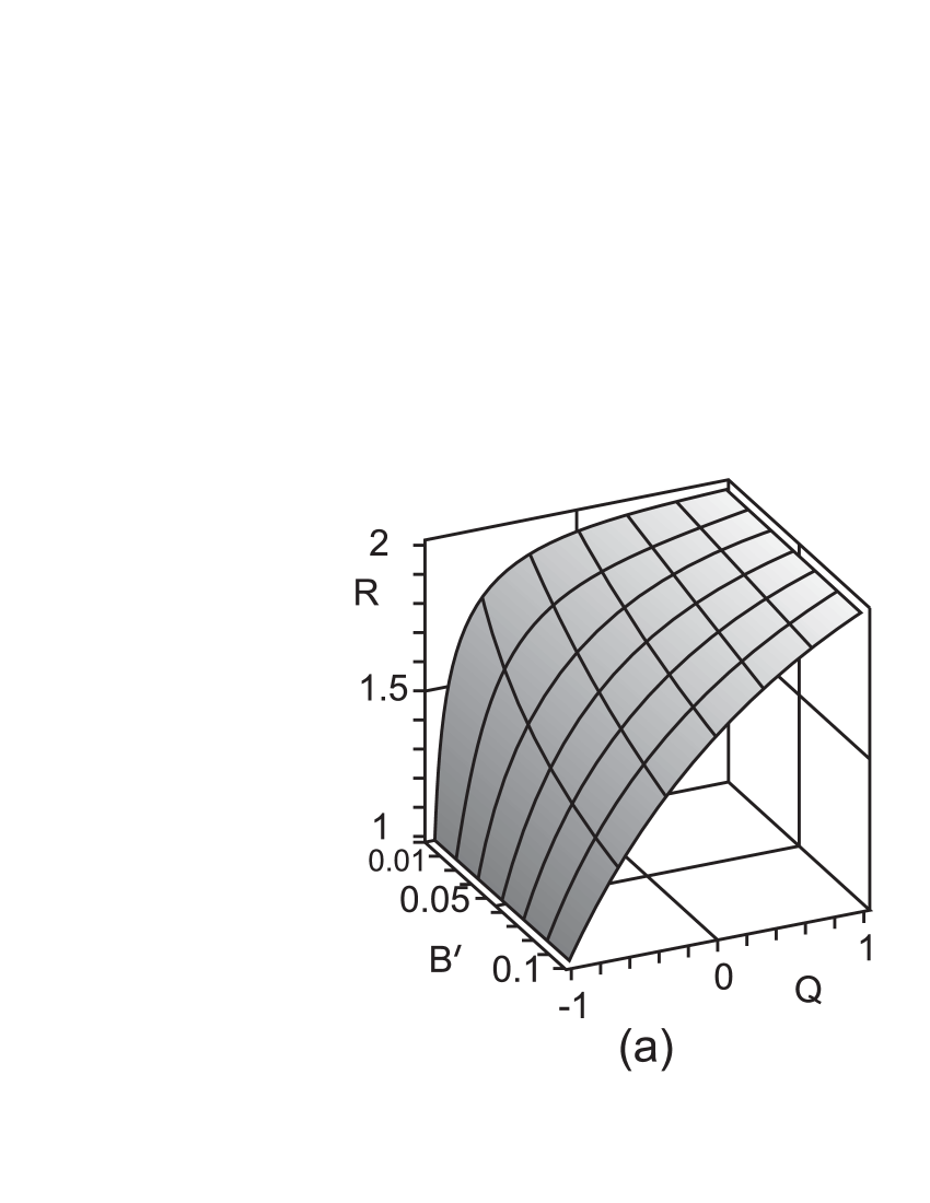
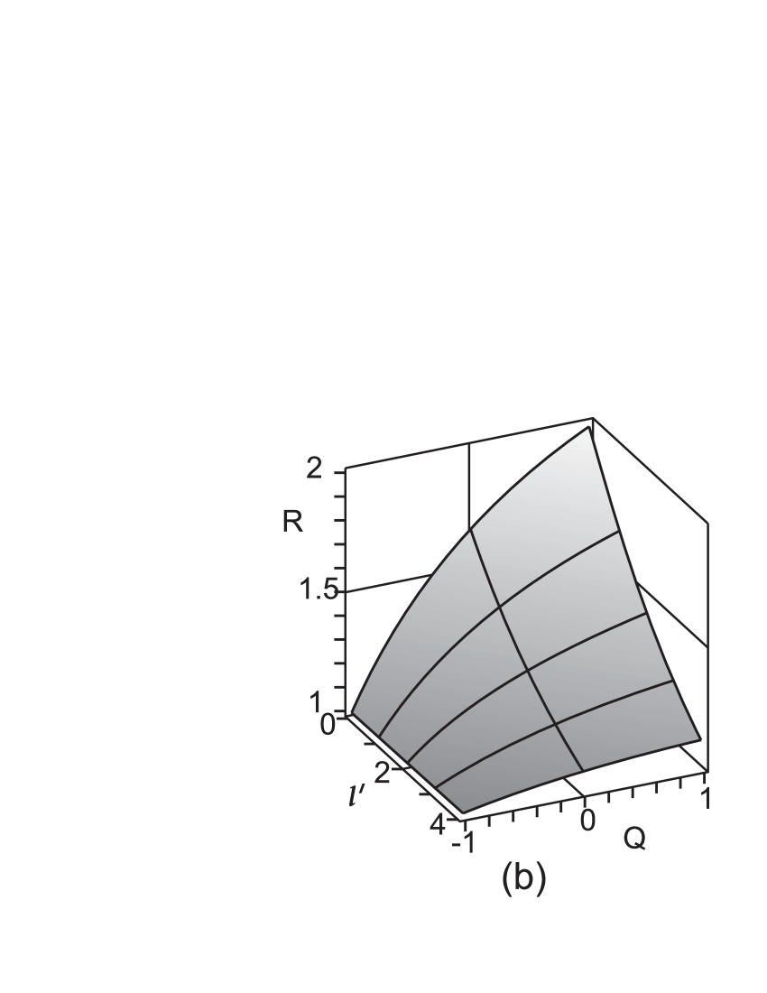
Figure 7: The dependence of the ratio $R$ between synchrotron rates of polarized and unpolarized electrons on: (a) photon polarization $Q$ and magnetic field $B^{\prime}$, $l=5$, $l^{\prime}=0$; (b) the number of final Landau level $l^{\prime}$ and photon polarization $Q$, $B^{\prime}=0.1$.

IV.2 Ultrarelativistic approximation

In ultrarelativistic approximation, the ratio $R$ can be obtained by the integration of Eqs. (28)-(32) and (43)-(47). In Fig. 8(a) the dependence of the ratio $R$ on initial photon polarization $Q$ and parameter $\Omega$ is shown. Initial photon frequency $\omega=100m$ is adopted and the magnetic field $B^{\prime}$ changes from value $B^{\prime}=0.001$ to value $B^{\prime}=0.1$. Figure 8(b) shows the dependence of the ratio $R$ on initial photon polarization $Q$ and final photon frequency $y=\omega/\omega_{c}$. The magnetic field is $B^{\prime}=0.1$.

One can see that $R\leq 1$ in this case. It has minimum value of about $0.86$ when $Q=1$ and goes to unit if $Q\rightarrow-1$.

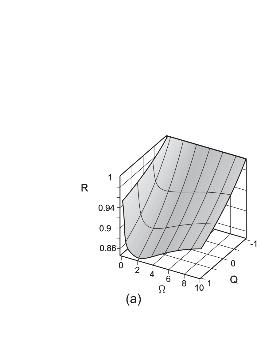
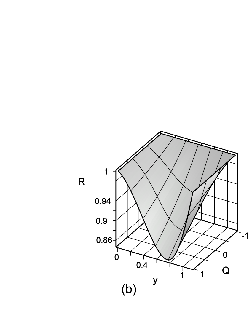
Figure 8: The dependence of the ratio $R$ between synchrotron rates of polarized and unpolarized electrons on: (a) initial photon polarization $Q$ and parameter $\Omega=\omega B^{\prime}/m$; (b) final photon frequency $y=\omega/\omega_{c}$ and initial photon polarization $Q$, $\Omega=10$.

Thus, it is substantial to take into account polarization-dependent spin bias.

V Conclusions

In the present work spin and polarization effects in the processes of synchrotron radiation and electron-positron pair photoproduction in a strong magnetic field have been considered. Spin projections and photon polarization have arbitrary values. Obtained expressions of probability have been analyzed in the ultrarelativistic and the LLL approximations.

Substantial correlation of spin and polarization effects takes place in the process of photon radiation. The dependencies of probabilities of no-flip processes on the Stokes parameter $Q$ are equal. Probability of spin-up–spin-down transition contains $Q$ with a reversed sign.

The processes without flip of spin are the most probable in the LLL approximation. Probability of these processes weakly depends on the polar angle $\theta$ in the case of perpendicular photon polarization. For parallel polarization, probability of radiation equals to zero in the direction $\theta=\pi/2$. In the ultrarelativistic approximation, the probability of the spin-flip process $s=1,s^{\prime}=-1$ is comparable with the probability of the most probable one if a high energy parallel polarized photon is radiated.

Radiation is absent in the perpendicular to magnetic field direction in the ultrarelativistic approximation too. Electrons radiate in a small interval in the vicinity of the orbit plane, but radiation intensity of perpendicular polarization is equal to zero in the direction $\theta=\pi/2$ when spin flips. In the case of the processes without flip of spin, radiation of parallel polarization is absent in this direction.

In the ultrarelativistic case, maximum of intensity of circular polarized radiation is shifted relative to the orbit plane. The shift of the maximum increases if the photon frequency decreases.

Probability of pair production depends on the parameter of linear polarization $Q$ only. Dependence on the other parameters can be eliminated by a choice of the reference frame.

Similar to the process of synchrotron radiation, essential spin-polarization correlation was found. In the LLL approximation, the process has the greatest probability when the pair is produced in the low spin state ($s=-1$, $s^{\prime}=1$). When spins of produced particles have the same orientation, process probability contains the Stokes parameter $Q$ with reversed sign.

In the ultrarelativistic case, probability of particle production with zero longitudinal momenta ($\Psi=p_{z}/E=0$) vanishes if particles have opposite spins and the photon has perpendicular polarization ($Q=-1$). If photon has parallel polarization ($Q=1$) then particles with spins of the same direction cannot be produced with zero longitudinal momenta. In contrast, in the case of unpolarized particles, probability becomes infinity if longitudinal momenta go to zero (Fig. 3).

On the contrary to the LLL approximation, pair production in the high spin state ($s=1$, $s^{\prime}=-1$) by the parallel polarized photon ($Q=1$) has the largest probability.

Produced particles may have preferred direction of their spins due to the spin-polarization effects. The degree of particle polarization is determined by polarization of the initial photon. In both considered approximations, particles are produced almost completely polarized if photon polarization is parallel, but the degree of particle polarization converges to zero in the case of photon of perpendicular polarization ($Q\to-1$).Thus, it is possible to control the spin orientation of new particles by rotating the plane of polarization of the photon beam.

The obtained results are applied to the modeling of pulsars. Synchrotron rates are compared in two cases: (a) electron spins are equally populated and (b) spin populations are determined by polarization of the initial photon that converts into electron-positron pairs. Radiation rates coincide for both cases when photon polarization is perpendicular. In the LLL limit case (a) exceed the other one twice if photon polarization is parallel. In the ultrarelativistic limit radiation intensity is greater in case (b) when photon polarization is parallel.

Appendix A Synchrotron radiation

We used the same expressions for the wave functions of an electron and a positron as in Ref. FominJETP . The reference frame where $p_{z}=0$ is chosen.

In the LLL approximation, probability of synchrotron radiation is given by the following expressions (the superscripts denote initial and final spin projections) Kholodov :

$$\frac{dW^{++}}{du}=\frac{1}{4}\alpha\Lambda^{2}B^{\prime}\omega\left({1+u^{2}+2uV-Q\left({1-u^{2}}\right)}\right),$$ (24)

$$\frac{dW^{--}}{du}=\frac{1}{4}\alpha\Lambda^{2}B^{\prime}\omega\frac{l}{l^{\prime}}\left({1+u^{2}+2uV-Q\left({1-u^{2}}\right)}\right),$$ (25)

$$\frac{dW^{+-}}{du}=\frac{1}{8}\alpha\Lambda^{2}(B^{\prime})^{2}\omega\frac{\left({l-l^{\prime}}\right)^{2}}{l^{\prime}}\left({1+u^{2}+2uV+Q\left({1-u^{2}}\right)}\right),$$ (26)

$$\begin{array}[]{l}\displaystyle\frac{dW^{-+}}{du}=\frac{1}{32}\alpha\Lambda^{2}(B^{\prime})^{4}\omega l\left({l-l^{\prime}}\right)^{2}\times\\ \times\left[{\left({1+u^{2}}\right)\left({1+L^{2}\left({1-u^{2}}\right)^{2}}\right)-2L\left({1-u^{2}}\right)^{2}+}\right.\\ +2Vu\left({1-L^{2}\left({1-u^{2}}\right)^{2}}\right)+\\ \left.{+Q\left({1-u^{2}+L^{2}\left({1-u^{2}}\right)^{3}-2L\left({1-u^{4}}\right)}\right)}\right],\\ \end{array}$$ (27)

Here, $\alpha$ is the fine structure constant, $l$ and $l^{\prime}$ are the numbers of initial and final Landau levels, $\omega$ is photon frequency, $V$ and $Q$ are the Stokes parameters, $L=(l-l^{\prime})/(l-l^{\prime}+1)$, $u=\cos\theta$ ($\theta$ is a photon polar angle), and

$$\Lambda=e^{-\frac{\eta}{2}}\eta^{\frac{l-l^{\prime}-1}{2}}\sqrt{\frac{\left({l-1}\right)!}{\left({l^{\prime}-1}\right)!}}\frac{1}{\left({l-l^{\prime}-1}\right)!},$$

where $\eta={\omega^{2}\sin^{2}\theta}/{2m^{2}B^{\prime}}$.

In the ultrarelativistic approximation intensity of synchrotron radiation is given by the expression

$$\frac{d^{2}I^{ss^{\prime}}}{dyd\Psi}=I_{0}\frac{9}{8\pi^{2}}\frac{y^{2}F^{2}}{\left({2+z}\right)^{3}\left({2+z\left({1-y}\right)}\right)^{2}}D^{ss^{\prime}},$$ (28)

where factors $D^{ss^{\prime}}$ look like

$${\begin{array}[]{l}D^{++}=\left[\left(\Psi^{2}a+b\right)K_{1/3}^{2}+F^{2}aK_{2/3}^{2}-2FcK_{1/3}K_{2/3}\right]+\\ +2V\Psi\left[-cK_{1/3}^{2}+FaK_{1/3}K_{2/3}\right]+\\ +Q\left[\left(\Psi^{2}a-b\right)K_{1/3}^{2}-F^{2}aK_{2/3}^{2}+2FcK_{1/3}K_{2/3}\right],\\ \end{array}}$$ (29)

$${\begin{array}[]{l}D^{--}=\left[\left(\Psi^{2}a+b\right)K_{1/3}^{2}+F^{2}aK_{2/3}^{2}+2FcK_{1/3}K_{2/3}\right]+\\ +2V\Psi\left[cK_{1/3}^{2}+FaK_{1/3}K_{2/3}\right]+\\ +Q\left[\left(\Psi^{2}a-b\right)K_{1/3}^{2}-F^{2}aK_{2/3}^{2}-2FcK_{1/3}K_{2/3}\right],\\ \end{array}}$$ (30)

$${\begin{array}[]{l}D^{-+}=y^{2}z^{2}\left\{\left[F^{2}\left(K_{1/3}^{2}+K_{2/3}^{2}\right)-2FK_{1/3}K_{2/3}\right]+\right.\\ +2V\Psi\left[-K_{1/3}^{2}+FK_{1/3}K_{2/3}\right]+\\ \left.+Q\left[\left(1-\Psi^{2}\right)K_{1/3}^{2}+F^{2}K_{2/3}^{2}-2FK_{1/3}K_{2/3}\right]\right\},\\ \end{array}}$$ (31)

$${\begin{array}[]{l}D^{+-}=y^{2}z^{2}\left\{\left[F^{2}\left(K_{1/3}^{2}+K_{2/3}^{2}\right)+2FK_{1/3}K_{2/3}\right]+\right.\\ +2V\Psi\left[K_{1/3}^{2}+FK_{1/3}K_{2/3}\right]+\\ \left.+Q\left[\left(1-\Psi^{2}\right)K_{1/3}^{2}+F^{2}K_{2/3}^{2}+2FK_{1/3}K_{2/3}\right]\right\}.\\ \end{array}}$$ (32)

Here $K_{1/3}$ and $K_{2/3}$ are the McDonald functions of the argument

$$X_{R}=\frac{yF^{3}}{2+z\left({1-y}\right)}.$$

The following notations are also used: ${z=3{EB^{\prime}}/{m}}$, $E$ is the initial electron energy, ${y=\omega/\omega_{c}}$, ${\omega_{c}={Ez}/(2+z)}$, ${I_{0}=\alpha(B^{\prime})^{2}E^{2}}$, ${\Psi=\psi/\psi_{c}}$, ${\psi=\pi/2-\theta}$, ${\psi_{c}=m/E=1/\sqrt{2lB^{\prime}}}$ is the characteristic radiation angle, ${F=\sqrt{1+\Psi^{2}}}$, ${a=\left({4+z\left({2-y}\right)}\right)^{2}=\left({E+E^{\prime}}\right)^{2}{z^{2}}/{\omega_{c}^{2}}}$, ${b=y^{2}z^{2}=(z\omega/\omega_{c})^{2}}$, $c=\sqrt{ab}$.

It is possible to carry out integration over angle $\Psi$ Sokolov1 . Intensity takes on the form

$$I^{ss^{\prime}}=I_{0}\int\limits_{0}^{1+2/z}\frac{3\sqrt{3}}{8\pi}\frac{yD_{y}^{ss^{\prime}}}{(2+z)^{3}(2+z(1-y))}dy,$$ (33)

where

$$\begin{array}[]{l}D_{y}^{++}=2aK_{2/3}(\lambda)+(b-a)Y(\lambda)-2cK_{1/3}(\lambda)-\\ -Q\left[aK_{2/3}(\lambda)+bY(\lambda)-2cK_{1/3}(\lambda)\right],\end{array}$$ (34)

$$\begin{array}[]{l}D_{y}^{--}=2aK_{2/3}(\lambda)+(b-a)Y(\lambda)+2cK_{1/3}(\lambda)-\\ -Q\left[aK_{2/3}(\lambda)+bY(\lambda)+2cK_{1/3}(\lambda)\right],\end{array}$$ (35)

$$\begin{array}[]{l}D_{y}^{-+}=y^{2}z^{2}\left\{2[K_{2/3}(\lambda)-K_{1/3}(\lambda)]+\right.\\ \left.+Q(K_{2/3}(\lambda)-2K_{1/3}(\lambda)+Y(\lambda))\right\},\end{array}$$ (36)

$$\begin{array}[]{l}D_{y}^{+-}=y^{2}z^{2}\left\{2[K_{2/3}(\lambda)+K_{1/3}(\lambda)]+\right.\\ \left.+Q(K_{2/3}(\lambda)+2K_{1/3}(\lambda)+Y(\lambda))\right\},\end{array}$$ (37)

$$Y(\lambda^{\prime})=\int\limits_{\lambda}^{\infty}K_{1/3}(x)dx,\quad\lambda=\frac{2y}{2+z(1-y)}$$ (38)

Appendix B Pair Production

The reference frame where $\vec{k}\bot\vec{B}$ is chosen.

In the LLL approximation probability of the pair production process with arbitrary spin projections of particles has the form Novak :

$$W^{++}=\frac{1}{4}\frac{\alpha m^{4}(B^{\prime})^{2}}{\omega E|p_{z}|}Al(1-Q),$$ (39)

$$W^{--}=\frac{1}{4}\frac{\alpha m^{4}(B^{\prime})^{2}}{\omega E|p_{z}|}Al^{\prime}(1-Q),$$ (40)

$$W^{-+}=\frac{1}{2}\frac{\alpha m^{4}B^{\prime}}{\omega E|p_{z}|}A(1+Q),$$ (41)

$$W^{+-}=\frac{1}{32}\frac{\alpha m^{3}(B^{\prime})^{5}}{\omega|p_{z}|}All^{\prime}\left({({1+Q})+\frac{16p_{z}^{2}}{m^{2}(B^{\prime})^{2}}({1-Q})}\right);$$ (42)

where $l$ and $l^{\prime}$ are the Landau levels of an electron and a positron, $A$ is a constant that looks like

$$A=\frac{e^{-\eta}\eta^{l+l^{\prime}}}{l!l^{\prime}!}.$$

In the ultrarelativistic case pair production probability looks like

$$W^{ss^{\prime}}=\int\limits_{0}^{\Omega}{\int\limits_{-\infty}^{\infty}{W_{0}\frac{F^{2}D^{ss^{\prime}}}{24\pi^{2}\Omega\varepsilon^{2}\left({\Omega-\varepsilon}\right)^{2}}d\varepsilon d\Psi}},$$ (43)

where

$${\begin{array}[]{l}D^{-+}=\Omega^{2}\left\{\left[F^{2}\left(K_{1/3}^{2}+K_{2/3}^{2}\right)-2FK_{1/3}K_{2/3}\right]+\right.\\ +2V\Psi\left[K_{1/3}^{2}-FK_{1/3}K_{2/3}\right]+\\ \left.Q\left[\left(1-\Psi^{2}\right)K^{2}_{1/3}+F^{2}K^{2}_{2/3}-2FK_{1/3}K_{2/3}\right]\right\},\\ \end{array}}$$ (44)

$${\begin{array}[]{l}D^{+-}=\Omega^{2}\left\{\left[F^{2}\left(K_{1/3}^{2}+K_{2/3}^{2}\right)+2FK_{1/3}K_{2/3}\right]-\right.\\ -2V\Psi\left[K_{1/3}^{2}+FK_{1/3}K_{2/3}\right]+\\ \left.+Q\left[\left(1-\Psi^{2}\right)K_{1/3}^{2}+F^{2}K_{2/3}^{2}+2FK_{1/3}K_{2/3}\right]\right\},\\ \end{array}}$$ (45)

$${\begin{array}[]{l}D^{++}=\left[\left(\rho^{2}\Psi^{2}+\Omega^{2}\right)K_{1/3}^{2}+F^{2}\rho^{2}K_{2/3}^{2}-2F\rho\Omega K_{1/3}K_{2/3}\right]+\\ +2V\Psi\left[\rho\Omega K_{1/3}^{2}-F^{2}\rho^{2}K_{1/3}K_{2/3}\right]+\\ +Q\left[\left(\rho^{2}\Psi^{2}-\Omega^{2}\right)K_{1/3}^{2}-F^{2}\rho^{2}K_{2/3}^{2}+2F\rho\Omega K_{1/3}K_{2/3}\right],\\ \end{array}}$$ (46)

$$\begin{array}[]{l}D^{--}=\left[{\left({\rho^{2}\Psi^{2}+\Omega^{2}}\right)K_{1/3}^{2}+F^{2}\rho^{2}K_{2/3}^{2}+2F\rho\Omega K_{1/3}K_{2/3}}\right]-\\ -2V\Psi\left[{\rho\Omega K_{{}_{1/3}}^{2}+F^{2}\rho^{2}K_{1/3}K_{2/3}}\right]+\\ +Q\left[{\left({\rho^{2}\Psi^{2}-\Omega^{2}}\right)K_{1/3}^{2}-F^{2}\rho^{2}K_{2/3}^{2}-2F\rho\Omega K_{1/3}K_{2/3}}\right],\\ \end{array}$$ (47)

Here $W_{0}=\alpha mB^{\prime}$, $F=\sqrt{1+\Psi^{2}}$, $\Psi=\psi/\psi_{c}=p_{z}/E$, $\Omega=B^{\prime}\omega/m$, $\varepsilon=B^{\prime}E/m$, $\rho=2\varepsilon-\Omega$. The argument of McDonald functions $K_{1/3}$ and $K_{2/3}$ is

$$X_{p}=\frac{1}{3}\frac{\Omega}{\varepsilon\left({\Omega-\varepsilon}\right)}F^{3}.$$

After carrying out integration over variable $\Psi$ probability (43) may be expressed as

$$W^{ss^{\prime}}=\frac{W_{0}}{8\pi\sqrt{3}}\int\limits_{0}^{\Omega}\frac{D_{\varepsilon}^{ss^{\prime}}}{\Omega^{2}\varepsilon(\Omega-\varepsilon)}d\varepsilon,$$ (48)

$$\begin{array}[]{l}D_{\varepsilon}^{-+}=\Omega^{2}\left\{2[K_{2/3}(\lambda^{\prime})-K_{1/3}(\lambda^{\prime})]+\right.\\ \left.+Q[K_{2/3}(\lambda^{\prime})-2K_{1/3}(\lambda^{\prime})+Y(\lambda^{\prime})]\right\},\end{array}$$ (49)

$$\begin{array}[]{l}D_{\varepsilon}^{+-}=\Omega^{2}\left\{2[K_{2/3}(\lambda^{\prime})+K_{1/3}(\lambda^{\prime})]+\right.\\ \left.+Q[K_{2/3}(\lambda^{\prime})+2K_{1/3}(\lambda^{\prime})+Y(\lambda^{\prime})]\right\},\end{array}$$ (50)

$$\begin{array}[]{l}D_{\varepsilon}^{++}=2\rho K_{2/3}(\lambda^{\prime})-2\rho\Omega K_{1/3}(\lambda^{\prime})+(\Omega^{2}-\rho^{2})Y(\lambda^{\prime})-\\ -Q\left[\rho^{2}K_{2/3}(\lambda^{\prime})-2\rho\Omega K_{1/3}(\lambda^{\prime})+\Omega^{2}Y(\lambda^{\prime})\right],\end{array}$$ (51)

$$\begin{array}[]{l}D_{\varepsilon}^{--}=2\rho K_{2/3}(\lambda^{\prime})+2\rho\Omega K_{1/3}(\lambda^{\prime})+(\Omega^{2}-\rho^{2})Y(\lambda^{\prime})-\\ -Q\left[\rho^{2}K_{2/3}(\lambda^{\prime})+2\rho\Omega K_{1/3}(\lambda^{\prime})+\Omega^{2}Y(\lambda^{\prime})\right].\end{array}$$ (52)

Here, $\lambda^{\prime}={2\Omega}/{3\varepsilon(\omega-\varepsilon)}$.

It should be noted that total radiation intensity and probability of photoproduction agree with the results of Refs. Klepikov ,Sokolov1 .

References

- (1) N. P. Klepikov, Zh. Exp. Teor. Fiz. 26, 19 (1954).
- (2) W. Tsai, Phys. Rev. D 8(10), 3460 (1973).
- (3) W. Tsai and T. Erber, Phys. Rev. D 10, 492 (1974).
- (4) W. Tsai, Phys. Rev. D 10, 1342 (1974).
- (5) J. K. Daugherty and I. Lerche, Phys. Rev. D 14, 340 (1976).
- (6) J. K. Daugherty and J. Ventura, Phys. Rev. D 18, 1053 (1978).
- (7) A. I. Nikishov, in Trudy FIAN Vol.111 (Nauka, Moscow, 1979), p. 152.
- (8) A. A. Sokolov and I. M. Ternov, Synchrotron radiation (Pergamon Press, New York, 1968).
- (9) A. A. Sokolov and I. M. Ternov, Synchrotron Radiation from Relativistic Electrons (American Inst. of Physics, New York, 1986).
- (10) V. N. Baier and V. M. Katkov, Zh. Exp. Teor. Fiz. 53, 1478 (1967).
- (11) V. N. Baier and V. M. Katkov, Zh. Exp. Teor. Fiz. 55, 1542 (1968).
- (12) V. N. Baier and V. M. Katkov, Phys. Rev. D 75, 073009 (2007).
- (13) H. Herold, H. Ruder and G. Wunner, Astron. Astrophys. 115, 90 (1982).
- (14) A. K. Harding and R. Preece, Astrophys. J. 319, 939 (1987).
- (15) G. G. Pavlov, V. G. Bezchastnov, P. Meszaros, and S. G. Alexander, Astrophys. J. 380, 541 (1991).
- (16) J. Schwinger and W. Tsai, Phys. Rev. D 9, 1843 (1974).
- (17) Yu. F. Orlov and S. A. Kheifets, Pis’ma Zh. Exp. Teor. Fiz. 2(8), 513 (1958).
- (18) I. M. Ternov, V.G. Bagrov, and R. A. Rzaev, Zh. Exp. Teor. Fiz. 46, 374 (1964).
- (19) A. E. Shabad, in Trudy FIAN Vol. 192, (Nauka, Moscow, 1988), p. 5.
- (20) L. Semionova and D. Leahy, Astronomy & Astrophysics 373, 272 (2001).
- (21) N. Harrison and S. Croocer, Mag Lab Reports, Vol. 14,Report No 1, p. 11 (2007).
- (22) A. D. Saharov, Usp. Fiz. Nauk, 161(5), 29 (1991).
- (23) P. I. Fomin and R. I. Kholodov, Problems of atomic science and technology 6, 154 (2001).
- (24) I. Koenig et al. Z. Phys. A 346, 153 (1993).
- (25) A. K. Harding, arXiv:astro-ph/0304120v1 7 Apr 2003.
- (26) R. W. Bussard, Astrophys. J. 237, 970 (1980).
- (27) A. K. Harding, Phys. Rep. 206(6), 327 (1991).
- (28) A. K. Harding and J. K. Daugherty, Astrophys. J. 374, 687 (1991).
- (29) R. A. Araya and A. K. Harding, Astrophys. J. Lett. 463, 33 (1996).
- (30) A. K. Harding and B. Zhang, Astrophys. J. Lett. 548, 37 (2001).
- (31) A. I. Ibrahim et al., Astrophys. J. Lett. 574, 51 (2002).
- (32) A. K. Harding, J. V. Stern, J. Dyks, and M. Frackowiak, Astrophys. J. 680, 1378 (2008).
- (33) M. G. Baring and A. K. Harding, Astrophys. J. Lett. 481, 85 (1997).
- (34) M. G. Baring and A. K. Harding, Astrophys. J. Lett. 507, 55 (1998).
- (35) B. Zhang, A. K. Harding, and A. G. Muslimov, The Astrophysical Journal Letters 531, 135 (2000).
- (36) N. V. Mikheev and N. V. Chistyakov, Pis’ma Zh. Exp. Teor. Fiz. 73(12), 642 (2001).
- (37) A. K. Harding, A. G. Muslimov, and B. Zhang, The Astrophysical Journal 576, 366 (2002).
- (38) C. Thompson, Astrophys. J. 688, 1258 (2008).
- (39) V. G. Bagrov et al., Zh. Exp. Teor. Fiz. 71, 433 (1976).
- (40) V. B. Berestetskii, E. M. Lifshitz, and L.P. Pitaevskii, Relativistic Quantum Theory (Pergamon Press, Oxford, 1982).
- (41) C. Graziani, A. K. Harding, and R. Sina, Phys. Rev. D 51, 7097 (1995).
- (42) P.I. Fomin and R.I. Kholodov, Problems of atomic science and technology 3, 179 (2007).
- (43) P.I. Fomin and R.I. Kholodov Zh. Exp. Teor. Fiz. 117(2), 319 (2000); JETP 90, 281 (2001).
- (44) R. I. Kholodov and P. V. Baturin, Ukr. J. Phys. 46(5-6), 621 (2001).
- (45) A. P. Novak and R. I. Kholodov, Ukr. J. Phys. 53(2), 185 (2008).