Estimating Electric Fields from Vector Magnetogram Sequences

Abstract

Determining the electric field distribution on the Sun’s photosphere is essential for quantitative studies of how energy flows from the Sun’s photosphere, through the corona, and into the heliosphere. This electric field also provides valuable input for data-driven models of the solar atmosphere and the Sun-Earth system. We show how observed vector magnetogram time series can be used to estimate the photospheric electric field. Our method uses a “poloidal-toroidal decomposition” (PTD) of the time derivative of the vector magnetic field. These solutions provide an electric field whose curl obeys all three components of Faraday’s Law. The PTD solutions are not unique; the gradient of a scalar potential can be added to the PTD electric field without affecting consistency with Faraday’s Law. We then present an iterative technique to determine a potential function consistent with ideal MHD evolution; but this field is also not a unique solution to Faraday’s Law. Finally, we explore a variational approach that minimizes an energy functional to determine a unique electric field, a generalization of Longcope’s “Minimum Energy Fit”. The PTD technique, the iterative technique, and the variational technique are used to estimate electric fields from a pair of synthetic vector magnetograms taken from an MHD simulation; and these fields are compared with the simulation’s known electric fields. The PTD and iteration techniques compare favorably to results from existing velocity inversion techniques. These three techniques are then applied to a pair of vector magnetograms of solar active region NOAA AR8210, to demonstrate the methods with real data.

Careful examination of the results from all three methods indicates that evolution of the magnetic vector by itself does not provide enough information to determine the true electric field in the photosphere. Either more information from other measurements, or physical constraints other than those considered here are necessary to find the true electric field. However, we show it is possible to construct physically reasonable electric field distributions whose curl matches the evolution of all three components of ${\mathbf{B}}$. We also show that the horizontal and vertical Poynting flux patterns derived from the three techniques are similar to one another for the cases investigated.

1 Introduction

(A version of this manuscript with higher quality images is at http://tinyurl.com/yzxn922).

The availability of frequent, high quality photospheric vector magnetogram observations from ground-based instruments such as SOLIS (Henney et al., 2009), space-based instruments such as the Hinode/SOT SP (Tsuneta et al., 2008) and the planned HMI instrument on SDO (Scherrer & The HMI Team, 2005) motivates a fresh look at how these data can be used for quantitative studies of the dynamic solar magnetic field.

While the reduction of the observed polarimetry data into maps of the three magnetic field components is itself a challenging problem, we assume for simplicity in this paper that that problem has been solved, and that time sequences of error-free vector magnetic field maps have been obtained over some arbitrary field of view at the solar photosphere. We will not address the implications of errors in the measurements, problems with data reduction, or uncertainties such as the resolution of the 180 degree ambiguity.

There are many possible uses of vector magnetic field maps of the photosphere. We will focus on just one: the use of time sequences of vector magnetograms to determine the surface distribution of the electric field vector on the Sun.

Attempts to measure electric fields on the Sun have been made using spectropolarimetric techniques designed to measure the linear Stark effect in H I spectral lines (Moran & Foukal, 1991). Attempts to measure the electric field in prominences showed no signal above the measurement threshold, but these techniques applied to a small flare surge did result in a measurement above the threshold (Foukal & Behr, 1995). In this paper, we attempt to determine the electric field in the solar atmosphere indirectly from vector magnetic field measurements, using Faraday’s Law, rather than appealing to the Stark effect.

There are several reasons why determining the electric field on the solar surface is useful. The simultaneous determination of three-component magnetic and electric field vectors will allow us to estimate the Poynting flux of electromagnetic energy entering the corona, as well as the flux of relative magnetic helicity. In addition, under the assumptions of ideal MHD, where ${\mathbf{E}}=-{\mathbf{v}}/c\times{\mathbf{B}}$, it allows us to estimate the three-component flow field in the photosphere. Knowing either the flows or an electric field consistent with Faraday’s Law will enable the driving of MHD models of the solar atmosphere that are consistent with observed data. This is a key requirement for predictive, physics-based models of the solar atmosphere that might be used in forecasting applications.

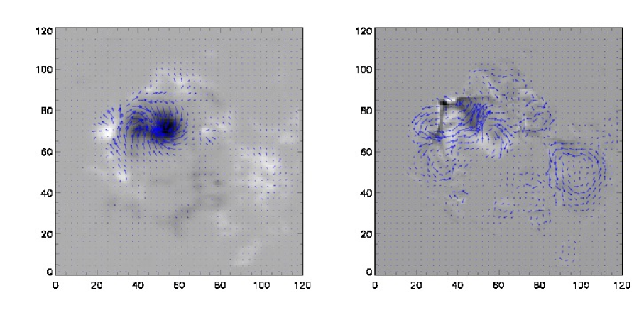
Figure 1: The left panel shows a vector magnetogram of Active Region 8210 taken with the University of Hawaii’s IVM instrument. This dataset is described in Welsch et al. (2004). Arrows show the directions and amplitudes of $B_{x}$ and $B_{y}$, and the background image shows the amplitude of $B_{z}$. The right panel shows a “vector electrogram” (a three-dimensional vector electric field map) of the active region, using the time evolution of ${\mathbf{B}}$ to estimate ${\mathbf{E}}$. Arrows show estimated directions and amplitudes of $E_{x}$ and $E_{y}$, while the background image shows the estimated amplitude of $E_{z}$. The example shown here displays ${\mathbf{E}}$ computed using the “variational” technique (§3.3). A detailed discussion of the calculation is in §4.

Most recent research on deriving electric fields in the solar atmosphere has been done by either explicitly or implicitly invoking the ideal MHD assumption, ${\mathbf{E}}=-{\mathbf{v}}/c\times{\mathbf{B}}$, and has focused on deriving two- or three-component flow fields from time sequences of magnetograms. Such techniques can be divided into two classes, which we call “tracking methods”, and “inductive methods”.

Tracking methods, such as the local correlation tracking (LCT) approach, first developed by November & Simon (1988), find a velocity vector by computing a cross-correlation function that depends on the shift between sub-images or tiles when comparing two images. The shift that maximizes the cross-correlation function (or alternatively, minimizes an error function) is then taken to be the displacement between the two sub-images; this displacement divided by the time between the images is then defined as the average local velocity. The velocity field over the entire image is built up by repeating this process for all image locations. The LCT technique suffers from two shortcomings: (1) the technique does not assume any physical conservation laws, meaning that the derived velocity field may not have a physical connection to the real flow field in the solar atmosphere; and (2) the technique is intrinsically two-dimensional, and does not account for vertical flows or evolving three-dimensional structures in the solar atmosphere. On the other hand, LCT techniques offer the advantage of being simple and robust, and are able to use non-magnetic data, such as white-light or G-band images for estimating flow fields, though the results must then be interpreted carefully. Examples of LCT techniques in current use in the solar research community include the implementation by November & Simon (1988), FLCT (Fisher & Welsch, 2008), and Lockheed-Martin’s LCT code (Title et al., 1995; Hurlburt et al., 1995).

Inductive methods of flow inversion from magnetograms were pioneered by Kusano et al. (2002), who used a combination of horizontal flow velocities derived from LCT techniques applied to the normal component of vector magnetograms, along with a solution to the vertical component of the magnetic induction equation, to derive a three-component flow field from a sequence of vector magnetograms. An alternate approach, using the same idea, but adding the interpretation of Démoulin & Berger (2003) plus a Helmholtz decomposition of the “flux transport velocity” was proposed by Welsch et al. (2004). Longcope (2004) combined the vertical component of the induction equation with a variational constraint that minimizes the total kinetic energy of the photosphere while still obeying the normal component of the induction equation. Additional techniques minimize a localized error functional while ensuring that the vertical component of the induction equation is satisfied (Schuck, 2006, 2008).

Kusano et al. (2002) observed that the $\partial B_{x}/\partial t$ and $\partial B_{y}/\partial t$ components of the induction equation involve vertical derivatives of horizontal electric field terms ($\partial E_{y}/\partial z$ and $\partial E_{x}/\partial z$, respectively). They noted that these electric field components are unconstrained by single-height vector magnetogram sequences. Consequently, while the two horizontal components of the induction equation provide more information about the evolution of the vector magnetic field, they introduce two more unknowns to the system.

The primary goal of this paper is to explore the extent to which an electric field consistent with the evolution of all three components of ${\mathbf{B}}$ can be derived from a sequence of single-height vector magnetograms, despite incomplete information about $\partial E_{x}/\partial z$ and $\partial E_{y}/\partial z$. We first show that it is possible to derive an electric field whose curl is equal to the time derivatives of all three components of ${\mathbf{B}}$. However, this electric field is not unique, and knowledge of additional physics of the electric field formation is necessary to further constrain the solution. We then show that a solution for the electric field, under the assumptions of ideal MHD, can be derived through the use of an iterative procedure, or alternatively, as the solution of a variational problem. We will compare and contrast these solutions with results from an MHD simulation, where the electric field is known. To illustrate this methodology with real data, we then apply these techniques to a set of vector magnetograms of NOAA AR8210 from 1 May 1998. Figure 1 shows a vector electric field map (a “vector electrogram”) of NOAA AR8210, along with a vector magnetogram of the same active region, derived using one of the techniques discussed in this paper.

The remainder of this paper is structured as follows. In §2, we derive solutions to the electric field given the vector magnetic field evolution in a single horizontal plane. These solutions use the poloidal-toroidal (Chandrasekhar, 1961; Moffatt, 1978) decomposition of the electric field.

In §3 we show how additional physics describing the electric field can be included by exploring two approaches, one iterative and the other variational, both aiming for the construction of an ideal MHD electric field consistent with ${\mathbf{E}}=-{\mathbf{v}}/c\times{\mathbf{B}}$. While the ideal MHD assumption is believed to be a good approximation in the photosphere, the variational formalism has been generalized to include non-ideal effects. In §3 we also compare and constrast electric fields derived with our techniques to a test case where the true solutions are known, and in §4 with an example using real vector magnetic field data. We discuss and summarize our results in §5.

2 Poloidal-Toroidal Decomposition

2.1 Decomposing the Magnetic Field and its Time Derivative

The poloidal-toroidal decomposition (henceforth PTD) of the magnetic field into two scalar potentials is well-known among dynamo theorists (Moffatt, 1978) and has been used extensively in MHD models of the solar interior that employ the anelastic approximation (Glatzmaier, 1984; Lantz & Fan, 1999; Fan et al., 1999; Brun et al., 2004). The formalism appears to have been introduced by Chandrasekhar (1961). Here, we will briefly discuss the PTD of the magnetic field, but will focus most of our effort on the PTD of the partial time derivative of the magnetic field, because of its connection to the electric field. Here we use ${\mathbf{B}}$ to refer to a snapshot of the magnetic field within the vector magnetogram field of view, and $\dot{\mathbf{B}}$ to refer to its partial time derivative.

Given a snapshot of the three-component magnetic field distribution in Cartesian coordinates, one can write ${\mathbf{B}}$ as follows:

$${\mathbf{B}}=\mbox{\boldmath$\nabla$}\times\mbox{\boldmath$\nabla$}\times{\mathcal{B}}{\mathbf{\hat{z}}}+\mbox{\boldmath$\nabla$}\times{\mathcal{J}}{\mathbf{\hat{z}}}.$$ (1)

Here, ${\mathcal{J}}$ is referred to as the “toroidal” potential, and ${\mathcal{B}}$ as the “poloidal” potential. The vector potential ${\mathbf{A}}$ is then given by

$${\mathbf{A}}=\mbox{\boldmath$\nabla$}\times{\mathcal{B}}{\mathbf{\hat{z}}}+{\mathcal{J}}{\mathbf{\hat{z}}}+\mbox{\boldmath$\nabla$}\xi,$$ (2)

where $\xi$ is a gauge potential, left unspecified.

Taking the partial time derivative of equation (1) leads to an equation of exactly the same form for $\dot{\mathbf{B}}$ in terms of the partial time derivatives $\dot{\mathcal{B}}$ and $\dot{\mathcal{J}}$:

$$\dot{\mathbf{B}}=\mbox{\boldmath$\nabla$}\times\mbox{\boldmath$\nabla$}\times\dot{\mathcal{B}}{\mathbf{\hat{z}}}+\mbox{\boldmath$\nabla$}\times\dot{\mathcal{J}}{\mathbf{\hat{z}}}\ .$$ (3)

The vector ${\mathbf{\hat{z}}}$ is assumed to point in the vertical direction, $i.e.$ normal to the photosphere. A subscript $z$ will denote vector components in the ${\mathbf{\hat{z}}}$ direction, and a subscript $h$ will denote vector components or derivatives in the locally horizontal directions, parallel to the tangent plane of the photosphere.

It is useful to rewrite equations (1) and (3) in terms of horizontal and vertical derivatives as

$${\mathbf{B}}=\mbox{\boldmath$\nabla$}_{h}\left(\partial{\mathcal{B}}\over\partial z\right)+\mbox{\boldmath$\nabla$}_{h}\times{\mathcal{J}}{\mathbf{\hat{z}}}-\nabla_{h}^{2}{\mathcal{B}}{\mathbf{\hat{z}}},$$ (4)

and

$$\dot{\mathbf{B}}=\mbox{\boldmath$\nabla$}_{h}\left(\partial\dot{\mathcal{B}}\over\partial z\right)+\mbox{\boldmath$\nabla$}_{h}\times\dot{\mathcal{J}}{\mathbf{\hat{z}}}-\nabla_{h}^{2}\dot{\mathcal{B}}{\mathbf{\hat{z}}}.$$ (5)

The PTD of $\dot{\mathbf{B}}$ has a useful connection to observation. Examining only the z-component of equation (5), one finds

$$\nabla_{h}^{2}\dot{\mathcal{B}}=-\dot{B}_{z}\ ,$$ (6)

where $\dot{B}_{z}$ is the partial time derivative of the vertical component of the magnetic field, and $\nabla_{h}^{2}$ is the horizontal contribution to the Laplacian. Thus knowledge of $\dot{B}_{z}$ in a layer yields a solution for $\dot{\mathcal{B}}$ by solving a horizontal, two-dimensional Poisson equation.

Taking the curl of equation (5) and examining only the z-component of the result, one finds

$$\nabla_{h}^{2}\dot{\mathcal{J}}=-(4\pi/c)\dot{J}_{z}=-{\mathbf{\hat{z}}}\cdot(\mbox{\boldmath$\nabla$}\times\dot{\mathbf{B}}_{h}).$$ (7)

Knowing the time derivative of the horizontal field $\dot{\mathbf{B}}_{h}$ in a layer, and hence the vertical component of its curl, determines $\dot{\mathcal{J}}$ in that layer, from solutions to another Poisson equation.

Finally, taking the horizontal divergence of equation (5) results in

$$\nabla_{h}^{2}({\partial\dot{\mathcal{B}}/\partial z})=\mbox{\boldmath$\nabla$}_{h}\cdot\dot{\mathbf{B}}_{h}.$$ (8)

Here, knowing the horizontal divergence of $\dot{\mathbf{B}}_{h}$ allows one to determine $\partial\dot{\mathcal{B}}/\partial z$, once again by solving a two-dimensional Poisson equation.

It is worth noting an additional implication of equation (8). From the solenoidal nature of ${\mathbf{B}}$ it follows that

$$\mbox{\boldmath$\nabla$}_{h}\cdot\dot{\mathbf{B}}_{h}=-\partial\dot{B}_{z}/\partial z\ .$$ (9)

Thus equation (8) can be regarded as the partial z-derivative of equation (6), yet no depth derivatives of the data were needed to evaluate it. We return to this point later.

To find the PTD of the magnetic field itself rather than its time derivative, the quantities ${\mathcal{B}}$, ${\mathcal{J}}$, and $\partial{\mathcal{B}}/\partial z$ obey exactly the same Poisson equations (6-8) above, but with all of the overdots in the equations removed. This description of ${\mathbf{B}}$ allows for an alternate computation of potential magnetic fields valid at the vector magnetogram surface (Appendix A), in which the divergence of ${\mathbf{B}}_{h}$ taken from the vector magnetogram can be incorporated into the solution. This formulation for the potential magnetic field has applications for: (i) estimating the flux of free magnetic energy, $e.g.$, equation (23) of Welsch (2006), where one needs to subtract the measured and the potential-field values of the horizontal magnetic field, and (ii) computing the vector-potential ${\mathbf{A}}_{P}$ of the potential field, useful in estimating the magnetic helicity flux. The horizontal magnetic field can be decomposed into the potential-field contribution $\mbox{\boldmath$\nabla$}_{h}(\partial{\mathcal{B}}/\partial z)$ and the non-potential contribution ${\mathbf{B}}^{{\mathcal{J}}}_{h}=\mbox{\boldmath$\nabla$}_{h}\times{\mathcal{J}}{\mathbf{\hat{z}}}$ (see Appendix A). Welsch’s flux of free energy then becomes

$$S^{\rm free}_{z}={1\over 4\pi}c{\mathbf{E}}_{h}\times{\mathbf{B}}^{{\mathcal{J}}}_{h}\ ,$$ (10)

where methods of estimating ${\mathbf{E}}$ will be discussed below.

2.2 Finding an Electric Field from Faraday’s Law

Now, compare equations (3) and (5) with Faraday’s law relating the time derivative of ${\mathbf{B}}$ to the curl of the electric field:

$$\dot{{\mathbf{B}}}=-c\mbox{\boldmath$\nabla$}\times{\mathbf{E}}$$ (11)

Equating the expressions for $\dot{{\mathbf{B}}}$, one finds this expression for $c\mbox{\boldmath$\nabla$}\times{\mathbf{E}}$:

$$c\mbox{\boldmath$\nabla$}\times{\mathbf{E}} = -\mbox{\boldmath$\nabla$}\times\mbox{\boldmath$\nabla$}\times\dot{\mathcal{B}}{\mathbf{\hat{z}}}-\mbox{\boldmath$\nabla$}\times\dot{\mathcal{J}}{\mathbf{\hat{z}}}$$ (12)

$$= -\mbox{\boldmath$\nabla$}_{h}(\partial\dot{\mathcal{B}}/\partial z)-\mbox{\boldmath$\nabla$}_{h}\times\dot{\mathcal{J}}{\mathbf{\hat{z}}}+\nabla_{h}^{2}\dot{\mathcal{B}}{\mathbf{\hat{z}}}.$$ (13)

Uncurling equation (12) yields this expression for the electric field ${\mathbf{E}}$:

$$c{\mathbf{E}}=-\mbox{\boldmath$\nabla$}\times\dot{\mathcal{B}}{\mathbf{\hat{z}}}-\dot{\mathcal{J}}{\mathbf{\hat{z}}}-c\mbox{\boldmath$\nabla$}\psi\equiv c{\mathbf{E}}^{I}-c\mbox{\boldmath$\nabla$}\psi.$$ (14)

In the process of uncurling equation (12), it is necessary to add the (three-dimensional) gradient of an unspecified scalar potential $\psi$ to the expression for the total electric field. The potential $\psi$ can be equated to $-\dot{\xi}/c+\lambda$, where $\xi$ is the gauge potential from equation (2), and $\lambda$ is some other potential function. However, we simply let the electric field potential $\psi$ absorb both contributions, and will not use the gauge $\xi$. The part of ${\mathbf{E}}$ without the contribution from $-\mbox{\boldmath$\nabla$}\psi$ will be henceforth denoted ${\mathbf{E}}^{I}$, the purely inductive contribution to the electric field.

We have derived an expression for $\mbox{\boldmath$\nabla$}\times{\mathbf{E}}$, including the two horizontal components of the induction equation, simply by using time derivative information contained within a single layer, even though those two components of the induction equation include vertical derivatives of $E_{x}$ and $E_{y}$. This was made possible by equation (8), which enabled the evaluation of the needed depth derivatives through the relation $\mbox{\boldmath$\nabla$}\cdot\dot{{\mathbf{B}}}=0$.

2.3 Boundary Conditions

To solve the three Poisson equations (6), (7), and (8), one must consider their boundary conditions. For many of the MHD simulation test cases we have used, the simulation vector fields obey periodic boundary conditions, which makes the problem straightforward: one can use Fast Fourier Transform (FFT) techniques to solve the Poisson equations without special consideration for boundary conditions (see Appendix C). For an arbitrary vector magnetogram taken over a finite area, however, the magnetic field will generally not be periodic, but will be determined by the measured fields on the boundary. For equations (7) and (8), the horizontal components of $\dot{\mathbf{B}}$ determine the boundary conditions for $\dot{\mathcal{J}}$ and $\partial\dot{\mathcal{B}}/\partial z$ from the x and y components of the primitive equation (5):

$$\dot{B}_{x}={\partial\over\partial x}{\partial\dot{\mathcal{B}}\over\partial z}+{\partial\dot{\mathcal{J}}\over\partial y},$$ (15)

and

$$\dot{B}_{y}={\partial\over\partial y}{\partial\dot{\mathcal{B}}\over\partial z}-{\partial\dot{\mathcal{J}}\over\partial x}\ .$$ (16)

From these equations, coupled Neumann boundary conditions can be derived:

$${\partial\over\partial n}{\partial\dot{\mathcal{B}}\over\partial z}=\dot{B}_{n}-{\partial\dot{\mathcal{J}}\over\partial s},$$ (17)

and

$${\partial\dot{\mathcal{J}}\over\partial n}=-\dot{B}_{s}+{\partial\over\partial s}{\partial\dot{\mathcal{B}}\over\partial z}\ ,$$ (18)

where subscript $n$ denotes components or derivatives in the direction of the outward normal from the boundary of the magnetogram, and subscript $s$ denotes components or derivatives in the counter-clockwise direction along the magnetogram boundary.

The choice of boundary conditions for $\dot{\mathcal{B}}$ in equation (6) can have subtle effects on the solution $\dot{B}_{z}$. If homogeneous Neumann boundary conditions (derivative normal to the magnetogram boundary specified with zero slope) are applied to $\dot{\mathcal{B}}$, then the horizontal curl of ${\mathbf{E}}_{h}^{I}$ around the magnetogram boundary necessarily vanishes, meaning the average value of $\dot{B}_{z}$ within the magnetogram is forced to zero. If the average value of $\dot{B}_{z}$ is nonzero, the solutions will not reflect this. This problem can be corrected post facto, however, by adding a correction term to the electric field – see Appendix E.

Applying homogenous Dirichlet boundary conditions (setting $\dot{\mathcal{B}}$ to zero at the boundaries) for the solution of equation (6) for $\dot{\mathcal{B}}$ can also result in artifacts if care is not taken. Homogenous Dirichlet boundary conditions on $\dot{\mathcal{B}}$ imply no net change in $\dot{\mathcal{B}}$ across the magnetogram, resulting in average $x-$ and $y-$ components of the electric field ${\mathbf{E}}_{h}^{I}$ that are zero. Some evolutionary patterns, such as the emergence and separation of a simple magnetic bipole oriented in the $x-$ direction should result in a non-zero average value of $E_{y}^{I}$, because the opposite polarities have opposite velocities. Thus, if Dirichlet boundary conditions are used in the solution of equation (6) for $\dot{\mathcal{B}}$, some other technique must be used to find the magnetogram-averaged values of $E_{x}^{I}$ and $E_{y}^{I}$.

The coupled boundary conditions (17-18) for the two Poisson equations (7-8) are degenerate, in that there is a family of coupled non-zero solutions to the homogeneous Cauchy-Riemann equations for $\dot{\mathcal{J}}$ and $\partial\dot{\mathcal{B}}/\partial z$:

$${\partial\over\partial x}\left({\partial\dot{\mathcal{B}}\over\partial z}\right)=-{\partial\dot{\mathcal{J}}\over\partial y},$$ (19)

and

$${\partial\over\partial y}\left({\partial\dot{\mathcal{B}}\over\partial z}\right)={\partial\dot{\mathcal{J}}\over\partial x}$$ (20)

which satisfy the boundary conditions for zero time derivative of the horizontal magnetic field on the boundary. These solutions can be added to solutions for $\dot{\mathcal{J}}$ and $\partial\dot{\mathcal{B}}/\partial z$ without changing the time derivative of the horizontal field on the boundary. Solutions to equations (19-20) also are harmonic, $i.e.$ each of the two solutions also obey the two-dimensional (horizontal) Laplace’s equation.

The boundary conditions needed to solve the Poisson equations for ${\mathcal{B}}$, ${\mathcal{J}}$, and $\partial{\mathcal{B}}/\partial z$ (if one needs to perform the PTD on ${\mathbf{B}}$, rather than $\dot{\mathbf{B}}$) are identical to the boundary conditions described above, but with all of the overdots removed. The Cauchy Riemann degeneracy described above also applies to the solutions of ${\mathcal{J}}$ and $\partial{\mathcal{B}}/\partial z$.

Even without considering $\mbox{\boldmath$\nabla$}\psi$, the degeneracy of the solutions for $\dot{\mathcal{J}}$ and $\partial\dot{\mathcal{B}}/\partial z$ for non-periodic boundary conditions means that particular solutions of the homogeneous Cauchy-Riemann equations can be added to the solutions for the inductive electric field $c{\mathbf{E}}^{I}$ without affecting $\mbox{\boldmath$\nabla$}\times{\mathbf{E}}$. This means there is some freedom to specify the solution of $\dot{\mathcal{J}}$ or $\partial\dot{\mathcal{B}}/\partial z$ at the boundary. This freedom cannot be applied to both functions simultaneously, however, since the two solutions are coupled together. In practice, this means that one could choose to set the derivatives parallel to the boundary of one of these two functions to zero, for example, while still obeying the coupled boundary conditions (17) and (18). For an illustration of this degeneracy applied to the PTD solutions for ${\mathbf{B}}$, see Figure 2.

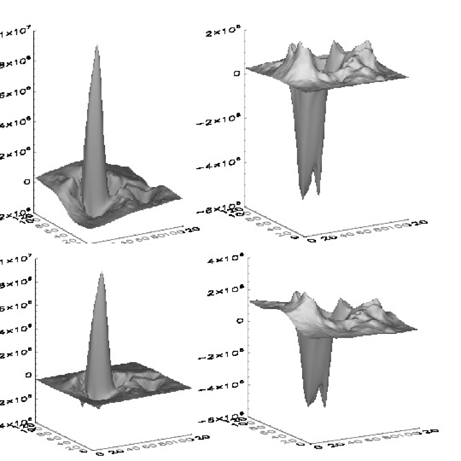
Figure 2: The top two panels show Poisson equation solutions for $\partial{\mathcal{B}}/\partial z$ (left) and ${\mathcal{J}}$ (right) within the AR 8210 magnetogram field-of-view, under the assumption that $\partial{\mathcal{J}}/\partial s=0$ along the magnetogram boundary. The AR8210 vector magnetogram data is discussed further in §4. The bottom two panels show Poisson equation solutions for the same two functions under the assumption that $\partial/\partial s(\partial{\mathcal{B}}/\partial z)=0$. The difference between the upper and lower sets of solutions obey the homogeneous Cauchy-Riemann equations. The two different sets of functions yield identical values for the horizontal components of the magnetic field.

When periodic boundary conditions cannot be assumed, equation (14) shows that the electric field on the boundary of the magnetogram determines the boundary conditions for $\dot{\mathcal{B}}$ and $\psi$:

$${\partial\dot{\mathcal{B}}\over\partial n}=cE_{s}+c{\partial\psi\over\partial s},$$ (21)

and

$$c{\partial\psi\over\partial n}=-cE_{n}-{\partial\dot{\mathcal{B}}\over\partial s}.$$ (22)

These coupled Neumann boundary conditions have a similar form as those for $\dot{\mathcal{J}}$ and $\partial\dot{\mathcal{B}}/\partial z$, (equations [17-18]) except that they depend on horizontal electric fields rather than on time derivatives of the horizontal magnetic fields. The practical difficulty with using equations (21-22) is that generally one does not know the behavior of the horizontal electric field vector on the boundaries if the boundaries are in regions of strong, evolving magnetic field . On the other hand, if one can take the boundaries along regions with weak average magnetic field strength, one could probably set $E_{n}$ and $E_{s}$ to zero along the boundaries.

3 Determining the Scalar Potential

3.1 The Implications of Not Specifying $\psi$

We can test our approach by applying equations (12) and (14) to the magnetic evolution sampled from a thin slab of an MHD simulation, in which ${\mathbf{E}}$ and $\mbox{\boldmath$\nabla$}\times{\mathbf{E}}$ are both known. How well do the derived results compare with the known electric field, and with the curl of that electric field?

To address this question, we use the results from the ANMHD simulations described in Welsch et al. (2007), which have been used for several studies of velocity field inversions (Welsch & Fisher, 2008; Schuck, 2008). This simulation models a magnetic bipole emerging through a strongly convecting layer. To compute the reconstructed distribution of $\mbox{\boldmath$\nabla$}\times{\mathbf{E}}$ and ${\mathbf{E}}$ using PTD, we use time differences from two consecutive output steps from the MHD simulation to find estimates of the time derivative of the three components of ${\mathbf{B}}$. From these three components, the three Poisson equations (6-8) can be solved, subject to boundary conditions (17-18) for $\partial\dot{\mathcal{B}}/\partial z$ and $\dot{\mathcal{J}}$. To solve the three Poisson equations along with these coupled boundary conditions, we first use a simple successive over-relaxation method to solve the equation for $\dot{\mathcal{B}}$, assuming homogenous Neumann (zero gradient) boundary conditions. We choose Neumann over Dirichlet boundary conditions because Dirichlet boundary conditions on $\dot{\mathcal{B}}$ lead to zero average horizontal electric field within the magnetogram (see earlier discussion in §2.3). To solve the two Poisson equations (7-8) along with their coupled Neumann boundary conditions (equations [17] and [18]), we have adapted the Newton-Krylov solver from RADMHD (Abbett, 2007) to solve this elliptic system simultaneously.

The top panels of Figure 3 show the curl of the electric field obtained from time differences in the magnetic field between adjacent snapshots of the magnetic field evolution. The middle panels of the Figure show the reconstructed distribution of $\mbox{\boldmath$\nabla$}\times{\mathbf{E}}$ as obtained from equation (13). The bottom panels show scatter plots between the known and reconstructed values of $\mbox{\boldmath$\nabla$}\times{\mathbf{E}}$. One can see that the reconstructed components of $\mbox{\boldmath$\nabla$}\times{\mathbf{E}}$ show good agreement with the original values from the MHD code.

If one ignores the contribution from $\mbox{\boldmath$\nabla$}\psi$ in equation (14), which is equivalent to assuming that ${\mathbf{E}}$ is equal to ${\mathbf{E}}^{I}$, it is straightforward to compare the reconstructed electric field ${\mathbf{E}}^{I}$ with that used in the ANMHD code. The top panels of Figure 4 show the actual components of the electric field used in the MHD simulation, while the middle panels show the electric field components from equation (14) approximating ${\mathbf{E}}$ by ${\mathbf{E}}^{I}$. The bottom panels show scatter plots of the reconstructed electric field components as a function of the known values.

The velocity inversion methods tested in Welsch et al. (2007) also included comparisons between the ANMHD and reconstructed electric field components computed by assuming $c{\mathbf{E}}=-{\mathbf{v}}\times{\mathbf{B}}$ (see their Figures 11 and 12). Welsch et al. (2007) showed that the simulation data for $\dot{B}_{z}$, computed by differencing two $B_{z}$ images in time, matched $-c{\mathbf{\hat{z}}}\cdot(\mbox{\boldmath$\nabla$}\times{\mathbf{E}})$, computed using simple second-order finite difference formulae to evaluate the spatial derivatives applied to the average of the electric fields at the two adjacent times. Hence, it is possible to make a direct comparison between the PTD derived electric field values reported here and those from several velocity inversion methods, including LCT techniques. The results reported in Welsch et al. (2007) include only “strong field” pixel locations where $|B_{z}|>370{\rm G}$, 5% of the maximum field strength in this simulation of subsurface magnetic evolution. Accordingly, to make a direct comparison, we compute rank-order correlation coefficients between the PTD-derived electric field components with those from ANMHD, including only the strong field locations. The rank-order correlation coefficients for the $x-$, $y-$, and $z-$ components of ${\mathbf{E}}$ are $0.76$, $0.87$, and $0.94$, respectively. This metric compares favorably with all of the techniques shown in Figures 11 and 12 of Welsch et al. (2007), showing better correlation coefficients for $E_{x}$ and $E_{y}$ than all the methods except MEF, and comparable correlation coefficients to MEF. All the methods, including PTD, show good correlation coefficients for $E_{z}$.

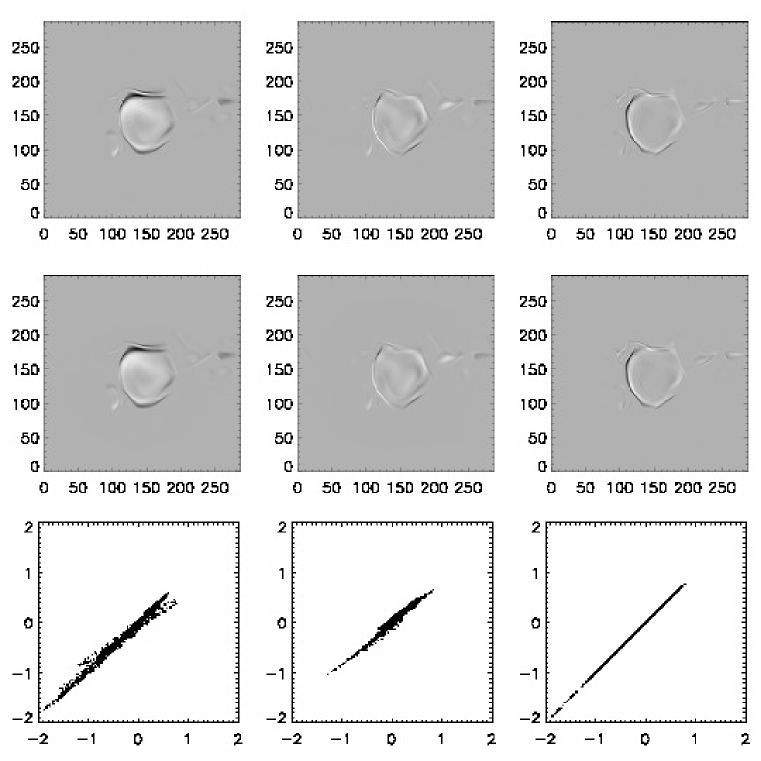
Figure 3: Top panels show the values of the $x-$, $y-$, and $z-$ components of $c\mbox{\boldmath$\nabla$}\times{\mathbf{E}}=-\partial{\mathbf{B}}/\partial t$ taken from the ANMHD simulations described in the text. The middle panels show the same components of $c\mbox{\boldmath$\nabla$}\times{\mathbf{E}}$ determined with the PTD formalism (equations [12-13]). The bottom panels show scatter-plots of the original versus derived values of the $x-$, $y-$, and $z-$ components of $c\mbox{\boldmath$\nabla$}\times{\mathbf{E}}$. Note the scatter-plots for the $x-$ and $y-$ components of $c\mbox{\boldmath$\nabla$}\times{\mathbf{E}}$ are not as tight as the $z-$ component. This stems from using finite difference operations for the Laplacian that aren’t strictly compatible with the finite difference operations we have used to evaluate the curl and divergence operators. We have also performed similar comparisons for FFT-derived solutions (Appendix C), which can be applied here, since ANMHD does assume periodic boundary conditions. In that case, the corresponding x,y scatter-plots are considerably tighter than the ones shown here. All of the grayscale images are plotted using the same scale.

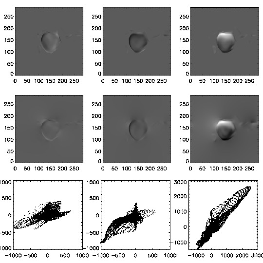
Figure 4: Top panels show the values of the $x-$, $y-$,and $z-$ components of $c{\mathbf{E}}$ taken from the ANMHD simulations described in the text. The middle panels show the same components of $c{\mathbf{E}}$ determined with the PTD formalism (equation [12]) assuming $\mbox{\boldmath$\nabla$}\psi=0$. Bottom panels show scatter plots of the $x-$,$y-$,$z-$ components of $c{\mathbf{E}}$ derived from the PTD formalism versus the ANMHD components of $c{\mathbf{E}}$. Note that compared to scatter-plots comparing $\mbox{\boldmath$\nabla$}\times{\mathbf{E}}$ between the simulation data and the PTD results, the results here show considerable scatter. All of the grayscale images are plotted using the same scale.

Despite the good performance of PTD compared to the velocity inversion methods for strong-field locations, a scatterplot comparison between the original and reconstructed electric fields is poor when all points are considered (the bottom panels of Figure 4). This contrasts with the scatterplot comparison between actual and reconstructed values of $\mbox{\boldmath$\nabla$}\times{\mathbf{E}}$ which showed good agreement.

Why is this? The problem occurs because of the under-determination of the electric field. The PTD formalism guarantees that the electric field will obey Faraday’s law, but no other information about additional physical mechanisms that would determine the electric field has been incorporated. Any additional electric field contribution that can be represented by the gradient of a scalar function is left completely unspecified. Evidently setting $\mbox{\boldmath$\nabla$}\psi=0$ in the PTD solution (equation 14) is inconsistent with the electric field as specified in the ANMHD simulation. Therefore, finding an equation that better describes $\mbox{\boldmath$\nabla$}\psi$ is essential for providing a better performance of the PTD method.

Since ${\mathbf{E}}\simeq-{\mathbf{v}}/c\times{\mathbf{B}}$ in these nearly ideal ANMHD data, ${\mathbf{E}}$ is perpendicular to ${\mathbf{B}}$. Considering only the $c{\mathbf{E}}^{I}\equiv-\mbox{\boldmath$\nabla$}\times\dot{\mathcal{B}}{\mathbf{\hat{z}}}-\dot{\mathcal{J}}{\mathbf{\hat{z}}}$ contributions from the poloidal and toroidal terms in equation (14), and decomposing the vectors into the directions parallel and perpendicular to ${\mathbf{B}}$, one finds contributions that are roughly equal in the parallel and perpendicular directions. To better reconstruct the actual electric field, it will be necessary to add a potential electric field that largely cancels out the components of ${\mathbf{E}}$ that are parallel to ${\mathbf{B}}$. The challenge is to derive an equation for $\psi$ from physical or mathematical principles that does this, while also yielding a physically reasonable solution for the resulting total electric field.

3.2 Deriving an Electric Potential I. - An Iterative Approach

Here, we describe a technique to determine a potential function that is consistent with ideal MHD (${\mathbf{E}}\cdot{\mathbf{B}}=0$), using a purely ad-hoc iterative approach. The total electric field is

$${\mathbf{E}}={\mathbf{E}}^{I}-\mbox{\boldmath$\nabla$}\psi\ ,$$ (23)

where as before, ${\mathbf{E}}^{I}$ is the inductive contribution found using the PTD formalism and $-\mbox{\boldmath$\nabla$}\psi$ is the potential contribution. We wish to define $\psi$ in such a way that the components of ${\mathbf{E}}$ parallel to ${\mathbf{B}}$ are minimized.

In step 1 of the procedure, we decompose $\mbox{\boldmath$\nabla$}\psi$ into three orthogonal directions by writing

$$\mbox{\boldmath$\nabla$}\psi=s_{1}(x,y){\mathbf{\hat{b}}}+s_{2}(x,y){\mathbf{\hat{z}}}\times{\mathbf{\hat{b}}}+s_{3}(x,y)\ {\mathbf{\hat{b}}}\times({\mathbf{\hat{z}}}\times{\mathbf{\hat{b}}})$$ (24)

Here, ${\mathbf{\hat{b}}}$ is the unit vector pointing in the direction of ${\mathbf{B}}$.

In step 2, we set $s_{1}(x,y)$ equal to ${\mathbf{E}}^{I}\cdot{\mathbf{\hat{b}}}$. This ensures that $-\mbox{\boldmath$\nabla$}\psi$ acts to cancel the component of ${\mathbf{E}}_{I}$ parallel to ${\mathbf{\hat{b}}}$. The function $s_{1}(x,y)$ will remain invariant during the rest of the iteration procedure.

In step 3, given the latest guess for $\psi$, we evaluate the functions $s_{2}(x,y)$ and $s_{3}(x,y)$ by dotting each of the vectors on the right hand side of equation (24) with equation (24), itself, yielding

$$s_{2}(x,y)={{\mathbf{\hat{z}}}\cdot({\mathbf{b}}_{h}\times\mbox{\boldmath$\nabla$}_{h}\psi)\over b_{h}^{2}}\ ,$$ (25)

and

$$s_{3}(x,y)={\partial\psi\over\partial z}-{(\mbox{\boldmath$\nabla$}_{h}\psi\cdot{\mathbf{b}}_{h})b_{z}\over b_{h}^{2}}\ .$$ (26)

Here, $b_{z}$ and $b_{h}$ represent the amplitudes of ${\mathbf{\hat{b}}}$ in the vertical and horizontal directions, respectively, and ${\mathbf{b}}_{h}$ represents only the horizontal components of ${\mathbf{\hat{b}}}$. For the initial guess during step 3, the functions $s_{2}(x,y)$ and $s_{3}(x,y)$ are set to zero.

In step 4, the horizontal divergence of $\mbox{\boldmath$\nabla$}_{h}\psi$ is taken, using the current guesses for $s_{2}(x,y)$ and $s_{3}(x,y)$. From equation (24) this results in the following two-dimensional Poisson equation for $\psi$:

$$\nabla_{h}^{2}\psi=\mbox{\boldmath$\nabla$}_{h}\cdot(s_{1}(x,y){\mathbf{b}}_{h}+s_{2}(x,y)({\mathbf{\hat{z}}}\times{\mathbf{\hat{b}}})-s_{3}(x,y)b_{z}{\mathbf{b}}_{h})$$ (27)

The values for $\psi$ are updated by solving this Poisson equation.

In step 5, the vertical gradient of $\psi$ is updated by evaluating the z-component of equation (24) employing the last guess for $s_{3}(x,y)$ (recall that $s_{1}(x,y)$ does not change between iterations):

$${\partial\psi\over\partial z}=s_{1}(x,y)b_{z}+s_{3}(x,y)b_{h}^{2}\ .$$ (28)

Step 6 consists of evaluating an error term

$$\epsilon=max{|({\mathbf{E}}_{I}-\mbox{\boldmath$\nabla$}\psi)\cdot{\mathbf{\hat{b}}}|\over|({\mathbf{E}}_{I}-\mbox{\boldmath$\nabla$}\psi)|}\ .$$ (29)

If $\epsilon$ is sufficiently small, then the iteration sequence can be terminated; otherwise steps 3-6 are repeated until the sequence converges to the desired error criterion.

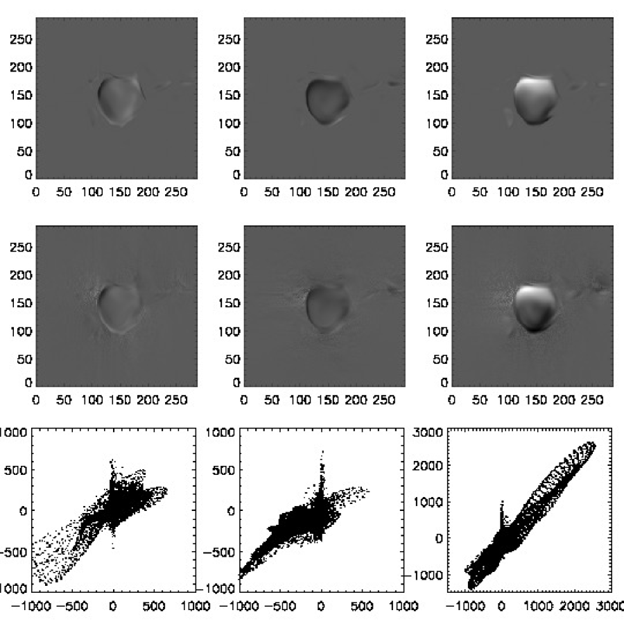
Figure 5: Top panels show the values of the $x-$, $y-$, and $z-$ components of $c{\mathbf{E}}$ taken from the ANMHD simulations described in the text. The middle panels show the same components of $c{\mathbf{E}}$ determined with the PTD formalism (equation [12]) adding $-\mbox{\boldmath$\nabla$}\psi$ as determined with the “iterative” technique of §3.2. Bottom panels show scatter plots of the $x-$, $y-$,and $z-$ components of $c{\mathbf{E}}$ derived from the PTD plus potential field solutions versus the ANMHD components of $c{\mathbf{E}}$. Note that compared to scatter-plots comparing $c{\mathbf{E}}$ from PTD solutions without the potential contribution (Figure [4]), the results here show less scatter. All of the grayscale images are plotted using the same scale.

Results of this iteration sequence applied to the PTD solutions, and compared to the true electric field results from the ANMHD simulation are shown in Figure 5. To solve the Poisson equation (27) in this example, we take advantage of the known periodic nature of the ANMHD solutions, and use FFT techniques to solve the equation for $\psi$.

From Figure 5, one can see that some of the artificial features in the PTD recovered solutions have been improved by applying the iteration scheme described here, such as the false bright halo seen in the PTD solution for $E_{x}$ on the upper left side. Further, scatterplots of $E_{x}$ and $E_{y}$ comparing results between simulation values and those with PTD only, and those with PTD plus the iteration scheme, show clear improvement by adding in the contributions from this potential function. However, the technique is by no means perfect. After applying the $\mbox{\boldmath$\nabla$}\psi$ correction derived with the iteration technique, other “shadow” artifacts, seen as faint vertical stripes below the emerging magnetic field, are visible in $e.g.$ the derived map of $E_{x}$. Computing the rank-order correlation coefficients between the ANMHD and iteration method electric fields in the strong magnetic field regions, as we did for the PTD solutions, results in values of $0.75$, $0.82$, and $0.95$ for the $x-$, $y-$ and $z-$ components of ${\mathbf{E}}$. These values are not significantly different than those for the PTD case described earlier.

In summary, this iteration scheme, or perhaps similar schemes based on related ideas, may provide a useful approach for a deriving potential electric field contribution which, when added to the PTD solutions, is consistent with ideal MHD. But we must also caution that the solutions derived via this method are not unique since the condition ${\mathbf{E}}\cdot{\mathbf{B}}=0$ does not fully constrain the potential function $\psi$. Once a solution has been obtained via this method, we can add on any additional solution $\psi^{\prime}$ which obeys the constraint $\mbox{\boldmath$\nabla$}\psi^{\prime}\cdot{\mathbf{B}}=0$, without affecting the induction equation or the condition ${\mathbf{E}}\cdot{\mathbf{B}}=0$.

It is also not clear whether this iteration technique will converge for all cases, or whether the derived solutions are mathematically well posed apart from the uniqueness issue already raised. Clearly this area needs further study.

3.3 Deriving an Electric Potential II. - A Variational Approach

The dynamics of the solar plasma is determined by the largest forces, which in regions of strong magnetic fields will involve Lorentz forces, acting in conjunction with gravity, pressure gradients, and inertial terms. To the extent that the electric field is dominated by the ideal $-{\mathbf{v}}/c\times{\mathbf{B}}$ term, then it is necessary to know the forces acting to determine the velocity field in the photosphere to determine the full electric field and thus completely specify $\psi$.

In §3.1, we demonstrated that vector magnetograms alone contain only partial information about the plasma dynamics – there simply isn’t enough information in the magnetic field data alone to uniquely specify ${\mathbf{v}}$ or ${\mathbf{E}}$. Additional information must be obtained either from other measurements or by using some other constraint.

One approach for deriving a constraint equation for $\psi$ is to use a variational principle. For example, one could adjust $\psi$ such that the electromagnetic field energy density, $(E^{2}+B^{2})/(8\pi)$, integrated over the magnetogram, is minimized. Since ${\mathbf{B}}$ itself has already been determined by the measurements, this is tantamount to finding $\psi$ such that the area integral of $E^{2}$ is minimized. The motivation for this approach is to reduce or eliminate the unphysical electric field “halos” seen in regions of negligible magnetic fields strength in Figure 4. An alternative equation for $\psi$ can be derived by minimizing $|c{\mathbf{E}}\times{\mathbf{B}}/B^{2}|^{2}$ integrated over the magnetogram, which is equivalent to minimizing the kinetic energy of flows in the photosphere, if one assumes ${\mathbf{E}}=-{\mathbf{v}}/c\times{\mathbf{B}}$. This is essentially the approach used by Longcope (2004) in his MEF technique for deriving flows from magnetograms using only the vertical component of the induction equation.

Here we derive an equation for $\psi$ which is sufficiently general that both of these cases can be included using the same formalism. We minimize the functional

$$L=\int\,dx\,dy\,W^{2}(x,y)[(E^{I}_{x}-\partial\psi/\partial x)^{2}+(E^{I}_{y}-\partial\psi/\partial y)^{2}+(E^{I}_{z}-\partial\psi/\partial z)^{2}]~{},$$ (30)

where $W^{2}(x,y)$ is an arbitrary weighting function, and $E_{x}^{I}$, $E_{y}^{I}$, and $E_{z}^{I}$ are the three components of ${\mathbf{E}}^{I}$ as it defined in equation (14).

In the photosphere, we believe the electric field ${\mathbf{E}}^{I}-\mbox{\boldmath$\nabla$}\psi$ is dominated by the ideal term $-{\mathbf{v}}/c\times{\mathbf{B}}$, but with a possible additional contribution ${\mathbf{R}}$, which can represent resistive or any other non-ideal electric field terms. We assume that ${\mathbf{R}}$ is either a known function, is determined by observation, or is specified by the user as an Ansatz. Then

$${\mathbf{E}}=-{{\mathbf{v}}\over c}\times{\mathbf{B}}+{\mathbf{R}}={\mathbf{E}}^{I}-\mbox{\boldmath$\nabla$}\psi\ .$$ (31)

By dotting ${\mathbf{E}}^{I}-\mbox{\boldmath$\nabla$}\psi$ with ${\mathbf{B}}$, one finds

$$({\mathbf{E}}^{I}-\mbox{\boldmath$\nabla$}\psi)\cdot{\mathbf{B}}={\mathbf{R}}\cdot{\mathbf{B}}.$$ (32)

This equation provides an additional constraint on the potential $\psi$, allowing us to eliminate $\partial\psi/\partial z$ in favor of $\mbox{\boldmath$\nabla$}_{h}\psi$:

$$B_{z}{\partial\psi\over\partial z}={\bf B}\cdot{\mathbf{E}}^{I}-{\bf B}_{h}\cdot{\mbox{\boldmath$\nabla$}}_{h}\psi-{\mathbf{R}}\cdot{\mathbf{B}}.$$ (33)

Note that the functional minimized in equation (30) depends on $\psi$ through its dependence on the total electric field ${\mathbf{E}}^{I}-\mbox{\boldmath$\nabla$}\psi$. In particular, the z-component of ${\mathbf{E}}$ that appears in equation (30) depends on $E_{z}^{I}-\partial\psi/\partial z$. But from the above constraint equation (33) we can see that

$$B_{z}(E_{z}^{I}-{\partial\psi\over\partial z})={\mathbf{R}}\cdot{\mathbf{B}}-{\bf B}_{h}\cdot({\mathbf{E}}_{h}^{I}-\mbox{\boldmath$\nabla$}_{h}\psi),$$ (34)

showing that $E_{z}^{I}=-\dot{\mathcal{J}}$ cancels out of the variational equation. This result shows that a solution of the variational problem for ${\mathbf{E}}^{I}-\mbox{\boldmath$\nabla$}\psi$ will be independent of the solutions for $\dot{\mathcal{J}}$ and $\partial\dot{\mathcal{B}}/\partial z$ as determined from equations (7-8) and boundary conditions (17-18). Thus the fact that $\partial\dot{\mathcal{B}}/\partial z$ and $\dot{\mathcal{J}}$ do not have unique solutions does not affect the uniqueness of the solutions for the electric field itself: In this approach, changes in $\dot{\mathcal{J}}$ are compensated by changes in $\partial\psi/\partial z$ such that $E_{z}$ is unchanged.

Performing the Euler-Lagrange minimization of equation (30) results in a second-order, two-dimensional elliptic partial differential equation for $\psi$,

$$0=\mbox{\boldmath$\nabla$}_{h}\cdot\left\{W^{2}(x,y)\left(({\mathbf{E}}^{I}_{h}-\mbox{\boldmath$\nabla$}_{h}\psi)+{\bf B}_{h}\frac{\left[{\bf B}_{h}\cdot({\mathbf{E}}^{I}_{h}-\mbox{\boldmath$\nabla$}_{h}\psi)-{\mathbf{R}}\cdot{\mathbf{B}}\right]}{B_{z}^{2}}\right)\right\}$$ (35)

Equation (35) involves a combination of both the inductive electric field from equation (14) and the potential contribution from $-\mbox{\boldmath$\nabla$}_{h}\psi$, assuming that ${\mathbf{E}}^{I}$ is given. Solving this equation for $\psi$ given ${\mathbf{E}}_{h}^{I}$ is essentially the approach taken by Longcope (2004) in the development of MEF.

Alternatively, equation (35) can be viewed as a single equation for the sum of both the inductive and potential contributions, to be determined simultaneously. If the equation for the total field can be solved, then the potential term can be found afterward by subtracting the PTD solution (equation [14]) from the solution for the total electric field.

Writing the total electric field ${\mathbf{E}}$ as ${\mathbf{E}}^{I}-\mbox{\boldmath$\nabla$}\psi$, or $E_{z}=E_{z}^{I}-\partial\psi/\partial z$, and ${\mathbf{E}}_{h}={\mathbf{E}}_{h}^{I}-\mbox{\boldmath$\nabla$}_{h}\psi$, and noting that equation (34) relates $E_{z}$ to ${\mathbf{E}}_{h}$, equation (35) can be re-written as

$$\mbox{\boldmath$\nabla$}_{h}\cdot(W^{2}/B_{z})\left({\mathbf{E}}_{h}B_{z}-E_{z}{\mathbf{B}}_{h}\right) =$$

$$-\mbox{\boldmath$\nabla$}_{h}\cdot(W^{2}/B_{z})\left({\mathbf{E}}\times{\mathbf{B}}\right)\times{\mathbf{\hat{z}}} =$$

$$-{\mathbf{\hat{z}}}\cdot\mbox{\boldmath$\nabla$}_{h}\times(W^{2}/B_{z})\left({\mathbf{E}}\times{\mathbf{B}}\right)_{h} = 0.$$ (36)

The variational approach thus leads to a local condition on the quantity $(W^{2}/B_{z})({\mathbf{E}}\times{\mathbf{B}})_{h}$, namely that it is curl-free, and thus can be represented as the gradient of a two-dimensional scalar function. Therefore, we write

$$(W^{2}/B_{z})(c{\mathbf{E}}\times{\mathbf{B}})_{h}=-\mbox{\boldmath$\nabla$}_{h}\chi.$$ (37)

We wish to derive an equation for $\chi$, starting from equation (37) and involving only known quantities from the vector magnetic field or its time derivatives. The details of the derivation are shown in Appendix G. The result is

$${-\partial B_{z}\over\partial t}+\mbox{\boldmath$\nabla$}_{h}\cdot\left({c{\mathbf{R}}\cdot{\mathbf{B}}\over B^{2}}\ {\mathbf{\hat{z}}}\times{\mathbf{B}}_{h}\right)+\mbox{\boldmath$\nabla$}_{h}\cdot\left({1\over W^{2}B^{2}}({\mathbf{B}}_{h}\cdot\mbox{\boldmath$\nabla$}_{h}\chi){\mathbf{B}}_{h}\right)=-\mbox{\boldmath$\nabla$}_{h}\cdot\left({B_{z}^{2}\over W^{2}B^{2}}\mbox{\boldmath$\nabla$}_{h}\chi\right).$$ (38)

Eventually, we will assume ${\mathbf{R}}=0$, but for now we retain it in our formalism so that non-ideal effects can be included.

If one either knows ${\mathbf{R}}$ or sets ${\mathbf{R}}\cdot{\mathbf{B}}$ to $0$, equation (38) is a two-dimensional linear elliptic partial differential equation for $\chi$, with coefficients that depend on the magnetic field components or its time derivatives. Thus we can regard the solution for $\chi$ as well-defined.

In Appendix G we determined how to find $E_{z}$ from $\chi$ via equation (G3). To find ${\mathbf{E}}_{h}$, one can take the cross-product of ${\mathbf{\hat{z}}}$ with equation (G2) and use equation (G3) to find

$$c{\mathbf{E}}_{h}=c{{\mathbf{R}}\cdot{\mathbf{B}}\over B^{2}}{\mathbf{B}}_{h}-{B_{z}^{2}\over W^{2}B^{2}}\ {\mathbf{\hat{z}}}\times\mbox{\boldmath$\nabla$}_{h}\chi-{1\over W^{2}B^{2}}\ ({\mathbf{B}}_{h}\cdot\mbox{\boldmath$\nabla$}_{h}\chi)\ {\mathbf{\hat{z}}}\times{\mathbf{B}}_{h}.$$ (39)

The Poynting flux ${\mathbf{S}}\equiv(c/(4\pi))\ {\mathbf{E}}\times{\mathbf{B}}$ has components that point along the gradient of $\chi$ in the horizontal direction as the definition (37) shows. However, we can determine the Poynting flux in the vertical direction as well by noting that ${\mathbf{S}}\cdot{\mathbf{B}}=0$, or $B_{z}S_{z}=-{\mathbf{B}}_{h}\cdot{\mathbf{S}}_{h}$. Thus we find

$${\mathbf{S}}_{h}=-{B_{z}\over 4\pi W^{2}}\mbox{\boldmath$\nabla$}_{h}\chi,$$ (40)

and

$$S_{z}={\mbox{\boldmath$\nabla$}_{h}\chi\cdot{\mathbf{B}}_{h}\over 4\pi W^{2}}.$$ (41)

Assuming that the non-ideal electric field term ${\mathbf{R}}$ is zero or negligible compared to the ideal contribution, equation (38) is greatly simplified for the two special cases of $W^{2}=1/B^{2}$ (minimum kinetic energy) and $W^{2}=1$ (minimum electric field energy). In those cases, equation (38) becomes

$$(W^{2}B^{2}=1:)\ \ \ {-\partial B_{z}\over\partial t}+\mbox{\boldmath$\nabla$}_{h}\cdot\left(({\mathbf{B}}_{h}\cdot\mbox{\boldmath$\nabla$}_{h}\chi){\mathbf{B}}_{h}\right)=-\mbox{\boldmath$\nabla$}_{h}\cdot\left(B_{z}^{2}\mbox{\boldmath$\nabla$}_{h}\chi\right).$$ (42)

and

$$(W^{2}=1:)\ \ \ \ {-\partial B_{z}\over\partial t}+\mbox{\boldmath$\nabla$}_{h}\cdot\left(({\mathbf{b}}_{h}\cdot\mbox{\boldmath$\nabla$}_{h}\chi){\mathbf{b}}_{h}\right)=-\mbox{\boldmath$\nabla$}_{h}\cdot\left(b_{z}^{2}\mbox{\boldmath$\nabla$}_{h}\chi\right).$$ (43)

In equation (43) $b_{z}$ and ${\mathbf{b}}_{h}$ represent, respectively, the vertical and horizontal components of the unit vector ${\mathbf{\hat{b}}}$ pointing in the direction of the magnetic field.

Once the variational equation for $\chi$ has been solved, how does one relate the total electric field to the PTD solutions and the potential field contribution? Since the total electric field ${\mathbf{E}}={\mathbf{E}}^{I}-\mbox{\boldmath$\nabla$}\psi$, we can subtract the ${\mathbf{E}}^{I}$ contribution of equation (14) from equations (39) and (G3) to derive these expressions for the electric field from $\mbox{\boldmath$\nabla$}\psi$:

$$-c\mbox{\boldmath$\nabla$}_{h}\psi=c{{\mathbf{R}}\cdot{\mathbf{B}}\over B^{2}}{\mathbf{B}}_{h}-{B_{z}^{2}\over W^{2}B^{2}}\ {\mathbf{\hat{z}}}\times\mbox{\boldmath$\nabla$}_{h}\chi-{1\over W^{2}B^{2}}\ ({\mathbf{B}}_{h}\cdot\mbox{\boldmath$\nabla$}_{h}\chi)\ {\mathbf{\hat{z}}}\times{\mathbf{B}}_{h}+\mbox{\boldmath$\nabla$}_{h}\times\dot{\mathcal{B}}{\mathbf{\hat{z}}}$$ (44)

and

$$-c{\partial\psi\over\partial z}=B_{z}{c{\mathbf{R}}\cdot{\mathbf{B}}\over B^{2}}-{B_{z}\mbox{\boldmath$\nabla$}_{h}\chi\cdot({{\mathbf{\hat{z}}}\times{\mathbf{B}}_{h}})\over W^{2}B^{2}}+\dot{\mathcal{J}}.$$ (45)

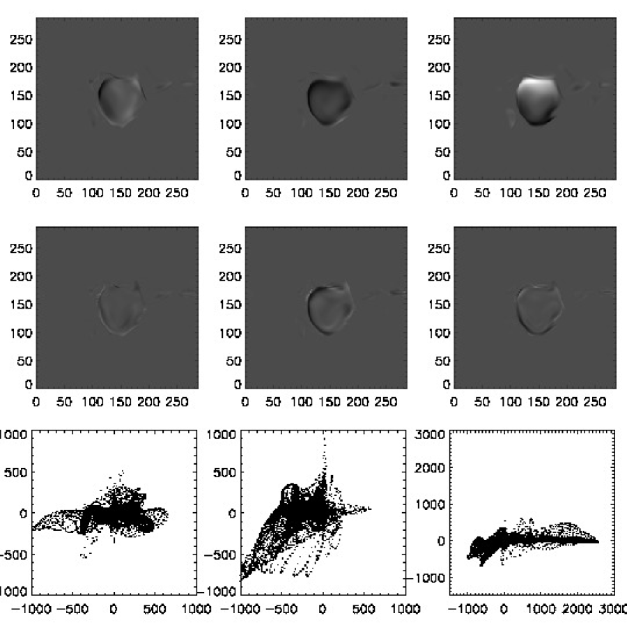
Figure 6: Top panels show the values of the $x-$, $y-$, and $z-$ components of $c{\mathbf{E}}$ taken from the ANMHD simulations described in the text. The middle panels show the same components of ${\mathbf{E}}$ determined with the variational formalism (equation [43], plus equations [G3] and [39], $i.e.$ minimizing $E^{2}$). The bottom panels show scatter-plots of the original versus derived values of the $x-$, $y-$, and $z-$ components of $c{\mathbf{E}}$. All of the grayscale images are plotted using the same scale.

The variational equation for $\chi$ incorporates the vertical component of the induction equation (the part that depends on ${\partial B_{z}}/{\partial t}$), but does not depend at all on ${\partial{\mathbf{B}}_{h}}/{\partial t}$. This means, for the variational solutions, that any observed time behavior for ${\mathbf{B}}_{h}$ can be specified independently of the time behavior for $B_{z}$.

To illustrate the variational technique, we minimize $E^{2}$ integrated over the magnetogram, ($W^{2}=1$) again using the ANMHD simulation described in §3.1. The “observed” map of $\partial B_{z}/\partial t$ is used as input, and we solved equation (43) for $\chi$, using Neumann boundary conditions (assuming zero horizontal Poynting flux entering at the horizontal boundaries). This is a very good approximation for all but a few short segments of this synthetic magnetogram boundary. Since equation (43) shows that $\chi=0$ is a solution in regions of insignificant $\dot{B}_{z}$, corresponding to the low field strength regions of the domain, the solution for $\chi$ is set to zero for magnetic fields strengths below a threshold value. Once a solution for $\chi$ is found, we verified that the horizontal components of ${\mathbf{E}}$ found from equation (39) obeyed the induction equation, $i.e.$, $c\mbox{\boldmath$\nabla$}_{h}\times{\mathbf{E}}_{h}=-\partial B_{z}/\partial t$. The resulting three components of ${\mathbf{E}}$ are shown as the middle panels in Figure 6.

The results show a generally poor agreement with ${\mathbf{E}}$ from the ANMHD simulation. Thus, at least in this case, the variational approach of minimizing $E^{2}$ does not do a good job of reproducing the actual electric field. The PTD solution by itself ($i.e.$ assuming that ${\mathbf{E}}={\mathbf{E}}^{I}$) shows better agreement with the simulation data, even though it produces spurious components of ${\mathbf{E}}$ parallel to ${\mathbf{B}}$ (which the ANMHD simulations did not have). Computing the rank-order correlation coefficients between the ANMHD and variational electric fields in the strong magnetic field regions results in values of $0.33$, $0.50$, and $0.50$ for the $x-$, $y-$, and $z-$ components of ${\mathbf{E}}$, also indicating a poor agreement with the ANMHD electric field results.

In spite of the poor comparison with the ANMHD results, the variational method did what it was designed to do: find an electric field that obeyed the induction equation, yet do this with minimum amplitude. The “halos” shown in the PTD solutions of Figure 4, for example, have been eliminated. Although the resulting electric field was not consistent with the simulation data, the variational method does yield a physically reasonable result, and stays zero in regions where one expects to find ${\mathbf{E}}$ near zero. These results motivate future exploration of other choices for $W^{2}$, to determine whether other choices result in better fits of the variational results to the MHD simulation data.

4 An Example: NOAA AR 8210

To illustrate the ideas described in the previous sections with an example using a real sequence of vector magnetograms, we apply these techniques to a pair of vector magnetograms of NOAA Active Region 8210 taken with the University of Hawaii’s Imaging Vector Magnetograph instrument (IVM) at Mees Solar Observatory on Haleakala (Mickey et al., 1996). These observations have already been described in detail in Welsch et al. (2004). We chose this observational test case because the data is well known, and we can therefore forego a detailed discussion of the data and its analysis.

The pair of vector magnetograms, separated by a period of roughly 4 hours, were first cross-correlated and shifted to remove a mean shift due to solar rotation, and then averaged to define a mean vector magnetic field, and differenced to approximate a partial time derivative of each magnetic field component.

We first apply the PTD formalism for the average vector magnetic field to derive the three fields ${\mathcal{B}}$, $\partial{\mathcal{B}}/\partial z$, and ${\mathcal{J}}$. In §2.3 we pointed out that the solutions are degenerate, in that solutions to the homogeneous Cauchy-Riemann equations can be added to the solutions for $\partial{\mathcal{B}}/\partial z$ and ${\mathcal{J}}$ without affecting the derived values of ${\mathbf{B}}_{h}$. The degeneracy can be removed by choosing to set either $\partial{\mathcal{J}}/\partial s\ =0$, or $\partial/\partial s\ (\partial{\mathcal{B}}/\partial z)=0$ (but not both) when applying boundary conditions (17) and (18) to the solutions of the Poisson equations for these two functions. We show in Figure 2 how the functions $\partial{\mathcal{B}}/\partial z$ and ${\mathcal{J}}$ differ depending on which parallel derivative is set to zero along the magnetogram boundary. Neither choice affects the derived values of ${\mathbf{B}}_{h}$, but there is a slight advantage to choosing to set $\partial{\mathcal{J}}/\partial s=0$: in that case, the observed values of $B_{n}$ are due entirely to $\partial/\partial n(\partial{\mathcal{B}}/\partial z)$, and therefore correspond to the potential-field solution that matches $B_{n}$ at the boundaries (Appendix A). That means that any contribution to the horizontal magnetic field from currents can be attributed entirely to the contribution from ${\mathcal{J}}$.

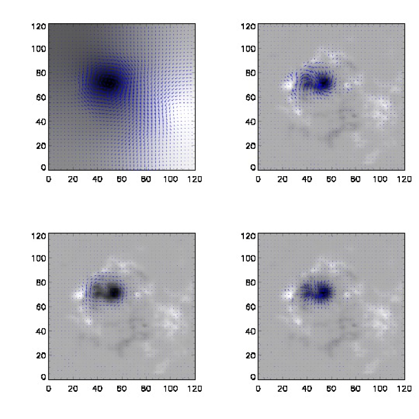
Figure 7: The upper left panel shows ${\mathcal{B}}$ as the background image, while ${\mathbf{A}}_{P}=\mbox{\boldmath$\nabla$}_{h}\times{\mathcal{B}}{\mathbf{\hat{z}}}$, the vector potential for the potential magnetic field with the same $B_{z}$ as the vector magnetogram, is shown as the arrows. The arrows in the upper right panel show ${\mathbf{B}}_{h}$, which can be decomposed into the two contributions shown in the lower two panels. The lower left panel, also with $B_{z}$ as the background image, shows the contribution to $B_{h}$ solely from $\mbox{\boldmath$\nabla$}_{h}\times{\mathcal{J}}{\mathbf{\hat{z}}}$, which shows the contributions from non-zero values of $J_{z}$. The lower right panel shows the vertical magnetic field $B_{z}$ as the background image, and the horizontal components of the potential magnetic field ${\mathbf{B}}_{h}^{P}=\mbox{\boldmath$\nabla$}_{h}\partial{\mathcal{B}}/\partial z$ (equation [A4]) as the arrows. All of the horizontal magnetic field vectors are drawn at the same scale.

These points are illustrated in Figure 7, which shows the spatial distribution of ${\mathcal{B}}$, ${\mathbf{A}}_{P}=\mbox{\boldmath$\nabla$}_{h}\times{\mathcal{B}}{\mathbf{\hat{z}}}$, $B_{z}$, ${\mathbf{B}}_{h}$, and the contributions of both the potential-field and current sources to ${\mathbf{B}}_{h}$. To remove the Cauchy-Riemann degeneracy, it was assumed that $\partial{\mathcal{J}}/\partial s=0$ along the magnetogram boundary, coinciding with the choice of the top two panels of Figure 2. A homogeneous Neumann boundary condition is used to compute ${\mathcal{B}}$: $\partial{\mathcal{B}}/\partial n=0$ along the magnetogram boundaries.

Considering next the time evolution of the magnetic field, we first apply the PTD solution to the measured values $\partial{\mathbf{B}}/\partial t$. To solve equation (6) for $\dot{\mathcal{B}}$, we have to assume a boundary condition for ${\mathbf{E}}$ at the edges of the magnetogram. Generally, this is not known, but if one is sufficiently lucky to have the magnetogram boundary located entirely in a region with zero or small magnetic fields, it is reasonable to assume that ${\mathbf{E}}=0$ along the magnetogram boundary. If one is solving only the equation for $\dot{\mathcal{B}}$ (and not solving for $\psi$ simultaneously), one can only require that one component of ${\mathbf{E}}_{h}$ vanish along the boundary. We believe it is more physical to set the component of ${\mathbf{E}}_{h}$ parallel to the boundary ($E_{s}$) to zero at the boundary, which means setting the normal derivative of $\dot{\mathcal{B}}$ to zero there (homogenous Neumann boundary conditions), motivated by the discussion in §2.3.

Our data for AR8210 includes some regions that have significant magnetic field changes along short sections of the magnetogram boundary. Since we are merely trying to demonstrate how to use these techniques with real data, our approach here is to set $\partial{\mathbf{B}}/\partial t=0$ in a narrow strip of three zones just inside the magnetogram boundary, and assume we can then set the parallel component of ${\mathbf{E}}_{h}$ ($E_{s}$) in this slightly altered test case to zero. This boundary condition is equivalent to having a zero derivative of $\dot{\mathcal{B}}$ in the direction normal to the boundary (Neumann boundary conditions). Once this assumption is made, it is also advisable to use the same Neumann boundary conditions for ${\mathcal{B}}$, so that the time evolution of ${\mathbf{A}}$ and ${\mathbf{A}}_{P}$ are consistent with ${\mathbf{E}}$ computed at the boundaries.

If one is using only the PTD solutions, it is probably also a good idea to set a physically reasonable boundary condition for $\dot{\mathcal{J}}$ at the edge of the magnetogram. For reasons similar to those described above, it seems reasonable to assume that $E_{z}=0$ along magnetogram boundaries that lie in regions of weak average field. Since $cE_{z}=-\dot{\mathcal{J}}$ in the PTD formalism, this can be achieved by choosing to set $\partial\dot{\mathcal{J}}/\partial s\ =0$ when applying the boundary conditions (17-18) to solving the Poisson equations (6-8). Making this assumption removes the Cauchy-Riemann degeneracy for the $\dot{\mathcal{J}}$ and $\partial{\dot{\mathcal{B}}}/\partial z$ solutions. This has the added consequence of allowing one to interpret the contributions of $\partial{\dot{\mathcal{B}}}/\partial z$ to $\partial{\mathbf{B}}_{h}/\partial t$ as being changes to the potential-field part of the solution.

Figure 8 shows the resulting PTD solutions for ${\mathbf{E}}^{I}$, and for $\mbox{\boldmath$\nabla$}\times{\mathbf{E}}^{I}$. Also shown are the decompositions of the curl into the evolution of the potential-field, and those driven by the observed evolution in $J_{z}$.

We have also tested the iteration technique and the variational technique on the AR 8210 vector magnetogram data. Figure 9 shows a comparison of ${\mathbf{E}}$ computed using the three different techniques. The two left panels show ${\mathbf{E}}_{h}$ and $E_{z}$ from the PTD solution, with the boundary conditions as described above. The two middle panels show the same quantities from the iterative technique, and the two right panels show the solution from the variational method.

There are common patterns in ${\mathbf{E}}_{h}$ seen in all three solutions, namely that ${\mathbf{E}}_{h}$ swirls around a region of decreasing positive $B_{z}$ on the right hand side of the magnetogram about 40% of the way up from the bottom, and all three show a common pattern near the large sunspot. But the PTD solution also shows clear evidence of artifacts as well, such as a strong horizontal electric field normal to the magnetogram boundary near the left edge that is non-existent in the variational solution, and much less pronounced in the iteration solution. The iterative technique shows that some of the artifacts in the PTD solutions are reduced, but also shows large amplitude signals in some of the weak field regions. The variational solution shows small electric field vectors in regions of small magnetic field strength, which seems physical, at least superficially. There is little resemblance between the $E_{z}$ solution found with PTD, and the $E_{z}$ maps of the iterative and variational methods. Most likely, this is because the latter two methods enforce ${\mathbf{E}}\cdot{\mathbf{B}}=0$, meaning that $E_{z}$ must be adjusted during solution algorithm such that this condition is satisfied. The iterative and variational solutions for $E_{z}$ are poorly constrained near polarity inversion lines, judging by the large fluctuations near them, probably also a consequence of forcing ${\mathbf{E}}\cdot{\mathbf{B}}=0$. This might indicate that evolution is not consistent with ideal MHD along polarity inversion lines.

Finally, we show the Poynting fluxes found from all three electric field techniques in Figure 10. In contrast to the electric fields themselves, the Poynting flux distributions are all fairly similar, showing a northward (positive in the ${\mathbf{\hat{y}}}$ direction) flux of magnetic energy out of the negative polarity sunspot, and positive vertical Poynting flux in the region south of the negative sunspot.

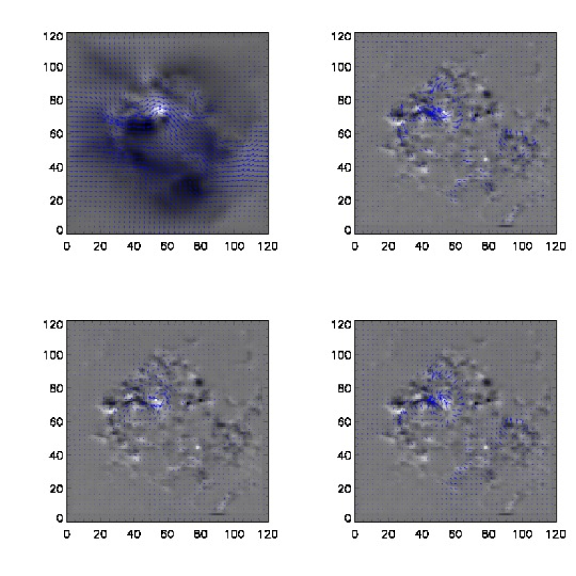
Figure 8: The upper left panel shows $cE_{z}^{I}=-\dot{\mathcal{J}}$ as the background image, while $c{\mathbf{E}}_{h}^{I}=-\mbox{\boldmath$\nabla$}_{h}\times\dot{\mathcal{B}}{\mathbf{\hat{z}}}$, the horizontal electric field vector responsible for the time evolution of $B_{z}$ from the vector magnetogram difference, is shown as the arrows. The arrows in the upper right panel show $\partial{\mathbf{B}}_{h}/\partial t$, with $\partial B_{z}/\partial t$ as the background image. The lower left panel, also with $\partial B_{z}/\partial t$ as the background image, shows the contribution to $\partial{\mathbf{B}}_{h}/\partial t$ solely from $-\mbox{\boldmath$\nabla$}_{h}\times\dot{\mathcal{J}}{\mathbf{\hat{z}}}$, which shows the contributions from non-zero values of $\partial J_{z}/\partial t$. The lower right panel shows $\partial B_{z}/\partial t$ as the background image, and the time evolution of the horizontal components of the potential magnetic field, $\partial{\mathbf{B}}_{h}^{P}/\partial t=-\mbox{\boldmath$\nabla$}_{h}\partial\dot{\mathcal{B}}/\partial z$ as the arrows. The vectors in the three panels showing changes to ${\mathbf{B}}_{h}$ are all drawn at the same scale.

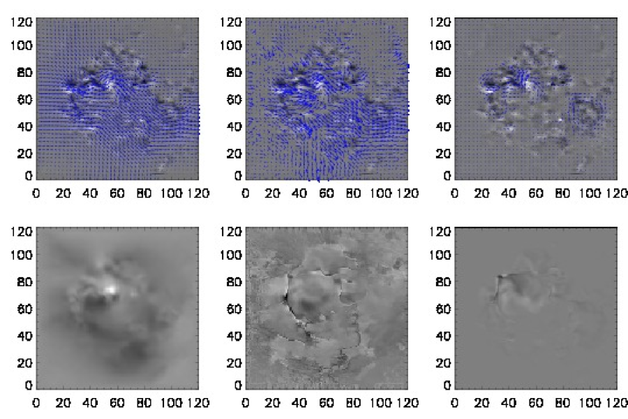
Figure 9: The top three panels show the derived horizontal electric field using the three different techniques discussed in this paper, applied to the AR 8210 vector magnetogram sequence. The background image in all three cases is $\partial B_{z}/\partial t$. The arrows in the upper left panel show values of ${\mathbf{E}}_{h}^{I}$ from the PTD algorithm with $-\mbox{\boldmath$\nabla$}\psi$ set to zero. The top middle panel shows ${\mathbf{E}}_{h}={\mathbf{E}}_{h}^{I}-\mbox{\boldmath$\nabla$}_{h}\psi$, with $\psi$ computed using the iteration technique. The top right panel shows ${\mathbf{E}}_{h}$ computed with the variational technique (minimizing $E^{2}$). The bottom three panels show $E_{z}^{I}$ (left), $E_{z}^{I}-\partial\psi/\partial z$ computed with the iteration technique (middle), and $E_{z}$ from the variational method (right). Note that $E_{z}$ is poorly behaved in the latter two cases along magnetic neutral lines. All of the electric field vectors are drawn at the same scale, and the $E_{z}$ images are displayed with the same linear grayscale colormap.

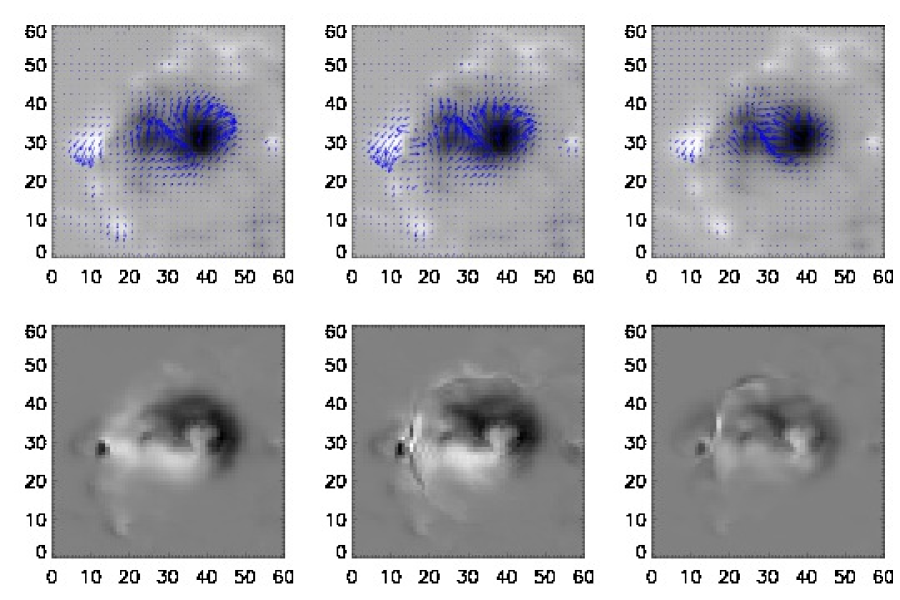
Figure 10: The top three panels show the derived horizontal Poynting flux using the different techniques discussed in this paper, applied to the AR 8210 vector magnetogram sequence. The background image in all three cases is $B_{z}$. The arrows in the upper left panel show values of ${\mathbf{S}}_{h}^{I}$ from the PTD algorithm with $-\mbox{\boldmath$\nabla$}\psi$ contribution set to zero. The top middle panel shows ${\mathbf{S}}_{h}$ computed from ${\mathbf{E}}^{I}_{h}-\mbox{\boldmath$\nabla$}\psi$ using the iteration technique. The top right panel shows ${\mathbf{S}}_{h}$ computed with the variational technique (minimizing $E^{2}$). The bottom three panels show $S_{z}^{I}$ (left), $S_{z}$ computed with the iteration technique (middle), and $S_{z}$ from the variational method (right). The vectors in the top three panels, and the grayscale images in the bottom three panels are all plotted with the same scale. For a better view of the Poynting flux structure, only a 60x60 pixel region of the vector magnetogram field of view is shown.

5 Summary and Discussion

In this paper, we introduce and demonstrate three new techniques for determining electric field distributions given a sequence of vector magnetogram observations. The following is a summary of the most important points.

The first technique, based on a poloidal-toroidal decomposition (PTD) of the time derivative of ${\mathbf{B}}$ and hence $c\mbox{\boldmath$\nabla$}\times{\mathbf{E}}$, results in a solution for ${\mathbf{E}}$ that satisfies all three components of Faraday’s law, but does not constrain any components of ${\mathbf{E}}$ derived from the gradient of a potential $\psi$. We showed in §3.1 and in §4 that the unmodified PTD solutions (assuming $\mbox{\boldmath$\nabla$}\psi=0$) result in several artifacts and non-physical effects, and argued that more physically realistic solutions for ${\mathbf{E}}$ must include contributions to the electric field from a potential function, $-\mbox{\boldmath$\nabla$}\psi$. One concern in particular is that the PTD solution has significant components of ${\mathbf{E}}$ parallel to ${\mathbf{B}}$, contradicting the ideal MHD assumption that many regard as most likely to represent the solar photosphere, and certainly contradicting the ANMHD simulation test case discussed in detail throughout §3. In spite of these defects, the electric fields found from the PTD solutions were more accurate in the strong magnetic field regions of the ANMHD simulation than those determined from all but one of the velocity inversion techniques tested in Welsch et al. (2007), and were as accurate as those of the MEF method. The PTD solutions for ${\mathbf{E}}^{I}$ also enable easy-to-compute estimates of Poynting and helicity fluxes.

We then explored two techniques for computing a potential function $\psi$. First, in §3.2, we outlined an iterative procedure for computing a solution $-\mbox{\boldmath$\nabla$}\psi$ that acts to cancel the components of ${\mathbf{E}}$ parallel to ${\mathbf{B}}$. This technique looks promising when applied to the ANMHD test case, significantly reducing scatter of the inverted electric field values with those from the ANMHD simulations. When compared only in the strong field regions analyzed by Welsch et al. (2007), the iteration method performed at a similar level to the PTD solutions. The improvement to the solutions seen in the scatter plots evidently occurs mainly in the weaker magnetic field regions. The solutions derived from this method are not unique, however, and when applied to the NOAA AR 8210 example (§4), resulted in large electric field values in regions of small magnetic field, which would imply unphysically large velocities if an ideal MHD interpretation is assumed.

Second, in §3.3 we explored a variational approach to computing $\psi$, by demanding that the total electric field minimize a positive definite integral over the magnetogram field of view, and that it obey the constraint ${\mathbf{E}}\cdot{\mathbf{B}}=0$ (though the formalism allows for relaxation of this constraint). This is essentially the same concept as Longcope’s Minimum Energy Fit (MEF) technique (Longcope, 2004). However, we extend his technique in two important ways: first, the minimization integral is generalized beyond the kinetic energy case considered by Longcope; second, we discovered that the variational solution for $\psi$ can be combined with ${\mathbf{E}}^{I}$, resulting in a single equation for a new scalar function $\chi$ whose gradient is proportional to the horizontal Poynting flux. The total electric field, including both the inductive and potential contributions, is then computed post facto from $\mbox{\boldmath$\nabla$}\chi$. One can find $\mbox{\boldmath$\nabla$}\psi$, if desired, by subtracting the PTD solutions ${\mathbf{E}}^{I}$ from the full electric field solutions derived from $\mbox{\boldmath$\nabla$}\chi$.

We applied the variational technique to the ANMHD simulation results, and to the AR8210 vector magnetogram pair. The variational method does a poor job of reproducing the electric fields in the ANMHD simulation, at least in the one case we tried of minimizing $E^{2}$ ($i.e.$, setting $W^{2}=1$). On the other hand, the solutions do correctly solve the induction equation, and they do so with a much smaller electric field than the PTD or iteration method solutions, or even the actual electric fields from the ANMHD simulation. The variational technique applied to AR8210 shows large electric fields mainly in regions where the magnetic field is changing rapidly, with the electric fields elsewhere being very small. Both the PTD and iterative solutions show large electric field vectors in regions of insignificant magnetic field. In this case, the variational solution seems more physical, though this is a subjective evaluation.

We conclude that with only the magnetic field measurements, it simply is not possible to recover the true electric field in the solar photosphere – too much information is missing, since the true electric field depends not only on the induction equation, but also on solutions of the momentum and energy equations, about which vector magnetograms provide no direct information. But it is possible to find an electric field solution that is both physically reasonable, and consistent with the observed evolution of ${\mathbf{B}}$. Our results thus far indicate that the variational technique does minimize electric field artifacts in regions where we don’t expect significant electric fields.

The PTD formalism for ${\mathbf{B}}$ leads to a useful and easy decomposition of the observed magnetic field into potential and non-potential contributions to the field. One appealing application of this result is that it suggests a recipe for evolving magnetograms as bottom boundaries of MHD simulations, from potential field distributions toward the actual magnetic field distribution. By starting from an initial potential field model in which ${\mathcal{J}}=0$ (see Appendix A), and then constructing a synthetic time evolution $\dot{\mathcal{J}}$ that evolves toward the observationally determined distribution of ${\mathcal{J}}$ from the static PTD solutions, one could impose $cE_{z}=-\dot{\mathcal{J}}$ (along with ${\mathbf{E}}_{h}=0$) and allow an MHD simulation to evolve a solar atmospheric model toward the observed magnetogram state. It is important to emphasize, however, this is generally not consistent with an ideal MHD model for the photospheric electric field – one would need to have an MHD code with the flexibility to accommodate a user-specified electric field at the simulation boundary.

The iteration and variational solutions, since they explicitly enforce ${\mathbf{E}}\cdot{\mathbf{B}}=0$, could be used both to define velocity fields at the photospheric boundary, and for assimilating a time series of vector magnetograms directly into MHD models (Abbett & Fisher, 2010). In the future, these solutions will be more thoroughly compared and contrasted with the more conventional inductive and tracking-based solutions for the velocity field from vector magnetogram data.

Appendix A Potential Magnetic Fields Described with the PTD Formalism

The PTD formalism allows for an alternative approach for describing potential magnetic fields near the magnetogram layer. Normally, potential magnetic fields derived from magnetograms use the normal component of the field on the photospheric boundary, plus boundary conditions for the magnetic field at the side and upper boundaries (sometimes taken to be at infinity) to derive a solution within a specified volume. The horizontal fields of the potential solution on the bottom boundary are then determined by taking the horizontal gradient of the scalar potential that describes the potential field. The horizontal components of the potential field at the photosphere thus depend indirectly on the assumed behavior of the field at a significant distance from the photosphere. In this Appendix, we show how the horizontal field components in a vector magnetogram can be used to define a potential field solution using the PTD formalism, as an alternative to using an assumed behavior of the field at distant boundaries.

Using equation (1) and setting all three components of the electric current to zero, one can show that $\nabla_{h}^{2}{\mathcal{J}}=0$ and $\nabla_{h}^{2}\ (\nabla^{2}{\mathcal{B}})=0$. This condition can be met with ${\mathcal{J}}$ and $\nabla^{2}{\mathcal{B}}$ being functions of $z$ only. We will assume henceforth that both functions of $z$ are equal to the special case of zero:

$$\nabla^{2}{\mathcal{B}}={\mathcal{J}}=0$$ (A1)

Since a potential magnetic field can be specified with a single potential function, we assume we that we can find a single ${\mathcal{B}}$ function that can represent an arbitrary potential field, and ignore ${\mathcal{J}}$.

What is the relationship between the usual scalar potential function $\phi$ (${\mathbf{B}}=-\mbox{\boldmath$\nabla$}\phi$) and the corresponding ${\mathcal{B}}$ function for the same potential field? To distinguish between the general case and the potential-field case, we denote the potential field case of ${\mathcal{B}}$ as ${\mathcal{B}}_{P}$. Further, here we consider ${\mathcal{B}}_{P}$ to be an explicit function of three-dimensional space, in contrast to the convention in the rest of the paper that the scalar potentials are assumed to depend only on the two-dimensional domain of the vector magnetogram. From equation (1) without the contribution from ${\mathcal{J}}$,

$${\mathbf{B}}=\mbox{\boldmath$\nabla$}\times\mbox{\boldmath$\nabla$}\times{\mathcal{B}}_{P}{\mathbf{\hat{z}}}\ .$$ (A2)

If the field is potential and thus current-free, then from equation (A1) ${\mathcal{B}}_{P}$ satisfies the three dimensional Laplace equation

$$\nabla^{2}{\mathcal{B}}_{P}=0\ .$$ (A3)

In the PTD formalism, the horizontal field on the plane of the magnetogram is given by

$${\mathbf{B}}_{h}=\mbox{\boldmath$\nabla$}_{h}{\partial{\mathcal{B}}_{P}\over\partial z}$$ (A4)

while the vertical field is given by

$$\nabla_{h}^{2}{\mathcal{B}}_{P}\ =-B_{z}\ .$$ (A5)

However, since ${\mathcal{B}}_{P}$ obeys the three-dimensional Laplace equation, the left hand side of equation (A5) is also equal to $-{\partial^{2}{\mathcal{B}}_{P}}/{\partial z^{2}}$, and therefore, the magnetic field can be written as

$${\mathbf{B}}=-\mbox{\boldmath$\nabla$}\left({-\partial{\mathcal{B}}_{P}\over\partial z}\right)\ ,$$ (A6)

meaning that one can then make the identification

$$\phi=-{\partial{\mathcal{B}}_{P}\over\partial z}\ .$$ (A7)

The PTD formalism allows one to use two different parts of the observed data in computing properties of the potential field. As noted above, the conventional approach uses the observed normal component ($B_{z}$) of the field at the magnetogram as the only photospheric boundary condition. The PTD formalism allows one to include the divergence of the horizontal field in the solution, as well as the normal component of ${\mathbf{B}}$. Equation (8), applied to ${\mathcal{B}}_{P}$, shows that

$$\nabla_{h}^{2}\left({\partial{\mathcal{B}}_{P}\over\partial z}\right)=\mbox{\boldmath$\nabla$}_{h}\cdot{\mathbf{B}}_{h}=-{\partial B_{z}\over\partial z}$$ (A8)

This uses the horizontal magnetic field data to specify the rate at which $B_{z}$ decreases immediately above the surface of the magnetogram in the potential field solution. To make the solution of the two-dimensional Poisson equation (A8) well-posed, one can apply the Neumann boundary condition at the edge of the magnetogram,

$${\partial\over\partial n}\left({\partial{\mathcal{B}}_{P}\over\partial z}\right)=B_{n}\ ,$$ (A9)

where as in §2.1, $B_{n}$ is the observed component of ${\mathbf{B}}_{h}$ normal to the magnetogram boundary.

From the solution to the horizontal Poisson equation (A8) for $\partial{\mathcal{B}}_{P}/\partial z$, one can then use equation (A4) to reconstruct the contribution to ${\mathbf{B}}_{h}$ that can be ascribed solely to a potential magnetic field, without having to assume any behavior at distant boundaries. On the other hand, using the potential field derived in this way to compute the behavior far from the magnetogram is probably dangerous, as any errors in the field measurement are likely to be greatly magnified when extrapolated to large distances.

Finally, it is frequently useful to be able to express the potential field in terms of a vector potential ${\mathbf{A}}_{P}$, rather than a scalar potential. Estimates of the magnetic helicity flux through the photosphere typically involve ${\mathbf{A}}_{P}$. Using the PTD formalism, the vector potential ${\mathbf{A}}_{P}$ for the potential field is found simply from equation (2):

$${\mathbf{A}}_{P}=\mbox{\boldmath$\nabla$}_{h}\times{\mathcal{B}}_{P}{\mathbf{\hat{z}}}\ ,$$ (A10)

evaluated in the plane of the magnetogram, and where ${\mathcal{B}}_{P}$ is found from a solution to the two-dimensional Poisson equation (A5). Note that ${\mathbf{A}}_{P}$ has no vertical ($z$) components.

Appendix C Fourier Transform Solutions to the PTD equations

If the boundary conditions for the vector magnetogram are assumed to be periodic, and if the magnetic field’s time derivative does not have a uniform (zero-wavenumber) component, Fast Fourier Transform (FFT) techniques greatly simplify the solutions for the Poisson equations for $\dot{\mathcal{B}}$, $\dot{\mathcal{J}}$, and $\partial\dot{\mathcal{B}}/\partial z$. If we denote the Fourier transforms of $\dot{B}_{x}$, $\dot{B}_{y}$, and $\dot{B}_{z}$ as $\tilde{\dot{B}_{x}}$, $\tilde{\dot{B}_{y}}$, and $\tilde{\dot{B}_{z}}$, respectively, one can write the solutions to equations (6-8) as

$$\dot{\mathcal{B}}={\mathcal{F}}^{-1}\left(\tilde{\dot{B}_{z}}\over k_{x}^{2}+k_{y}^{2}\right),$$ (C1)

$$\dot{\mathcal{J}}={\mathcal{F}}^{-1}\left(i(k_{x}\tilde{\dot{B}_{y}}-k_{y}\tilde{\dot{B}_{x}})\over k_{x}^{2}+k_{y}^{2}\right),$$ (C2)

and

$${\partial\dot{\mathcal{B}}\over\partial z}={\mathcal{F}}^{-1}\left({-i(k_{x}\tilde{\dot{B}_{x}}+k_{y}\tilde{\dot{B}_{y}})\over k_{x}^{2}+k_{y}^{2}},\right)$$ (C3)

where ${\mathcal{F}}^{-1}$ denotes the inverse Fourier transform, and $k_{x}$ and $k_{y}$ are the horizontal wavenumbers in the $x-$ and $y-$ directions within the magnetogram, respectively. The quantities $\dot{\mathcal{B}}$ and $\dot{\mathcal{J}}$ can then be used to derive the inductive electric field ${\mathbf{E}}^{I}$ via equation (14).

The same approach can be used to find the functions ${\mathcal{B}}$, ${\mathcal{J}}$, and $\partial{\mathcal{B}}/\partial z$ from Fourier transforms of the magnetic field $\tilde{B}_{x}$, $\tilde{B}_{y}$, and $\tilde{B}_{z}$ by using the same equations (C1-C3) except with the Fourier transforms of the time derivatives of the magnetic field components replaced with the Fourier transforms of the magnetic field components themselves.

However, if the magnetic field, or its time derivative, has a non-zero average value in any of the component directions, the FFT solutions cannot account for this, and one must use the techniques described in Appendix E to correct the FFT-derived solution. Equation (2) can then be used to to find the vector potential (ignoring the gauge contribution).

Appendix E Accounting For Average Values of the Magnetic Field and its Time Derivative

If the magnetic field time derivative contains a spatially uniform (zero-wavenumber) component $\dot{\mathbf{B}}_{0}$, equations (C1-C2) will not recover this component, because the assumption of periodic boundary conditions for ${\mathbf{E}}$ cannot produce a uniform vector $\mbox{\boldmath$\nabla$}\times{\mathbf{E}}$ and hence $\dot{\mathbf{B}}$. An additional electric field component must be explicitly added to account for the uniform time derivative of ${\mathbf{B}}$. Similarly, if Neumann boundary conditions are used to solve equation (6), the solution will force an assumption that the spatial average of $\dot{B}_{z}$ is zero, and an additional term must be added to the derived solution for ${\mathbf{E}}$.

A term of the form

$$c{\mathbf{E}}_{0}=-{1\over 2}\dot{\mathbf{B}}_{0}\times({\mathbf{r}}-{\mathbf{r}}_{0}),$$ (E1)

will fully reproduce the observed time derivative of the magnetic field when added to the electric field derived by using equations (C1-C2) in equation (14). Here ${\mathbf{r}}$ is the position vector, and ${\mathbf{r}}_{0}$ can be any constant vector offset.

To correct equation (13) for $c\mbox{\boldmath$\nabla$}\times{\mathbf{E}}$, it is sufficient to just add the term $-\dot{\mathbf{B}}_{0}$ to equation (13) if using the FFT-derived solutions for $\dot{\mathcal{J}}$ and $\dot{\partial}{\mathcal{B}}/\partial z$ given in Appendix C.

A similar problem arises if the magnetic field itself has a non-zero uniform component ${\mathbf{B}}_{0}$: the Fourier transform-derived solutions for ${\mathbf{A}}$ will not be able to recover ${\mathbf{B}}_{0}$. Instead, a term of the form

$${\mathbf{A}}_{0}={1\over 2}\ {\mathbf{B}}_{0}\times\left({\mathbf{r}}-{\mathbf{r}}_{0}\right)$$ (E2)

when added to equation (2) will reproduce the full magnetic field observation as $\mbox{\boldmath$\nabla$}\times{\mathbf{A}}$. Note that ${\mathbf{E}}_{0}={-1}/{c}\ {\partial{\mathbf{A}}_{0}}/{\partial t}$.

The solutions for $c{\mathbf{E}}_{0}$ depend on an unspecified position vector offset, ${\mathbf{r}}_{0}$. We now present an argument for determining ${\mathbf{r}}_{0}$, based on the concept of Galilean invariance.

If the electric field contribution from equation (E1) originates from an ideal electric field due to a velocity field ${\mathbf{v}}_{0}$ in the presence of the uniform magnetic field component ${\mathbf{B}}_{0}$, then we can equate the two expressions for the electric field:

$$-{1\over 2c}\dot{\mathbf{B}}_{0}\times({\mathbf{r}}-{\mathbf{r}}_{0})=-{{\mathbf{v}}_{0}\over c}\times{\mathbf{B}}_{0}.$$ (E3)

Taking the cross-product of both sides of equation (E3) with the vector ${\dot{\mathbf{B}}}_{0}$, one finds after some manipulation

$${1\over 2}\dot{B}_{0}^{2}{({\mathbf{r}}-{\mathbf{r}}_{0})}_{\perp}=({\mathbf{v}}_{0}\times{\mathbf{B}}_{0})\times\dot{\mathbf{B}}_{0},$$ (E4)

where $\dot{B}_{0}$ is the amplitude of $\dot{\mathbf{B}}_{0}$, and subscript $\perp$ denotes the directions perpendicular to $\dot{\mathbf{B}}_{0}$. Taking a spatial average of equation (E4) then results in

$${1\over 2}\dot{B}_{0}^{2}{(\bar{\mathbf{r}}-{\mathbf{r}}_{0})}_{\perp}=(\bar{\mathbf{v}}_{0}\times{\mathbf{B}}_{0})\times\dot{\mathbf{B}}_{0}.$$ (E5)

Now we can identify the spatial average $\bar{\mathbf{v}}_{0}$ with ${\mathbf{v}}_{ref}$, the velocity of a Galilean reference frame. In other words, if two magnetograms in a sequence have an overall non-zero net shift, due to $e.g.$ an inaccurate (or non-existent) correction for solar rotation, we then identify the overall reference frame velocity responsible for this shift as ${\mathbf{v}}_{ref}$. If the two magnetograms have been co-registered such that the net overall shift is zero, then we assume that ${\mathbf{v}}_{ref}=0$. In that case, the right hand side of equation (E5) must be zero, and one then finds this constraint for ${\mathbf{r}}_{0}$:

$${{\mathbf{r}}_{0}}_{\perp}={\bar{\mathbf{r}}}_{\perp}.$$ (E6)

This condition is always satisfied when the vector offset ${\mathbf{r}}_{0}$, which can also be regarded as the origin of the vector magnetogram coordinate system, is chosen to coincide with the geometric center of the vector magnetogram $\bar{\mathbf{r}}$. By determining ${\mathbf{r}}_{0}$, this allows us to determine an electric field and vector potential solution unambiguously. If one wants to perform the calculation in a moving reference frame with a non-zero ${\mathbf{v}}_{ref}$, the value of ${\mathbf{r}}_{0}$ will then be determined from equation (E5) instead of equation (E6).

It is useful to evaluate the result after applying this substitution into equations (E1) and (E2) in component form for a vector magnetogram lying on the surface $z=0$. In that case, $\bar{x}$ and $\bar{y}$ represent the average values of $x$ and $y$ at the center of the magnetogram, and $\bar{z}=0$. We find

$$c{\mathbf{E}}_{0}={1\over 2}[(y-\bar{y})\dot{B}_{0,z}-(z-\bar{z})\dot{B}_{0,y}]{\mathbf{\hat{x}}}$$

$$+{1\over 2}[-(x-\bar{x})\dot{B}_{0,z}+(z-\bar{z})\dot{B}_{0,x}]{\mathbf{\hat{y}}}$$

$$+{1\over 2}[(x-\bar{x})\dot{B}_{y,0}-(y-\bar{y})\dot{B}_{x,0}]{\mathbf{\hat{z}}}\ ,$$ (E7)

and

$${\mathbf{A}}_{0}={1\over 2}[-(y-\bar{y})B_{0,z}+(z-\bar{z})B_{0,y}]{\mathbf{\hat{x}}}$$

$$+{1\over 2}[(x-\bar{x})B_{0,z}-(z-\bar{z})B_{0,x}]{\mathbf{\hat{y}}}$$

$$+{1\over 2}[-(x-\bar{x})B_{y,0}+(y-\bar{y})B_{x,0}]{\mathbf{\hat{z}}}\ ,$$ (E8)

where $\dot{B}_{0,x}$, $\dot{B}_{0,y}$, and $\dot{B}_{0,z}$ are the components of $\dot{\mathbf{B}}_{0}$, and $B_{0,x}$, $B_{0,y}$, and $B_{0,z}$ are the components of ${\mathbf{B}}_{0}$. While the terms proportional to $(z-\bar{z})$ will vanish at the photosphere in ${\mathbf{A}}_{0}$ and $c{\mathbf{E}}_{0}$, they will still contribute to vertical derivatives of ${\mathbf{A}}_{0}$ and $c{\mathbf{E}}_{0}$ evaluated at the photosphere.

Appendix G Deriving the Variational Equation for $\chi$

Equation (37) can be re-written as

$$(W^{2}/B_{z})(c{\mathbf{E}}_{h}\times B_{z}{\mathbf{\hat{z}}}+cE_{z}{\mathbf{\hat{z}}}\times{\mathbf{B}}_{h})=-\mbox{\boldmath$\nabla$}_{h}\chi,$$ (G1)

or

$$c{\mathbf{E}}_{h}\times{\mathbf{\hat{z}}}+(cE_{z}/B_{z}){\mathbf{\hat{z}}}\times{\mathbf{B}}_{h}=-{\mbox{\boldmath$\nabla$}_{h}\chi\over W^{2}}.$$ (G2)

Taking the dot product of equation (G2) with ${\mathbf{\hat{z}}}\times{\mathbf{B}}_{h}$, and making use of equation (34) namely $E_{z}B_{z}=({\mathbf{R}}\cdot{\mathbf{B}}-{\mathbf{E}}_{h}\cdot{\mathbf{B}}_{h})$, we find

$${cE_{z}}=B_{z}{c{\mathbf{R}}\cdot{\mathbf{B}}\over B^{2}}-B_{z}{\mbox{\boldmath$\nabla$}_{h}\chi\over W^{2}B^{2}}\cdot{{\mathbf{\hat{z}}}\times{\mathbf{B}}_{h}}.$$ (G3)

Substituting equation (G3) into equation (G2) then results, after some manipulation, in

$$c{\mathbf{E}}_{h}\times{\mathbf{\hat{z}}}+{c{\mathbf{R}}\cdot{\mathbf{B}}\over B^{2}}\ {\mathbf{\hat{z}}}\times{\mathbf{B}}_{h}+{1\over W^{2}B^{2}}({\mathbf{B}}_{h}\cdot\mbox{\boldmath$\nabla$}_{h}\chi){\mathbf{B}}_{h}=-{B_{z}^{2}\over W^{2}B^{2}}\mbox{\boldmath$\nabla$}_{h}\chi$$ (G4)

At this point, the only quantity not involving $\chi$ that is unknown in equation (G4) is ${\mathbf{E}}_{h}$ (recall that ${\mathbf{R}}$ is assumed to be either zero or known a priori). If we take the horizontal divergence of equation (G4), however, we can eliminate $c{\mathbf{E}}_{h}$ through the use of the magnetic induction equation $\mbox{\boldmath$\nabla$}_{h}\cdot(c{\mathbf{E}}_{h}\times{\mathbf{\hat{z}}})=c{\mathbf{\hat{z}}}\cdot\mbox{\boldmath$\nabla$}_{h}\times{\mathbf{E}}_{h}=-\partial B_{z}/\partial t$ resulting in

$${-\partial B_{z}\over\partial t}+\mbox{\boldmath$\nabla$}_{h}\cdot\left({c{\mathbf{R}}\cdot{\mathbf{B}}\over B^{2}}\ {\mathbf{\hat{z}}}\times{\mathbf{B}}_{h}\right)+\mbox{\boldmath$\nabla$}_{h}\cdot\left({1\over W^{2}B^{2}}({\mathbf{B}}_{h}\cdot\mbox{\boldmath$\nabla$}_{h}\chi){\mathbf{B}}_{h}\right)=-\mbox{\boldmath$\nabla$}_{h}\cdot\left({B_{z}^{2}\over W^{2}B^{2}}\mbox{\boldmath$\nabla$}_{h}\chi\right).$$ (G5)

References

- Abbett (2007) Abbett, W. P. 2007, ApJ, 665, 1469
- Abbett & Fisher (2010) Abbett, W. P. & Fisher, G. H. 2010, Mem. S.A.It.
- Brun et al. (2004) Brun, A. S., Miesch, M. S., & Toomre, J. 2004, ApJ, 614, 1073
- Chandrasekhar (1961) Chandrasekhar, S. 1961, Hydrodynamic and Hydromagnetic Stability (New York: Dover)
- Démoulin & Berger (2003) Démoulin, P. & Berger, M. A. 2003, Sol. Phys., 215, 203
- Fan et al. (1999) Fan, Y., Zweibel, E. G., Linton, M. G., & Fisher, G. H. 1999, ApJ, 521, 460
- Fisher & Welsch (2008) Fisher, G. H. & Welsch, B. T. 2008, in Astronomical Society of the Pacific Conference Series, Vol. 383, Astronomical Society of the Pacific Conference Series, ed. R. Howe, R. W. Komm, K. S. Balasubramaniam, & G. J. D. Petrie, 373–380; also arXiv:0712.4289
- Foukal & Behr (1995) Foukal, P. V. & Behr, B. B. 1995, Sol. Phys., 156, 293
- Glatzmaier (1984) Glatzmaier, G. A. 1984, Journal of Computational Physics, 55, 461
- Henney et al. (2009) Henney, C. J., Keller, C. U., Harvey, J. W., Georgoulis, M. K., Hadder, N. L., Norton, A. A., Raouafi, N., & Toussaint, R. M. 2009, in Astronomical Society of the Pacific Conference Series, Vol. 405, Astronomical Society of the Pacific Conference Series, ed. S. V. Berdyugina, K. N. Nagendra, & R. Ramelli, 47–+
- Hurlburt et al. (1995) Hurlburt, N. E., Schrijver, C. J., Shine, R. A., & Title, A. M. 1995, in Helioseismology, ed. J. T. Hoeksema, V. Domingo, B. Fleck, & B. Battrick, Vol. SP-376 (ESA), 239P–+
- Kusano et al. (2002) Kusano, K., Maeshiro, T., Yokoyama, T., & Sakurai, T. 2002, ApJ, 577, 501
- Lantz & Fan (1999) Lantz, S. R. & Fan, Y. 1999, ApJS, 121, 247
- Longcope (2004) Longcope, D. W. 2004, ApJ, 612, 1181
- Mickey et al. (1996) Mickey, D. L., Canfield, R. C., LaBonte, B. J., Leka, K. D., Waterson, M. F., & Weber, H. M. 1996, Solar Phys., 168, 229
- Moffatt (1978) Moffatt, H. K. 1978, Magnetic Field Generation in Electrically Conducting Fluids (Cambridge: Cambridge University Press)
- Moran & Foukal (1991) Moran, T. & Foukal, P. 1991, Sol. Phys., 135, 179
- November & Simon (1988) November, L. & Simon, G. 1988, ApJ, 333, 427
- Scherrer & The HMI Team (2005) Scherrer, P. & The HMI Team. 2005, AGU Spring Meeting Abstracts, SP43A
- Schuck (2006) Schuck, P. W. 2006, ApJ, 646, 1358
- Schuck (2008) —. 2008, ApJ, 683, 1134
- Title et al. (1995) Title, A. M., Hurlburt, N. E., Schrijver, C. J., Shine, R. A., & Tarbell, T. 1995, in ESA SP-376: Helioseismology, ed. J. T. Hoeksema, V. Domingo, B. Fleck, & B. Battrick, 113–+
- Tsuneta et al. (2008) Tsuneta, S., Ichimoto, K., Katsukawa, Y., Nagata, S., Otsubo, M., Shimizu, T., Suematsu, Y., Nakagiri, M., Noguchi, M., Tarbell, T., Title, A., Shine, R., Rosenberg, W., Hoffmann, C., Jurcevich, B., Kushner, G., Levay, M., Lites, B., Elmore, D., Matsushita, T., Kawaguchi, N., Saito, H., Mikami, I., Hill, L. D., & Owens, J. K. 2008, Sol. Phys., 249, 167
- Welsch (2006) Welsch, B. T. 2006, ApJ, 638, 1101
- Welsch et al. (2007) Welsch, B. T., Abbett, W. P., DeRosa, M. L., Fisher, G. H., Georgoulis, M. K. Kusano, K., Longcope, D. W., Ravindra, B., & Schuck, P. W. 2007, ApJ, 670, 1434
- Welsch & Fisher (2008) Welsch, B. T. & Fisher, G. H. 2008, in Astronomical Society of the Pacific Conference Series, Vol. 383, Astronomical Society of the Pacific Conference Series, ed. R. Howe, R. W. Komm, K. S. Balasubramaniam, & G. J. D. Petrie, 19–30; also arXiv:0710.0546
- Welsch et al. (2004) Welsch, B. T., Fisher, G. H., & Abbett, W. P. 2004, ApJ, 610, 1148