Photo-excited semiconductor superlattices as constrained excitable media: Motion of dipole domains and current self-oscillations

Abstract

A model for charge transport in undoped, photo-excited semiconductor superlattices, which includes the dependence of the electron-hole recombination on the electric field and on the photo-excitation intensity through the field-dependent recombination coefficient, is proposed and analyzed. Under dc voltage bias and high photo-excitation intensities, there appear self-sustained oscillations of the current due to a repeated homogeneous nucleation of a number of charge dipole waves inside the superlattice. In contrast to the case of a constant recombination coefficient, nucleated dipole waves can split for a field-dependent recombination coefficient in two oppositely moving dipoles. The key for understanding these unusual properties is that these superlattices have a unique static electric-field domain. At the same time, their dynamical behavior is akin to the one of an extended excitable system: an appropriate finite disturbance of the unique stable fixed point may cause a large excursion in phase space before returning to the stable state and trigger pulses and wave trains. The voltage bias constraint causes new waves to be nucleated when old ones reach the contact.

I Introduction

Nonlinear charge transport in weakly coupled, undoped, photo-excited, type-I semiconductor superlattices (SLs) is well described by spatially discrete drift-diffusion equations.Bon94 ; Bon95 As in the much better known case of doped SLs, nonlinear phenomena include formation and dynamics of electric-field domains, self-sustained oscillations of the current through voltage-biased SLs, chaos, etc. Experimentally, the formation of static electric-field domains in undoped, photo-excited SLs was already reported many years ago.Gra90 The first experimental observation of dynamical aspects of domain formation in undoped, photo-excited SLs such as self-sustained oscillations of the photo-current were reported by Kwok et al.Kwo95 Due to the excitation condition, the oscillations were damped. Subsequently, undamped self-sustained oscillations of the photo-current in undoped SLs were observed for a type-II GaAs/AlAsHos96 and for a direct-gap GaAs/AlAs SL.Oht97 Tomlinson et al.Tom99 reported the detection of undamped photo-current oscillations in an undoped GaAs/Al_0.3Ga_0.7As SL, where the transport is governed by resonant tunnelling between $\Gamma$ states. The evolution from a static state at low carrier densities to an oscillating state at higher carrier densities was demonstrated in an undoped, photo-excited SL by increasing the photo-excitation intensity.Luo99 An investigation of the bifurcation diagrams for undoped, photo-excited SLs showed the existence of a transition between periodic and chaotic oscillations.Oht98 For a detailed review of the nonlinear static and dynamical properties of doped and undoped superlattices, see Ref. Bon05, .

Previous theoretical studies of undoped photo-excited SLs, including studies of bifurcation and phase diagrams,Per01 are based on a discrete drift model having a constant recombination coefficient.Bon94 So far, there have been no reports on considering field-dependent recombination or the fact that the time scale of the electron-hole dynamics depends strongly on the optical excitation intensity. However, the consequences of including these effects for the dynamics of electric-field domains can be striking. In this work, we incorporate into the previously studied discrete model the dependence of the electron-hole recombination on the electric field and on the photo-excitation intensity using a straightforward model that takes into account the overlap integral between the electron and hole wave functions. The field-dependent recombination coefficient decreases with increasing electric field, which has far reaching consequences.

At high photo-excitation intensities, it is possible to find only one stable electric-field domain, not two as in the case of a constant recombination coefficient.Bon94 In this case, self-sustained oscillations of the current (SSOC) may appear under dc voltage bias. The field profile during SSOC can exhibit nucleation of dipole waves inside the sample, the splitting of one wave into two, and the motion of the resulting waves in opposite directions. These dipole waves resemble the pulses in excitable reaction-diffusion systems such as the FitzHugh-Nagumo model for nerve conduction Kee98 ; Car03 ; Car05 ; Bon09 and are quite different from field profiles for a constant recombination coefficient.Bon94 ; Bon95 ; Bon05 In an excitable dynamical system, an appropriate finite disturbance of the unique stable fixed point may cause a large excursion in phase space before returning to the stable state. When diffusion is added, the resulting reaction-diffusion system may support wave fronts, pulses, and wave trains. It is also possible to find SL configurations at high photo-excitation intensities for which there exist no stable electric-field domains. In these cases, there are SSOC, whose corresponding field profiles are wave trains, comprising a periodic succession of dipole waves. These cases are similar to wave trains in oscillatory media such as those appearing in the FitzHugh-Nagumo model in the presence of a sufficiently large external current.Kee98 ; Bon09

II Model equations

The equations governing nonlinear charge transport in weakly coupled, undoped, photo-excited, type-I SLs are

$$\varepsilon\,(F_{i}-F_{i-1})=e\,(n_{i}-p_{i})\;,\quad i=1,\ldots,N,$$ (1)

$$\varepsilon\,\frac{dF_{i}}{dt}+_{i\rightarrow i+1}=J(t)\;,\quad i=0,1,\ldots,N,$$ (2)

$$\frac{dp_{i}}{dt}=\gamma(I)-r(F_{i},I)\,n_{i}p_{i}\;,\quad i=1,\ldots,N.$$ (3)

In these equations, the tunneling current densities between the quantum wells (QWs) as well as between the SL and the contact regions are

$$J_{i\rightarrow i+1}=\frac{en_{i}v(F_{i})}{l}-eD_{i}(F_{i})\frac{n_{i+1}-n_{i}}{l^{2}}\;,$$ (4)

$$J_{0\rightarrow 1}=\sigma\,F_{0}\;,\quad\quad J_{N\rightarrow N+1}=\frac{n_{N}}{N_{D}}\sigma\,F_{N}\;.$$ (5)

The voltage bias condition is

$$\frac{1}{N+1}\sum_{i=0}^{N}F_{i}=\phi\equiv\frac{V}{l\,(N+1)}\;.$$ (6)

Here $-e<0$, $\varepsilon$, $\sigma$, $N_{D}$, $-F_{i}$, $n_{i}$ and $p_{i}$ denote the electron charge, the average permittivity, the conductivity of the injecting contact, the doping density of the collecting contact, the average electric field, as well as the two-dimensional electron and hole densities of the $i$th period of the SL, respectively. Equation (1) corresponds to the averaged Poisson equation. Equation (2) denotes Ampère’s law: the total current density $J(t)$ equals the sum of the displacement current density and $J_{i\to i+1}$, the electron tunneling current density across the $i$th barrier that separates the quantum wells $i$ and $i+1$. Charge continuity is obtained by differentiating Eq. (1) with respect to time and using Eq. (2) in the result. Tunneling of holes is neglected so that only photogeneration and recombination of holes with electrons enter into Eq. (3). For high temperatures, i.e. $k_{B}T\gg\pi\hbar^{2}[n]/m^{*}$, where $k_{B}$ denotes Boltzmann’s constant, $T$ the temperature, $m^{*}$ the effective electron mass, and $[n]$ the order of magnitude of the electron density, the tunneling current is given by Eq. (4), in which $v(F_{i})$ and $D(F_{i})$ are functions of the electric field given in Ref. Bon05, and $l=L_{w}+L_{B}$ is the length of one SL period ($L_{w}$ and $L_{B}$ denote the individual widths of the quantum well and barrier, respectively). Even for lower temperatures, the qualitative behavior of the solutions of the discrete drift-diffusion model is similar to one of the more general tunneling current models described in Ref. Bon05, . For $D=0$ and a constant recombination coefficient $r$, Eqs. (1)–(4) describe the well known discrete drift model introduced in Ref. Bon94, . The indices $i=0$ and $i=N+1$ represent the SL injecting and collecting contacts, and Eq. (2) holds for them with the phenomenological currents given by Eq. (5). The total current density follows from the voltage bias condition in Eq. (6)

$$J(t)=\frac{1}{N+1}\sum_{i=0}^{N}J_{i\to i+1}+\varepsilon\,\frac{d\phi}{dt}\;.$$ (7)

Photogeneration and recombination are given by $\gamma(I)=I\,\alpha_{\rm 3D}(\hbar\omega_{\rm exc})\,L_{w}/(\hbar\omega_{\rm exc})$ and

$$r(F,I)=\left(\frac{n_{\rm ref}}{n_{\rm in}\pi c}\right)^{2}\int_{0}^{\infty}\frac{\omega^{2}\alpha_{\rm 2D}(\hbar\omega,F)}{\exp(\frac{\hbar\omega}{k_{B}T})-1}\,d\omega\;,$$ (8)

respectively. Here $I$, $\omega_{\rm exc}$, $n_{\rm ref}$, $n_{\rm in}\approx\gamma n_{\rm ref}L_{w}/c$, and $c$ denote the photo-excitation intensity, the frequency of the exciting photon, the refractive index, the intrinsic carrier density, and the speed of light, respectively. $\alpha_{\rm 2D}$ and $\alpha_{\rm 3D}$ correspond to the two- (2D) and three-dimensional (3D) absorption coefficients. The 2D absorption coefficient is proportional to the square of the modulus of the electron-hole overlap integral for a constant electric field $F$ (cf. Ref. Gra99, )

$$\alpha_{2D}(\omega,F) = \alpha_{0}^{2D}\int_{0}^{\infty}\delta(E_{k_{\|}}+E_{g}-\hbar\omega+\tilde{E}_{e}^{n}(F)+\tilde{E}_{h}^{m}(F))\,d\tilde{E}_{k_{\|}}$$

$$\times\left|\int_{-l/2}^{l/2}\Psi_{e}^{n}(\tilde{z},F)\Psi_{hh}^{m}(\tilde{z},F)d\tilde{z}\right|^{2}\;,$$

where $E_{g}$ denotes the energy of the bandgap at the $\Gamma$ point and $\Psi_{n}$ as well as $\Psi_{h}$ solve the stationary Schrödinger equation inside one SL period, $[-l/2,l/2]$, for the electrons and holes, respectively. In this equation, the electric field $F$ is considered to be constant and $\Psi_{n,h}(\pm(L_{w}/2+l_{p\pm}))=0$, where the penetration length $l_{p\pm}$ solves the cubic equation

$$l_{p\pm}\,\sqrt{2m^{*}\left[V-eF\left(l_{p\pm}\mp\frac{L_{w}}{2}\right)-E_{n,h}\right]}=1\;,$$

and therefore $l_{p\pm}$ depends self-consistently on the eigenvalue $E_{n,h}$. For a fixed value of $I$, the recombination coefficient decreases with increasing electric-field strength $F$, as depicted in Fig. 1.

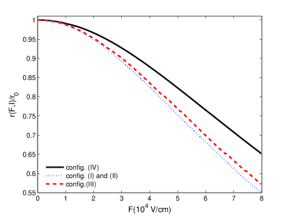
Figure 1: (Color online) Recombination coefficient $r(F,I)/r(0,I)$ vs electric field $F$ for the four configurations listed in Table 1.

III Dimensionless equations

To study the model described by Eqs. (1)–(7), it is convenient to render them dimensionless. For a fixed value of the photo-excitation intensity $I$ and a constant electric field $F_{i}=F$, the stationary solution of Eq. (3) is $n_{i}=p_{i}=\sqrt{\gamma(I)/r(F,I)}$. We use the maximum values $[n]=[p]=\sqrt{\gamma(I)/r(0,I)}$ to define typical values for $n_{i}$ and $p_{i}$. The field $F_{M}$ at the maximum of the drift velocity is a typical value of the field when there are SSOC. Therefore, we adopt it as the field unit $[F]=F_{M}$. Similarly, $[v]=v_{M}$ and, therefore, $[J]=e[n]v_{M}/l$ and $[D]=lv_{M}$. There are two possible time scales, the first one being $t_{F}=\varepsilon F_{M}/[J]$, which balances Maxwell’s displacement current with the current density in Eq. (2), and the second one $t_{n}=[p]/\gamma(I)=1/\sqrt{\gamma(I)r(0,I)}$, which balances both sides of Eq. (3). It is reasonable to choose the time unit as the longer of the two times $t_{F}$ and $t_{n}$. We have chosen four representative GaAs/Al_xGa_1-xAs SL configurations with 10 nm wells and 4 nm barriers. The configurations are I: $x=0.25$ and $I=120.5$ kW/cm²; II: $x=0.25$ and $I=302.69$ kW/cm²; III: $x=0.3$ and $I=479.735$ kW/cm²; and IV: $x=1.0$ and $I=30.27$ kW/cm². We assume a circular cross section with a diameter of 160 $\mu$m, a photo-excitation intensity of 60 mW, a wavelength of 413 nm, and four different beam diameters yielding the previously listed values of the laser intensity. For most of the cases listed in Table 1, $t_{n}>t_{F}$, and therefore we choose $[t]=t_{n}$. All scaled variables are listed in Table 1.

Table 1: Units used to achieve a set of equations with dimensionless variables.

config.	$x$	$I$	$n$, $p$	$F$, $\phi$	$t$	$v$	$J$	$D$	$r$	$\sigma$
			$\sqrt{\frac{\gamma(I)}{r(0,I)}}$	$F_{M}$	$\frac{[n]}{\gamma(I)}$	$v_{M}$	$\frac{e[n]v_{M}}{l}$	$lv_{M}$	$r(0,I)$	$\frac{ev_{M}[n]}{F_{M}l}$
		$\frac{\mbox{kW}}{\mbox{cm}^{2}}$	$\frac{10^{12}}{\mbox{cm}^{2}}$	$\frac{\mbox{kV}}{\mbox{cm}}$	$10^{-11}$ s	$\frac{\mbox{km}}{\mbox{s}}$	$10^{4}\frac{\mbox{A}}{\mbox{cm}^{2}}$	$10^{-2}\frac{\mbox{cm}^{2}}{\mbox{s}}$	$10^{-3}\frac{\mbox{cm}^{2}}{\mbox{s}}$	$\frac{\mbox{A}}{\mbox{V cm}}$
I	0.25	120.5	1.017	16.8	4.602	2.569	2.991	35.97	5.7	1.78
II	0.25	302.69	4.0504	14.72	18.321	0.0057	11.910	35.97	0.90026	7.0891
III	0.3	479.735	8.070	16.0	69.485	1.421	13.12	19.89	0.359	8.912
IV	1	30.27	0.2731	14.72	313.45	0.0057	8.28$\times 10^{-4}$	7.95$\times 10^{-4}$	90.7	5.62$\times 10^{-4}$

We now rewrite the model equations using dimensionless variables by defining $\hat{n}_{i}=n_{i}/[n]$, $\hat{t}=t/[t]$, …, where $[n]$, $[t]$, etc. are the scales defined above and specified in Table 1. Omitting hats over the variables, the dimensionless system of equations corresponding to Eqs. (1)–(7) read

$$F_{i}-F_{i-1}=(n_{i}-p_{i})\nu\;,$$ (10)

$$\delta\,\frac{dF_{i}}{dt}+n_{i}v(F_{i})-D(F_{i})\,(n_{i+1}-n_{i})=J(t)\;,$$ (11)

$$\frac{dp_{i}}{dt}=1-r(F_{i})\,n_{i}p_{i}\;,$$ (12)

$$\sigma\,F_{0}+\delta\,\frac{dF_{0}}{dt}=J\;,\quad\quad\sigma\alpha\,n_{N}F_{N}+\delta\,\frac{dF_{N}}{dt}=J\;,$$ (13)

$$\frac{1}{N+1}\sum_{i=0}^{N}F_{i}=\phi\;,$$ (14)

$$J=\frac{1}{N+1}\sum_{i=0}^{N}J_{i\to i+1}+\frac{d\phi}{dt}\;.$$ (15)

In these equations, there are four dimensionless parameters,

$$\delta=\frac{\varepsilon F_{M}lr(0,I)}{ev_{M}},\quad\nu=\frac{e[n]}{\varepsilon F_{M}},\quad\alpha=\frac{[n]}{N_{D}}\equiv\frac{\sqrt{\gamma(I)}}{N_{D}\sqrt{r(0,I)}}\;,$$ (16)

and the dimensionless conductivity $\hat{\sigma}$, which is here simply denoted by $\sigma$. The values of the dimensionless parameters for the four SL configurations given in Table 1 are listed in Table 2. It is interesting to note that $r(0,I)\propto I^{-2}$ and $\gamma(I)\propto I$ so that $\nu\propto I^{3/2}$ and $\delta\propto I^{-2}$, i.e. $\nu$ increases with photo-excitation intensity, whereas $\delta$ decreases. High photo-excitation intensities imply that $\nu$ is large and $\delta$ small, whereas the opposite holds for low photo-excitation intensities.

Table 2: Numerical values of the dimensionless parameters $\alpha$, $\delta$, $\nu$ and $\hat{\sigma}$ for the four superlattice configurations listed in Table 1.

config.	$\alpha$	$\delta$	$\nu$	$\hat{\sigma}$
	$\frac{[n]}{N_{D}}$	$\frac{\varepsilon F_{M}l\,r(0,I)}{ev_{M}}$	$\frac{e[n]}{\varepsilon F_{M}}$	$\frac{\sigma F_{M}l}{ev_{M}[n]}$
I	0.9713	0.0037	8.446	1.0834
II	0.6944	$5.91\times 10^{-4}$	33.6228	1.0523
III	0.9779	$4.05\times 10^{-5}$	70.507	1.1074
IV	1.5754	22.3714	1.2721	1.2959

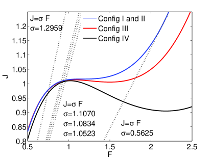
Figure 2: (Color online) Local current density $j$ vs electric field $F$. For a fixed value of the total current density $J$, there may be one or three zeros of $j(F)$-$J$ depending on the Al content $x$.

It is interesting to depict the phase plane corresponding to spatially uniform solutions of Eqs. (10)–(12) with $n_{i}=p_{i}=p$, $F_{i}=F$

$$\delta\,\frac{dF}{dt}=J-p\,v(F),\quad\frac{dp}{dt}=1-r(F)\,p^{2}\;.$$ (17)

Generically and for a fixed value of $J$, the nullclines $v(F)\,p=J$ and $r(F)\,p^{2}=1$ intersect in one or three fixed points, depending on the Al content $x$ in the barriers. At these fixed points,

$$j(F)=J,\quad j(F)=\frac{v(F)}{\sqrt{r(F)}}\;.$$ (18)

The function $j(F)$ is depicted in Fig. 2 for the SL configurations listed in Table 1.

The calculations for arbitrary values of Aluminum content $x$ show that for $0.45\leq x\leq 1$, there are three fixed points of the system in Eq. (17), one on each of the three branches of $p=J/v(F)$, and the ratio of $(j_{\rm max}-j_{\rm min})$ to the average current $(j_{\rm max}+j_{\rm min})/2$ is sufficiently large. As we shall see later, some nonlinear phenomena occurring in these SLs are quite similar to the ones observed in doped SLs: static electric-field domains with domain walls joining the stable branches of $p=J/v(F)$, SSOC due to the recycling of pulses formed by two moving domain walls having a high-field region between them, etc. For $0<x<0.45$, $j(F)$ is either increasing for positive $F$ (for $0<x<0.25$) or the ratio of $(j_{\rm max}-j_{\rm min})$ to the average current $(j_{\rm max}+j_{\rm min})/2$ is small (for $0.25<x<0.45$). For $0<x<0.25$, there is a unique fixed point at $F=F_{*}$, which, for an appropriate value of $J$, may be located on any of the three branches of $p=J/v(F)$. If the fixed point is located on one of the two stable branches of $p=J/v(F)$ for which $v(F)$ has a positive slope, the dynamical system of Eq. (17) is excitable, whereas it is oscillatory if the fixed point is located on the second branch of $p=J/v(F)$ with $v^{\prime}(F_{*})<-2\delta r(F_{*})<0$. In an excitable dynamical system, an appropriate finite disturbance of the unique stable fixed point may cause a large excursion in phase space before returning to the stable state. When diffusion is added, the resulting excitable reaction-diffusion system may support a variety of wave fronts, pulses and wave trains.Kee98 ; Car03 ; Car05 ; Bon09 A dynamical system having an unstable fixed point and a stable limit cycle around it is oscillatory. Again in the presence of diffusion, oscillatory systems may support different spatio-temporal patterns.Kee98 ; Bon09 ; Kur03 An undoped photo-excited SL with excitable or oscillatory dynamics exhibits quite unusual phenomena. Under dc current bias, it is possible to have pulses moving to the right or to the left and periodic wave trains. Under dc voltage bias, these pulses and wave trains may give rise to a variety of SSCOs. Similar phenomena are observed in the case $0.25<x<0.45$ for which $j(F)$ has a shallow valley for a narrow interval of current densities.

IV dc voltage-biased superlattice for small photo-excitation intensities

The behavior of a dc voltage-biased SL is quite different depending on its Al content and photo-excitation intensity. For an Al content smaller than 45%, $j(F)$-$J$ in Eq. (18) has a single zero for any value of $J$, and the only stable states of the SL are stationary ones unless the photo-excitation intensity is sufficiently large (cf. next section). Let us assume that the Al content is larger than 45% so that $j(F)$-$J$ in Eq. (18) may have three zeros for an appropriate range of $J$ values. In this case, the undoped SL behaves similarly to an $n$-doped SL.Bon05 The most interesting limit is that of small photo-excitation intensity, i. e., $\delta\gg 1$.

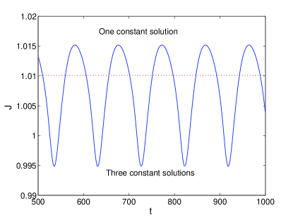
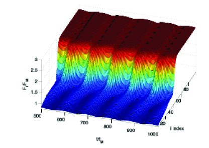
Figure 3: (Color online) Current vs time (top) and field distribution vs time (bottom) displaying SSCOs due to monopole recycling at the injecting contact. The injecting contact conductivity and the bias are $\sigma=1.2959$ and $V=2.0416236$, respectively. The other parameter values correspond to configuration IV in Table 1 and are $N=99$, $\delta=22.35636$, $\sigma_{2}=1.3148$, $\nu=1.27214$, and Al content $x=1$.

For the time scale $\tau=t/\delta$, Eqs. (11) and (12) can be rewritten as

$$\frac{dF_{i}}{d\tau} = J-\left(p_{i}+\frac{F_{i}-F_{i-1}}{\nu}\right)v(F_{i})$$ (19)

$$+ \left(p_{i+1}-p_{i}+\frac{F_{i+1}+F_{i-1}-2F_{i}}{\nu}\right)D(F_{i})\;,$$

$$\delta^{-1}\frac{dp_{i}}{d\tau} = 1-\left(p_{i}+\frac{F_{i}-F_{i-1}}{\nu}\right)p_{i}\,r(F_{i})\;.$$ (20)

In the limit of large photo-excitation intensities, $\delta\ll 1$, Eq. (20) indicates that the $p_{i}$ do not depend on $\tau$. In this case, Eq. (19) corresponds to a SL doped with a density $p_{i}$, and we may expect phenomena similar to the ones observed in an $n$-doped SL. In the opposite limit of small photo-excitation intensities, $\delta^{-1}\ll 1$, $\tau=\delta^{-1}t$ is a slow scale. The $p_{i}$ are functions of $F_{i}-F_{i-1}$ determined by solving Eq. (20) with a zero left hand side

$$p_{i}=\sqrt{\left(\frac{F_{i}-F_{i-1}}{2\nu}\right)^{2}+\frac{1}{r(F_{i})}}-\frac{F_{i}-F_{i-1}}{2\nu}\;.$$ (21)

The resulting equation for $F_{i}$ is then obtained by inserting Eq. (21) into Eq. (19)

$$\frac{dF_{i}}{d\tau} = J-\left(\sqrt{\left(\frac{F_{i}-F_{i-1}}{2\nu}\right)^{2}+\frac{1}{r(F_{i})}}+\frac{F_{i}-F_{i-1}}{2\nu}\right)v(F_{i})$$ (22)

$$+ \left[\sqrt{\left(\frac{F_{i+1}-F_{i}}{2\nu}\right)^{2}+\frac{1}{r(F_{i+1})}}-\sqrt{\left(\frac{F_{i}-F_{i-1}}{2\nu}\right)^{2}+\frac{1}{r(F_{i})}}\right.$$

$$+ \left.\frac{F_{i+1}+F_{i-1}-2F_{i}}{2\nu}\right]D(F_{i})\;.$$

This equation is similar to the one describing the electric field in a doped SL, but now there are drift and diffusion terms which are nonlinear in the differences $F_{i}-F_{i-1}$. Under dc voltage bias, there are SSOC mediated by pulses of the electric field. The current density varies on a slow time scale, whereas the electric-field profile consists of a varying number of wave fronts joining the stable constant solutions of Eq. (22) at the instantaneous value of the current.Bon05 Depending on the conductivity of the injecting contact $\sigma$, there are different types of SSOC due to the periodic generation of dipoles or monopoles at the injecting contact. If the curve $\sigma F$ intersects the bulk current-field characteristic curve $j(F)$ before its maximum (cf. Fig. 2), SSCOs due to recycling and motion of charge monopole waves (moving charge accumulation layers) appear as shown in Fig. 3. If $\sigma F$ intersects $j(F)$ after its maximum (cf. Fig. 2), SSCOs due to recycling and motion of dipole waves are obtained, as depicted in Fig. 4. We have indicated in Figs. 3 and 4 whether there are one or three uniform and time-independent (constant) solutions of Eq. (17), solving $p\,v(F)=J$ and $r(F)\,p^{2}=1$ for the instantaneous value of the current density $J=J(t)$ during the SSOC.

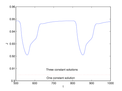
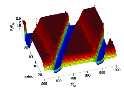
Figure 4: (Color online) Current vs time (top) and field distribution vs time (bottom) displaying SSCOs due to dipole recycling at the injecting contact. The injecting contact conductivity and the bias are $\sigma=0.5625$ and $V=2.05148375$, respectively. The other parameter values are the same as the ones used for Fig. 3 corresponding to configuration IV in Table 1.

V dc voltage-biased superlattice for large photo-excitation intensities

If $0<x<0.45$, the phase plane in Eq. (17) may have only one fixed point located on any branch of the nullcline $p=J/v(F)$. For small photo-excitation intensities, the only stable state is a stationary one. However, for sufficiently large photo-excitation intensities, an infinite, dc current-biased SL may exhibit pulses moving downstream or upstream and also wave trains moving downstream.abg_math The counterpart of these stable solutions for a dc voltage-biased SL is very interesting and different from anything observed in an $n$-doped SL. Our simulations correspond to SLs with different Al contents, whose current-field characteristics $j(F)$ and injecting contact curve $j=\sigma F$ are shown in Fig. 2. In all cases, SSCOs appear for an average bias roughly in the region of negative differential resistance (NDR), where $j^{\prime}(F)<0$ (e.g., $\sigma$=0.5625 in Fig. 2).

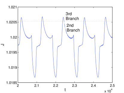
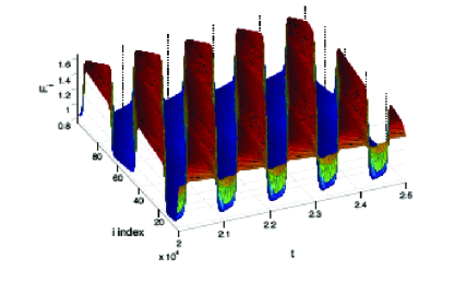
Figure 5: (Color online) Current vs time (top) and field distribution vs time (bottom) displaying dipole-mediated bulk SSCOs for an injecting contact conductivity $\sigma=1.05231$ and $x=0.25$ (cf. Fig. 2). These oscillations correspond to having a finite wave train. The other parameter values correspond to configuration II in Table 1 and are $N=99$, $\nu=33.62275$, $\delta=5.91\times 10^{-4}$, $V=1.22732$, and $\sigma_{2}=0.73075$.

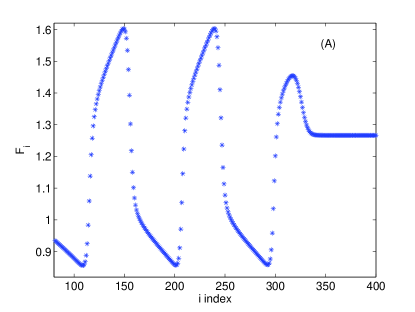
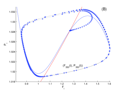
Figure 6: (Color online) (a) Numerically obtained field profile of a pulse moving with positive speed followed by a wave train when there is only one critical point in the phase plane. (b) Phase plane showing the nullclines and the motion of the 350th QW as the pulse traverses it. The total current density is $J=1.0165$ and the other parameters correspond to configuration I in Table 1.

When the conductivity of the injecting contact is such that $\sigma F$ intersects $j(F)$ near the maximum thereof, it is possible to have SSCOs that are quite different from the ones appearing in $n$-doped SLs. For an injecting contact conductivity $\sigma=1.05231$ (cf. Fig. 2), pulses (charge dipoles) may be triggered at the injecting contact, move toward the receiving contact, and cause SSCOs as shown in Fig. 5. For all the instantaneous values of $J(t)$ during these SSCOs, there is only one constant solution of Eq. (17): most of the times this solution is on the second NDR branch of $j(F)$. Only when $J(t)$ is near its maximum value, the constant solution is on the third branch of $j(F)$. For a constant current density, the constant solution of Eq. (17) is on the NDR branch, which implies that the system is oscillatory and that periodic wave trains are possible. The realization of wave trains for a long dc-biased SL are displayed in Fig. 6: at any time during SSOC, there are only two fully developed pulses present in this SL. These pulses experience variations in their shape and velocity when they are generated or arrive at the contacts, but longer SLs allow for realizations of wave trains, in which more pulses exist simultaneously inside the SL.

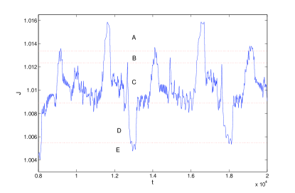
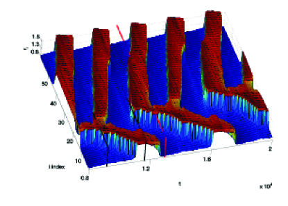
Figure 7: (Color online) Current vs time (top) and field distribution vs time (bottom) displaying dipole-mediated bulk SSCOs for an injecting contact conductivity $\sigma=1.107$ (cf. Fig. 2). The other parameter values correspond to configuration III in Table 1 and are $N=61$, $\nu=70.50677$, $\delta=4.069\times 10^{-4}$, $V=1.269848$, and $\sigma_{2}=1.0829727$.

In the previous example, pulses always move downstream, from left to right. For slightly larger conductivity of the injecting contact ($\sigma=1.107$ in Fig. 2), Fig. 7 shows that two pulses are formed inside the SL and move with opposite velocities toward the contacts. These pulses are similar to the ones constructed above for the case of dc current bias (with positive or negative velocity), except that the current changes slowly with time during the self-oscillation and the pulses accommodate their form to the instantaneous value of the current. Note that the pulses are triggered inside the SL, not at the injecting contact. A pulse moving with positive speed has a long trailing region, in which the field increases as we move away from the pulse. However, there is a depletion layer near the injecting contact, in which the field decreases as we move away from the injecting contact. In a long, but finite SL, a local maximum is formed inside the SL, when the decreasing field near the contact meets the increasing field in the trailing region of the exiting pulse with positive speed. The current increases as the exiting pulse is absorbed by the receiving contact, until it surpasses a critical value. In this case, the local maximum of the field profile inside the SL is split, and two new pulses are created. The pulse closer to the injecting contact moves toward it with negative speed whereas the other pulse moves toward the receiving contact with positive speed. The upward moving pulse reaches the injecting contact and is absorbed there before the downward moving pulse arrives at the other contact. In this case, the field profile close to the injecting contact is quasi-stationary, and a local maximum of the field is formed when we match this region with the trailing region of the downward moving pulse. After the critical value of the current is reached, another pulse pair is nucleated, and the same process is periodically repeated.

It is interesting to evaluate in some detail the process of nucleation and disappearance of pulses during these SSCOs. In the current vs time diagram in Fig. 7, we distinguish different regions depending on the number of constant solutions of Eq. (17) that exist for the corresponding instantaneous value of $J(t)$. In region A, there is only one constant solution on the third branch of $j(F)$. In region B, there is one constant solution on the third branch and two on the second branch of $j(F)$. In region C, there are three constant solutions, one on each branch of $j(F)$, whereas two of these solutions are on the second branch and one of the first branch of $j(F)$, if $J(t)$ is in region D. There is only one constant solution located on the first branch of $j(F)$, if $J(t)$ is in region E. For a constant voltage bias, a pulse moving upstream may be generated only if $J(t)$ surpasses a critical value (1.007454), which is located in region C and marked by an arrow. Once generated, the upstream moving pulses persist for any instantaneous value of the current density. These SSOC are apparently weakly chaotic: we have calculated the corresponding Lyapunov exponents and found that there is a single positive exponent with a rather small value of $7.9$$\times$$10^{-6}$.

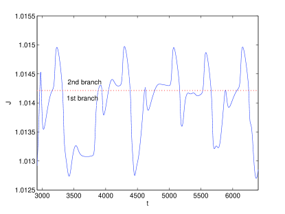
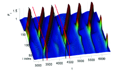
Figure 8: (Color online) Current vs time (top) and field distribution vs time (bottom) displaying dipole-mediated bulk SSCOs for an injecting contact conductivity $\sigma=1.083425$ (cf. Fig. 2). The other parameter values correspond to configuration I in Table 1 and are $N=199$, $\nu=8.44566$, $\delta=3.7287\times 10^{-3}$, $V=1.00417485$, and $\sigma_{2}=1.0523129$.

We have also observed SSCOs mediated by dipole waves that nucleate alternatively at two different QWs of the SL as shown in Fig. 8. During these SSCOs, there is only one constant solution of Eq. (17) for any instantaneous value of $J(t)$. This solution is either on the first or the second branch of $j(F)$. At about $t=3232$, where $J(t)$ reaches its global maximum, two dipole waves are nucleated at two different QWs. They become fully developed pulses and move with positive speed toward the receiving contact. When the first one arrives there, the current increases so that the corresponding constant solution of Eq. (17) is on the second branch of $j(F)$. In this case, a small dipole wave is nucleated at the local field maximum, where the tail of the first dipole meets the depletion layer near the injecting contact. The small dipole wave never grows into a fully developed field pulse, and it continues advancing, until the old large dipole wave disappears at the receiving contact. At this time (about 4296), a large current spike appears, and a new dipole wave is formed closer to the injecting contact than the small dipole. $J(t)$ decreases abruptly, while the small dipole disappears, and the newly created dipole reaches a large size and moves toward the receiving contact. Shortly afterward, a new current spike marks the creation of another small dipole. This small dipole travels toward the receiving contact, and it grows only when the only existing large pulse reaches the receiving contact and disappears. A small dipole formed closer to the injecting contact does not grow, until the large pulse reaches the receiving contact and disappears without triggering a new dipole wave. In this case, the corresponding pulse is close to the receiving contact. When it reaches the contact and disappears into it, two new dipoles are simultaneously triggered and become fully developed. A scenario similar to the one previously described follows, marked again by a large current spike. The situation is not repeated exactly: there are small differences in the QWs at which pulses are nucleated, differences in the size and lifetimes of the small dipoles, etc. These oscillations also seem to be weakly chaotic, in which a single Lyapunov exponent is small and positive.

If the injecting contact conductivity is smaller so that the contact current $\sigma F$ intersects $j(F)$ on the NDR branch thereof, there appear standard SSCOs due to repeated dipole pulse nucleation at the injecting contact and motion toward the receiving contact.

VI Conclusions

We have calculated the recombination coefficient as a function of the applied electric field for undoped, photo-excited, weakly coupled GaAs/Al_xGa_1-xAs superlattices. Depending on the Al content $x$, the superlattice may have only one static domain for small $x$ or two stable differentiated static domains for $0.45<x\leq 1$. In the latter case, a dc voltage biased SL under weak photoexcitation may exhibit self-sustained oscillations of the current due to repeated nucleation of a charge monopole or dipole waves at the injecting contact and their motion toward the collector. For high photo-excitation intensities, the walls separating electric field domains are mostly pinned, and self-sustained oscillations of the current occur only in narrow voltage intervals. For small $x$ among other unusual phenomena, there may appear weakly chaotic SSOC due to dipole dynamics in dc-voltage-biased SLs for high photo-excitation intensities, during which nucleated dipole waves can split in two oppositely moving dipoles. These dipoles are pulses of the electric field with shapes and behavior similar to pulses in excitable media, where a sufficiently large disturbance about the unique stable domain may induce them. For other parameter values, the unique static domain is unstable, and the underlying dynamics is oscillatory so that wave trains formed by succession of pulses give rise to self-sustained oscillations of the current.

References

- (1) L. L. Bonilla, J. Galán, J. A. Cuesta, F. C. Martínez, and J. M. Molera, Phys. Rev. B 50, 8644 (1994).
- (2) L. L. Bonilla, in Nonlinear Dynamics and Pattern Formation in Semiconductors and Devices, edited by F.-J. Niedernostheide. Page 1. Springer, Berlin, 1995.
- (3) H. T. Grahn, H. Schneider, and K. von Klitzing, Phys. Rev. B 41, 2890 (1990).
- (4) S. H. Kwok, T. B. Norris, L. L. Bonilla, J. Galán, J. A. Cuesta, F. C. Martínez, J. M. Molera, H. T. Grahn, K. Ploog, and R. Merlin, Phys. Rev. B 51, 10171 (1995).
- (5) M. Hosoda, H. Mimura, N. Ohtani, K. Tominaga, T. Watanabe, K. Fujiwara, and H. T. Grahn, Appl. Phys. Lett. 69, 500 (1996).
- (6) N. Ohtani, M. Hosoda, and H. T. Grahn, Appl. Phys. Lett. 70, 375 (1997).
- (7) A. M. Tomlinson, A. M. Fox, J. E. Cunningham, and W. Y. Jan, Appl. Phys. Lett. 75, 2067 (1999).
- (8) K. J. Luo, S. W. Teitsworth, H. Kostial, H. T. Grahn, and N. Ohtani, Appl. Phys. Lett. 74, 3845 (1999).
- (9) N. Ohtani, N. Egami, K. Fujiwara, and H. T. Grahn, Solid-State Electron. 42, 1509 (1998).
- (10) L. L. Bonilla and H. T. Grahn, Rep. Prog. Phys. 68, 577 (2005).
- (11) A. Perales, L. L. Bonilla, M. Moscoso, and J. Galán, Int. J. Bifurcations and Chaos 11, 2817 (2001).
- (12) J. P. Keener and J. Sneyd, Mathematical Physiology (Springer, New York, 1998).
- (13) A. Carpio and L. L. Bonilla, SIAM J. Appl. Math. 63, 619 (2003).
- (14) A. Carpio, Physica D 207, 117 (2005).
- (15) L. L. Bonilla and S. W. Teitsworth, Nonlinear wave methods for charge transport (Wiley, New York), to appear.
- (16) H. T. Grahn, Introduction to Semiconductor Physics (World Scientific, Singapore, 1999).
- (17) Y. Kuramoto, Chemical oscillations, waves and turbulence (Dover, New York, 2003).
- (18) J. I. Arana, L. L. Bonilla, and H. T. Grahn, unpublished.