Nonparametric Bayesian Density Modeling with Gaussian Processes

Abstract

We present the Gaussian process density sampler (GPDS), an exchangeable generative model for use in nonparametric Bayesian density estimation. Samples drawn from the GPDS are consistent with exact, independent samples from a distribution defined by a density that is a transformation of a function drawn from a Gaussian process prior. Our formulation allows us to infer an unknown density from data using Markov chain Monte Carlo, which gives samples from the posterior distribution over density functions and from the predictive distribution on data space. We describe two such MCMC methods. Both methods also allow inference of the hyperparameters of the Gaussian process.

journalname

, and

t1Supported by the Canadian Institute for Advanced Research.

1 Introduction

We propose a method for incorporating a Gaussian process into a prior on probability density functions. While such constructions have been proposed before (Leonard, 1978; Thorburn, 1986; Lenk, 1988, 1991; Csató, 2002; Tokdar and Ghosh, 2007; Tokdar, 2007), ours is the first that allows a procedure for drawing exact and exchangeable data samples from a density drawn from the prior. We call this prior and the associated procedure the Gaussian process density sampler (GPDS). Given data, this generative prior allows us to perform inference of the unnormalised density. We present two Markov chain Monte Carlo (MCMC) algorithms for performing this inference, one based on exchange sampling (Murray et al., 2006) and the other based on inferring the latent generative history. In both cases we are also able to infer the parameters governing the covariance kernel, and draw samples from the predictive distribution on data space.

Bayesian nonparametric inference is appealing because it allows models to include an arbitrary number of parameters, without requiring expensive dimensionality-altering computations for inference. The most popular tool for nonparametric Bayesian modeling of an unknown probability measure is the Dirichlet process (Ferguson, 1973) and related constructions (e.g., Pitman and Yor (1997) and Ishwaran and James (2001)). Samples from the Dirichlet process, however, are discrete distributions with probability one. For many inference problems, we wish to model probabilities on continuous spaces and in such problems our prior beliefs are often best captured by a distribution over probability density functions.

To fill the gap between nonparametric priors on discrete distributions and nonparametric priors on continuous densities, the Dirichlet process is frequently used to add a countably-infinite number of parameters into a continuous model. The most popular example is the infinite mixture of parametric distributions (Escobar and West, 1995), another example is kernel convolution (Lo, 1984). The Dirichlet diffusion tree (Neal, 2001, 2003) and Pólya trees (Lavine, 1992, 1994) provide more direct nonparametric priors on distributions and, in contrast to the Dirichlet process, can produce densities. All of these priors are based on beliefs of an underlying structure, either a clustering or tree-based hierarchy.

Prior beliefs about a distribution over data are sometimes best expressed directly in terms of the probability density function — its continuity, support and smoothness properties, for example. There is a rich literature on incorporating prior beliefs about functions into nonparametric Bayesian regression models, using splines, neural networks and stochastic processes (e.g., DiMatteo et al. (2001), MacKay (1992), and O’Hagan (1978)). However, priors on general functions have largely resisted application to density estimation, due to the requirements that probability density functions be nonnegative and integrate to one. This work introduces the first fully-nonparametric Bayesian kernel method for density estimation that does not require a finite-dimensional approximation to perform inference.

2 The Gaussian process density sampler prior

The GPDS provides a probability distribution on a space $\mathcal{X}$, which we call the data space. In many problems, $\mathcal{X}$ is the $D$-dimensional real space $\mathbb{R}^{D}$.

We first place a Gaussian process prior over a scalar function ${g(\boldsymbol{x}):\mathcal{X}\to\mathbb{R}}$. This means that the prior distribution over any discrete set of function values, $\{g(\boldsymbol{x}_{n})\}_{n=1}^{N}$, is a multivariate normal distribution. These distributions can be consistently defined with a positive definite covariance function ${C(\cdot,\cdot):\mathcal{X}\times\mathcal{X}\rightarrow\mathbb{R}}$ and a mean function ${m(\cdot):\mathcal{X}\rightarrow\mathbb{R}}$. The mean and covariance functions are parameterised by hyperparameters $\theta$. For a more detailed review of Gaussian processes see, e.g., Rasmussen and Williams (2006).

We construct a map from the function $g(\boldsymbol{x})$ to a probability density function $f(\boldsymbol{x})$ via

$$f(\boldsymbol{x}) =\frac{1}{\mathcal{Z}_{\pi}[\boldsymbol{g}]}\,\Phi(g(\boldsymbol{x}))\,\pi(\boldsymbol{x}\,|\,\psi)$$ (2.1)

where $\pi(\boldsymbol{x}\,|\,\psi)$ is a parametric base density that corresponds to an arbitrary base probability measure on $\mathcal{X}$, with hyperparameters $\psi$. The function ${\Phi(\cdot):\mathbb{R}\rightarrow(0,1)}$ is a positive function with upper bound $1$. We use the bold notation $\boldsymbol{g}$ to refer to the function $g(\boldsymbol{x})$ compactly as a vector of (infinite) length on which it is possible to perform inference. The normalisation constant $\mathcal{Z}_{\pi}[\boldsymbol{g}]$ is a functional of $g(\boldsymbol{x})$:

$$\mathcal{Z}_{\pi}[\boldsymbol{g}] =\int\!\mathrm{d}x^{\prime}\;\Phi(g(x^{\prime}))\,\pi(x^{\prime}\,|\,\psi).$$ (2.2)

We include the subscript $\pi$ to indicate implicit dependence on the density $\pi(\boldsymbol{x})$. Through the map defined by Equation 2.1, a Gaussian process provides a prior distribution over normalised probability density functions on $\mathcal{X}$. Figure 1 shows several realisations of densities from this prior, along with sample data.

Although we only require that the function $\Phi(\cdot)$ be positive and bounded, it is convenient for inference if it is a bijective map between $\mathbb{R}$ and $(0,1)$. If $\Phi(\cdot)$ is bijective then each function that maps $\mathcal{X}$ to $(0,1)$ corresponds to a unique realisation $g(\boldsymbol{x})$ from the Gaussian process. Sigmoids, such as the cumulative normal distribution function and the logistic function, are bijective functions with this domain and range. We take $\Phi(\cdot)$ to be the logistic function, i.e., $\Phi(z)=1/(1+\exp(-z))$.

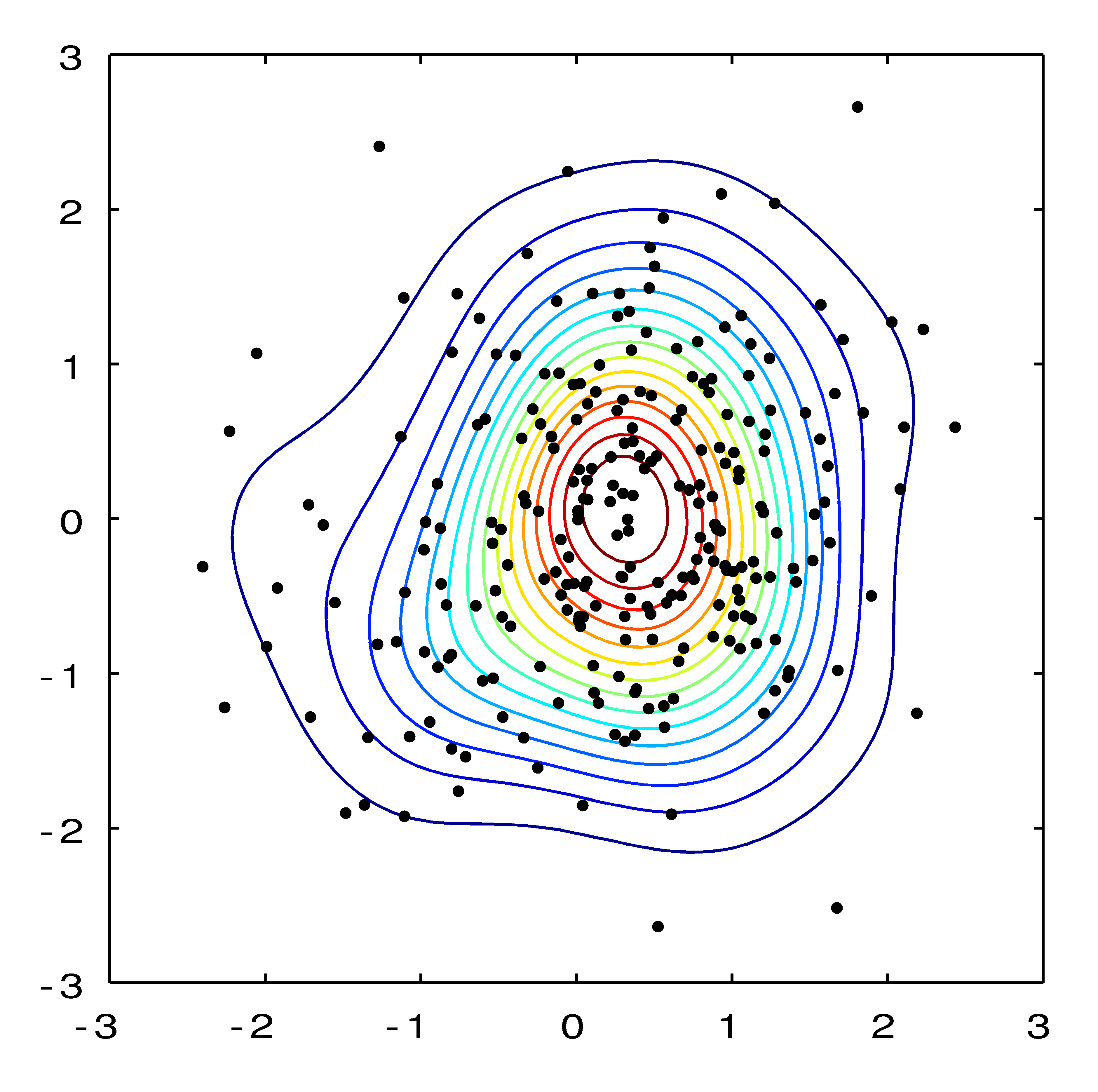
(a)

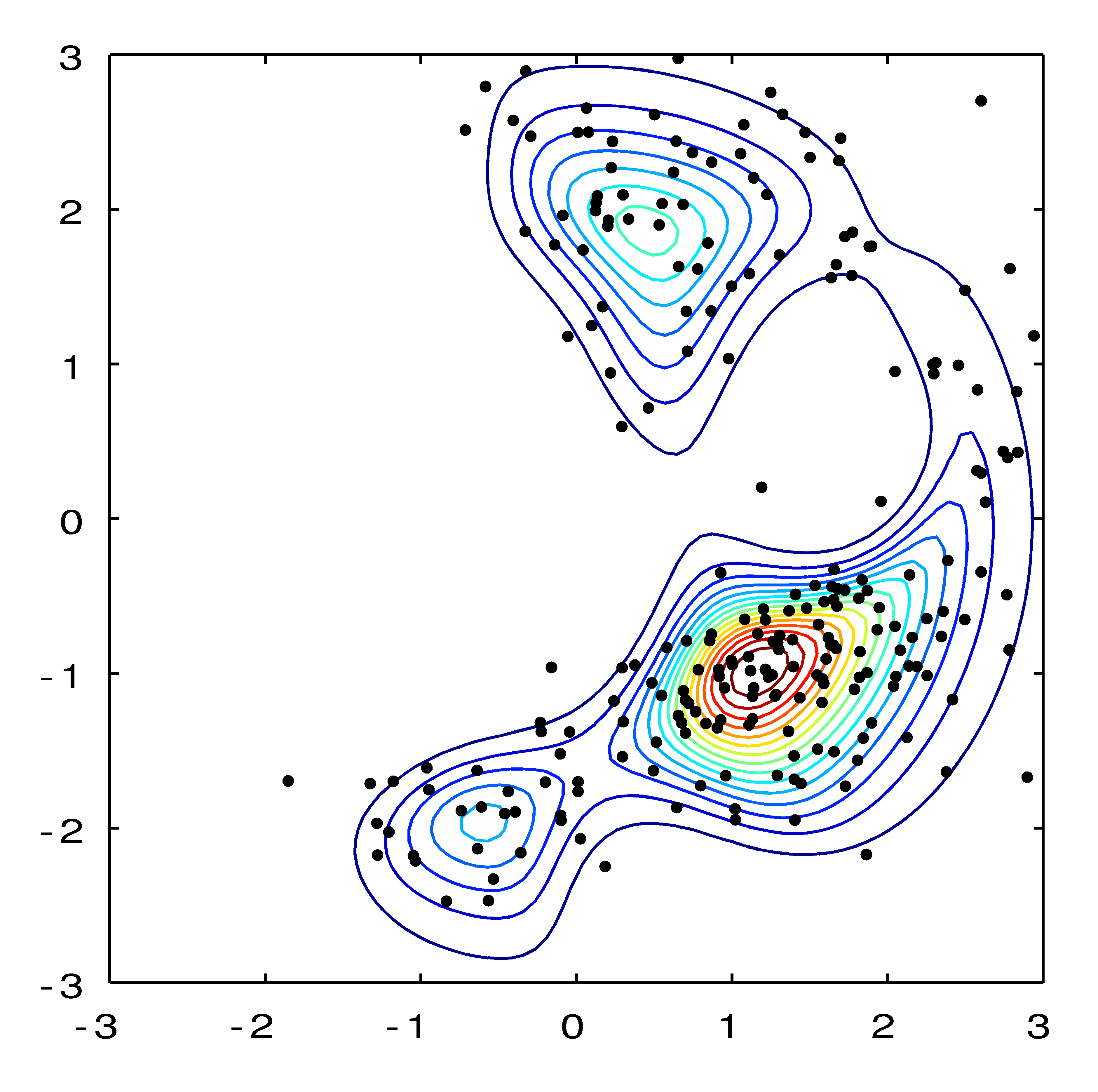
(b)

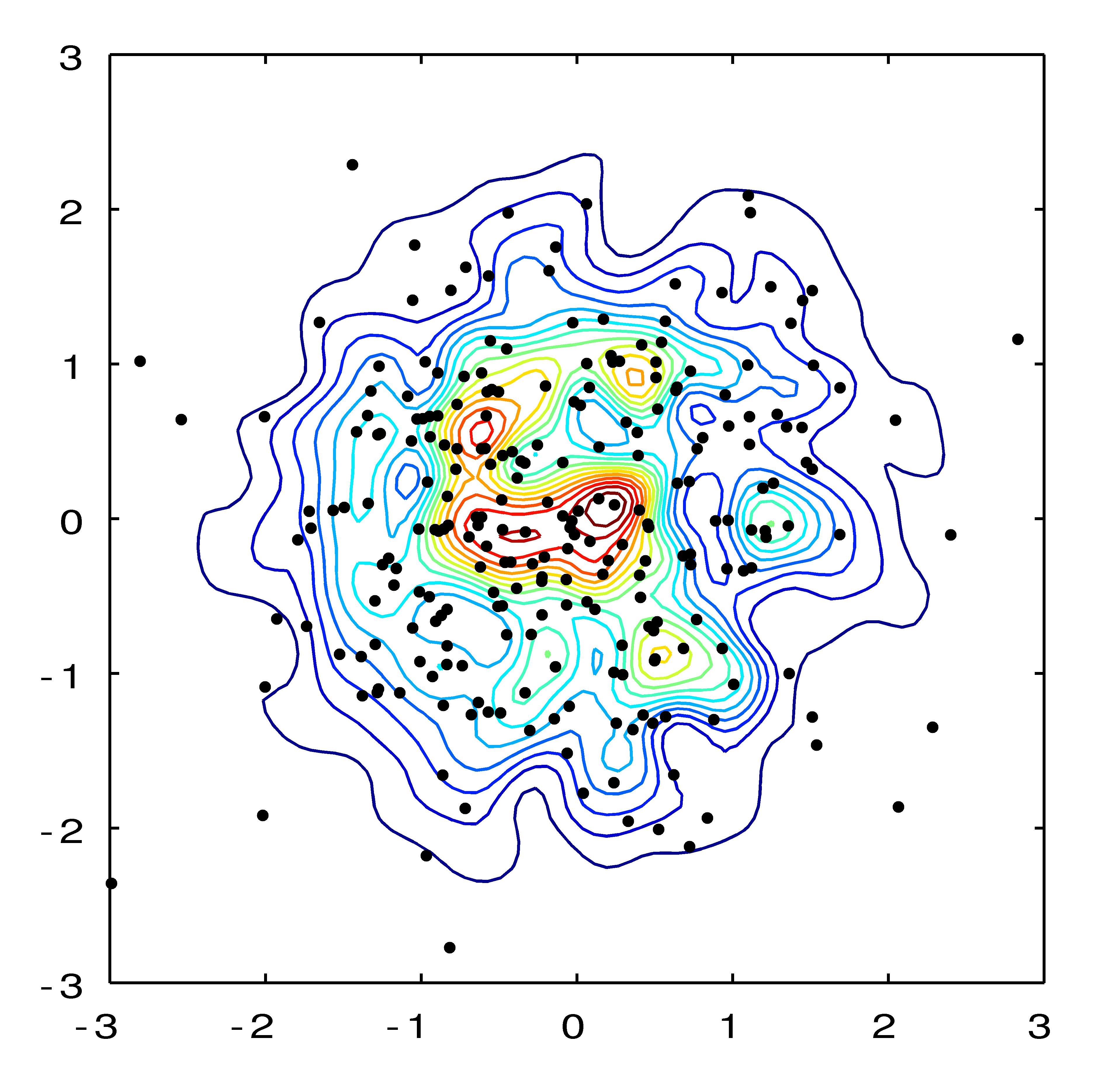
(c)

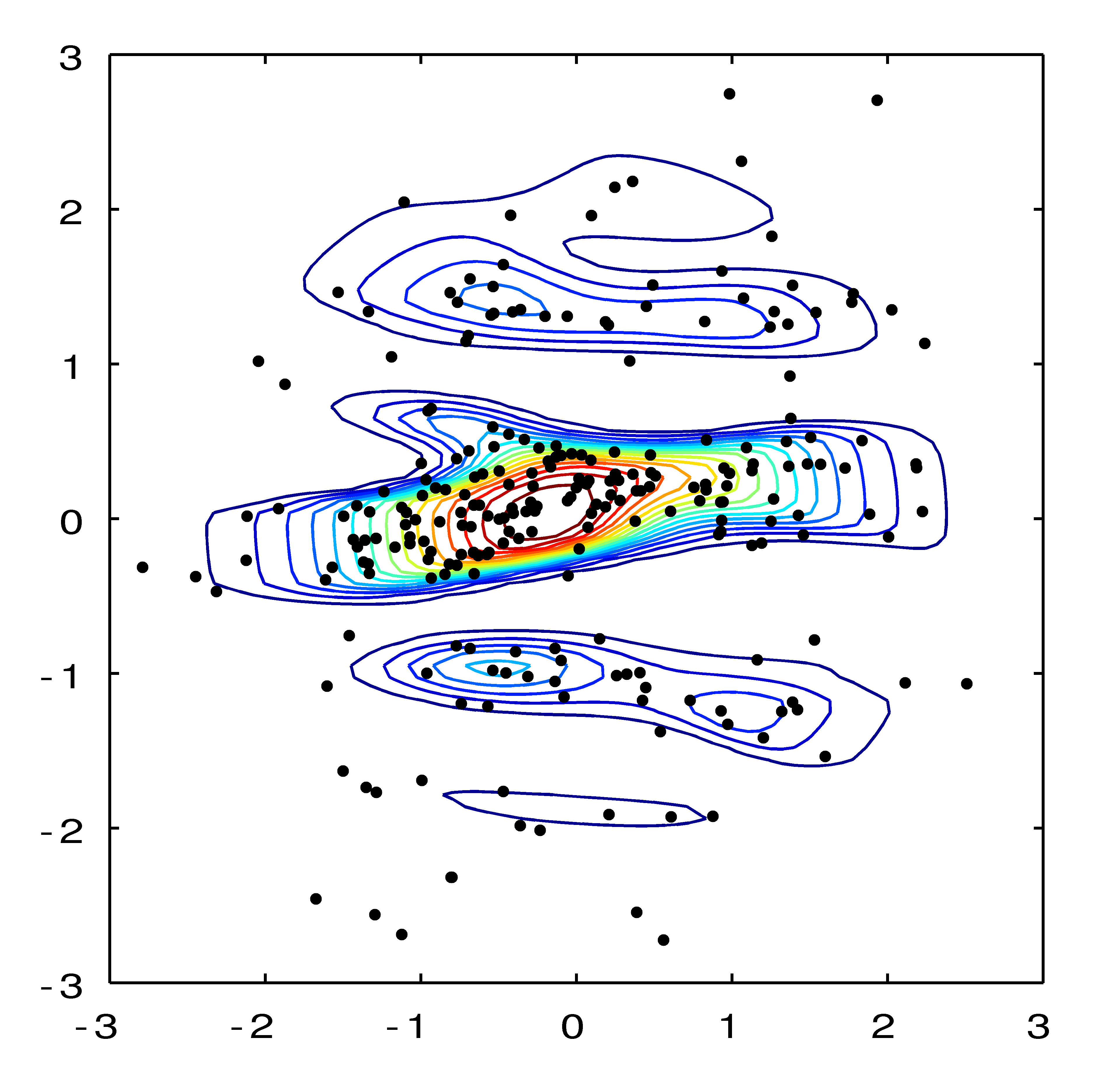
(d)

Figure 1: Four samples from the GPDS prior are shown, with 250 data samples. The contour lines show the approximate unnormalized densities. In each case the base density is the zero-mean circular Gaussian with unit variance. The mean function is set to zero. The covariance function is the squared exponential: $C(\boldsymbol{x},\boldsymbol{x}^{\prime})=\alpha^{2}~{}\exp(-\frac{1}{2}\sum_{d}(x_{d}-x_{d}^{\prime})^{2}/\ell_{d}^{2})$, with parameters varied as labeled in each subplot. $\Phi(\cdot)$ is the logistic function in these plots.

3 Generating data from the prior

We can use rejection sampling to simulate samples from a common density drawn from the the prior described in Section 2. A rejection sampler requires a proposal density that upper bounds the unnormalised density of interest. In this case, the proposal density is $\pi(\boldsymbol{x}\,|\,\psi)$ and the unnormalised density of interest is $\Phi(g(\boldsymbol{x}))\,\pi(\boldsymbol{x}\,|\,\psi)$. We assume that it is possible to draw samples directly from $\pi(\boldsymbol{x}\,|\,\psi)$.

If $g(\boldsymbol{x})$ were known, rejection sampling would proceed as follows: first generate proposals $\{\boldsymbol{\tilde{x}}_{r}\}$ from the base density $\pi(\boldsymbol{x}\,|\,\psi)$. The proposal $\boldsymbol{\tilde{x}}_{r}$ would be accepted if a variate $u_{r}$ drawn uniformly from $(0,1)$ was less than $\Phi(g(\boldsymbol{\tilde{x}}_{r}))$. These samples would be exact in the sense that they were not biased by the starting state of a finite Markov chain. However, in the GPDS, $g(\boldsymbol{x})$ is not known: it is a random function drawn from a Gaussian process prior. We can nevertheless use rejection sampling by “discovering” $g(\boldsymbol{x})$ as we proceed at just the places we need to know it, by sampling from the prior distribution of the latent function. As the values of $g(\boldsymbol{x})$ evaluated at the $\{\boldsymbol{\tilde{x}}_{r}\}$ are consistent with a single draw of the whole function, the samples are exact. This type of retrospective sampling trick has been used in a variety of MCMC algorithms for infinite-dimensional models Beskos et al. (2006); Papaspiliopoulos and Roberts (2008). Figure 2h shows the generative procedure graphically.

(a)

(b)

(c)

(d)

(e)

(f)

(g)

\begin{picture}(1680.0,1680.0)(1.0,-841.0)\end{picture}

(h)

In practice, we generate the samples sequentially, as in Algorithm 3.1, so that we may be assured of having as many accepted samples as we require. In each loop, a proposal is drawn from the base density $\pi(\boldsymbol{x}\,|\,\psi)$ and the function $g(\boldsymbol{x})$ is sampled from the Gaussian process at this proposed coordinate, conditional on all the function values already sampled. We will call these data the conditioning set for the function $g(\boldsymbol{x})$ and will denote the conditioning inputs as X and the conditioning function values as G. After the function is sampled, a variate is drawn uniformly from $(0,1)$ and compared to the $\Phi$-squashed function at the proposal location. If the uniform variate falls below $\Phi(g(\boldsymbol{x}))$ then we accept the proposal, otherwise we reject. The proposals and their function values are added into the conditioning set regardless of whether that proposal was accepted or rejected. The loop repeats until we have as many acceptances as are required.

The sequential procedure is infinitely exchangeable; the probability of the data is the same under reordering. First, the base density draws are i.i.d.. Second, conditioned on the proposals from the base density, the Gaussian process is a simple multivariate Gaussian distribution, which is exchangeable in its components. Finally, conditioned on the draw from the Gaussian process, the acceptance/rejection steps are independent Bernoulli samples, and the overall procedure is exchangeable. This property ensures that the sequential procedure generates data from the same distribution as the simultaneous procedure described above. More broadly, exchangeable priors are useful in Bayesian modeling because we may consider the data conditionally independent, given the latent density.

1:

2:Number of samples to draw $N$

3:Gaussian process covariance function $C(\boldsymbol{x},\boldsymbol{x}^{\prime}\,;\,\theta)$

4:Base density $\pi(\boldsymbol{x}\,|\,\psi)$

5: • $N$ samples $\mathcal{D}=\{\boldsymbol{x}_{n}\}^{N}_{n=1}$ from a random density drawn from the prior.

6:$\textbf{X}\leftarrow\emptyset$, $\textbf{G}\leftarrow\emptyset$ $\triangleright$ Initially the conditioning sets are empty.

7:$\mathcal{D}\leftarrow\emptyset$ $\triangleright$ Initialize the set to be returned.

8:$r\leftarrow 0$ $\triangleright$ Count the number of proposals.

9:repeat

10:     $\boldsymbol{\tilde{x}}_{r}\sim\pi(\boldsymbol{x}\,|\,\psi)$ $\triangleright$ Draw a proposal.

11:     $g(\boldsymbol{\tilde{x}}_{r})\sim\mathcal{GP}(g\,|\,\boldsymbol{\tilde{x}}_{r},\textbf{X},\textbf{G},\theta)$ $\triangleright$ Sample from the GP at the proposal.

12:     $u_{r}\sim\textsf{Un}(0,1)$ $\triangleright$ Draw uniformly on $(0,1)$.

13:     if $u_{r}<\Phi(g(\boldsymbol{\tilde{x}}_{r}))$ then $\triangleright$ Rejection sampling acceptance rule.

14:         $\mathcal{D}\leftarrow\mathcal{D}\cup\boldsymbol{\tilde{x}}_{r}$ $\triangleright$ Store the proposal.

15:     end if

16:     $\textbf{X}\leftarrow\textbf{X}\cup\boldsymbol{\tilde{x}}_{r}$, $\textbf{G}\leftarrow\textbf{G}\cup g(\boldsymbol{\tilde{x}}_{r})$ $\triangleright$ Update the conditioning sets, even on rejections.

17:     $r\leftarrow r+1$

18:until $||\mathcal{D}||=N$ $\triangleright$ Loop until $N$ samples are accepted.

19:return $\mathcal{D}$

Algorithm 3.1 Generate $N$ exact samples from a density drawn from the prior

4 Inference

We now consider the problem of inference with the GPDS. We observe $N$ data $\mathcal{D}=\{\boldsymbol{x}_{n}\}^{N}_{n=1}$ that we model as having been drawn independently from an unknown density $f(\boldsymbol{x})$. We place the GPDS prior of Section 2 on $f(\boldsymbol{x})$. The posterior on $\boldsymbol{g}$ is given by Bayes’ theorem:

$$p(\boldsymbol{g}\,|\,\mathcal{D},\theta) =\frac{p(\boldsymbol{g}\,|\,\theta)\;(\mathcal{Z}_{\pi}[\boldsymbol{g}])^{-N}\prod_{n=1}^{N}\Phi(g(\boldsymbol{x}_{n}))\;\pi(\boldsymbol{x}_{n}\,|\,\psi)}{\int\mathrm{d}\boldsymbol{g}^{\prime}\;p(\boldsymbol{g}^{\prime}\,|\,\theta)\;(\mathcal{Z}_{\pi}[\boldsymbol{g}^{\prime}])^{-N}\prod_{n=1}^{N}\Phi(g^{\prime}(\boldsymbol{x}_{n}))\;\pi(\boldsymbol{x}_{n}\,|\,\psi)}.$$ (4.1)

Even with Markov chain Monte Carlo, inference in this model is difficult. Evaluating the posterior requires computing two difficult integrals, the denominator and the normalisation constant $\mathcal{Z}_{\pi}[\boldsymbol{g}]$. It is common for the marginal likelihood in the denominator of the posterior to be intractable; MCMC methods such as Metropolis–Hastings are well-suited for this situation. Posteriors such as Equation 4.1 with difficult sums in both the numerator and denominator are called doubly-intractable. Doubly-intractable posterior distributions appear most frequently when performing inference in undirected graphical models, where the partition function can be difficult to evaluate (Møller et al., 2006; Murray et al., 2006).

To see the difficulty concretely, consider a naïve Metropolis–Hastings Markov chain on $\boldsymbol{g}$, with proposal density $q(\boldsymbol{\hat{g}}\leftarrow\boldsymbol{g})$:

$$a_{\textsf{na{\"{i}}ve}} =\frac{q(\boldsymbol{g}\leftarrow\boldsymbol{\hat{g}})\;p(\boldsymbol{\hat{g}}\,|\,\theta)}{q(\boldsymbol{\hat{g}}\leftarrow\boldsymbol{g})\;p(\boldsymbol{g}\,|\,\theta)}\left(\frac{\mathcal{Z}_{\pi}[\boldsymbol{\hat{g}}]}{\mathcal{Z}_{\pi}[\boldsymbol{g}]}\right)^{N}\prod^{N}_{n=1}\frac{\Phi(\hat{g}(\boldsymbol{x}_{n}))\;\pi(\boldsymbol{x}_{n}\,|\,\psi)}{\Phi(g(\boldsymbol{x}_{n}))\;\pi(\boldsymbol{x}_{n}\,|\,\psi)}.$$ (4.2)

The functions $\boldsymbol{g}$ and $\boldsymbol{\hat{g}}$ are infinite-dimensional objects, which cannot be evaluated everywhere in practice. In other contexts, such as Gaussian process classification, it is possible to construct the proposal density such that the acceptance ratio only depends on the functions at $\{\boldsymbol{x}_{n}\}$. Here, the intractable ratio of normalising constants makes it impossible to evaluate the acceptance ratio without knowing the $\boldsymbol{g}$ and $\boldsymbol{\hat{g}}$ everywhere. We present two Markov chain Monte Carlo algorithms that sidestep this difficulty. The equilibrium distribution in both cases is the posterior in Equation 4.1, and both algorithms take advantage of the exact data generation procedure described in Section 3.

4.1 Exchange sampling

Exchange sampling (Murray et al., 2006; Murray, 2007) is a variant of the Metropolis–Hastings method that enables sampling from doubly-intractable posterior distributions, subject to the requirement that exact samples can be generated from the model. The procedure is a simpler alternative to the auxiliary variable method of Møller et al. (2006). Exchange sampling introduces additional state into the Markov chain that is chosen so that the intractable constants cancel out of the Metropolis–Hastings acceptance ratio. Murray et al. (2006) used exchange sampling to infer the coupling parameters of Ising models where exact data could be generated via coupling from the past (Propp and Wilson, 1996). In the GPDS we generate exact samples via the rejection method of Section 3.

1:

2:Number of MCMC iterations $R$

3:Observed data $\mathcal{D}=\{\boldsymbol{x}_{n}\}^{N}_{n=1}$

4:Gaussian process covariance function $C(\boldsymbol{x},\boldsymbol{x}^{\prime}\,;\,\theta)$

5:Base density $\pi(\boldsymbol{x}\,|\,\psi)$

6: • $R$ conditioning sets of function inputs and outputs $\{\textbf{X}^{(r)},\textbf{G}^{(r)}\}^{R}_{r=1}$

7:$\{g(\boldsymbol{x}_{n})\}^{N}_{n=1}\sim\mathcal{GP}(g\,|\,\mathcal{D},\theta)$ $\triangleright$ Initialise the function at the data.

8:$\textbf{X}^{(1)}\leftarrow\{\boldsymbol{x}_{n}\}^{N}_{n=1}$, $\textbf{G}^{(1)}\leftarrow\{g(\boldsymbol{x}_{n})\}^{N}_{n=1}$ $\triangleright$ Initialise conditioning sets.

9:for $r\leftarrow 1\ldots R$ do $\triangleright$ Take $R$ exchange sampling steps.

10:     $\{\hat{g}(\boldsymbol{x}_{n})\}^{N}_{n=1}\sim\mathcal{GP}(g\,|\,\mathcal{D},\theta)$ $\triangleright$ Draw a new function at the data.

11:     $\hat{\textbf{X}}\leftarrow\{\boldsymbol{x}_{n}\}^{N}_{n=1}$, $\hat{\textbf{G}}\leftarrow\{\hat{g}(\boldsymbol{x}_{n})\}^{N}_{n=1}$ $\triangleright$ Initialise proposal conditioning sets.

12:     $\mathcal{W}\leftarrow\emptyset$ $\triangleright$ Initialise empty fantasy data set.

13:     repeat$\triangleright$ Run the rejection sampling loop.

14:         $\boldsymbol{\tilde{w}}\sim\pi(\boldsymbol{x}\,|\,\psi)$ $\triangleright$ Draw a proposal from the base density.

15:         $\hat{g}(\boldsymbol{\tilde{w}})\sim\mathcal{GP}(\hat{g}\,|\,\boldsymbol{\tilde{w}},\hat{\textbf{X}},\hat{\textbf{G}},\theta)$ $\triangleright$ Draw the function value at the proposal.

16:         $u_{\sf{fant}}\sim\textsf{Un}(0,1)$ $\triangleright$ Draw a uniform random variate on $(0,1)$.

17:         if $u_{\sf{fant}}<\Phi(\hat{g}(\boldsymbol{\tilde{w}}))$ then $\triangleright$ Rejection sampling acceptance rule.

18:              $\mathcal{W}\leftarrow\mathcal{W}\cup\boldsymbol{\tilde{w}}$ $\triangleright$ Keep the fantasy.

19:         end if

20:         $\hat{\textbf{X}}\leftarrow\hat{\textbf{X}}\cup\boldsymbol{\tilde{w}}$, $\hat{\textbf{G}}\leftarrow\hat{\textbf{G}}\cup\hat{g}(\boldsymbol{\tilde{w}})$ $\triangleright$ Add proposals to the conditioning sets.

21:     until $|\mathcal{W}|=N$ $\triangleright$ Loop until $N$ fantasies are accepted.

22:     $\{g(\boldsymbol{w}_{n})\}^{N}_{n=1}\sim\mathcal{GP}(g\,|\,\mathcal{W},\textbf{X}^{(r)},\textbf{G}^{(r)})$ $\triangleright$ Sample the current func. at the fantasies.

23:     $a_{\sf{exch}}\leftarrow\displaystyle\prod^{N}_{n=1}\frac{\Phi(\hat{g}(\boldsymbol{x}_{n}))\;\Phi(g(\boldsymbol{w}_{n}))}{\Phi(g(\boldsymbol{x}_{n}))\;\Phi(\hat{g}(\boldsymbol{w}_{n}))}$ $\triangleright$ Calculate the acceptance ratio.

24:     $u_{\sf{mh}}\sim\textsf{Un}(0,1)$ $\triangleright$ Draw a uniform random variate on $(0,1)$.

25:     if $u_{\sf{mh}}<a_{\sf{exch}}$ then $\triangleright$ Apply the Metropolis–Hastings acceptance rule.

26:         $\textbf{X}^{(r+1)}\leftarrow\hat{\textbf{X}}$, $\textbf{G}^{(r+1)}\leftarrow\hat{\textbf{G}}$ $\triangleright$ Keep the new function data.

27:     else

28:         $\textbf{X}^{(r+1)}\leftarrow\textbf{X}^{(r)}\cup\{\boldsymbol{w}_{n}\}^{N}_{n=1}$ $\triangleright$ Add the fantasy evaluations to the current state.

29:         $\textbf{G}^{(r+1)}\leftarrow\textbf{G}^{(r)}\cup\{g(\boldsymbol{w}_{n})\}^{N}_{n=1}$

30:     end if

31:end for

32:return $\{\textbf{X}^{(r)},\textbf{G}^{(r)}\}^{R}_{r=1}$

Algorithm 4.1 Simulate $R$ steps of an exchange sampling Markov chain on $p(\boldsymbol{g}\,|\,\mathcal{D})$

Initially, we apply exchange sampling to the posterior on $\boldsymbol{g}$ using the Gaussian process prior as the proposal distribution, i.e., $q(\boldsymbol{\hat{g}}\leftarrow\boldsymbol{g})=p(\boldsymbol{\hat{g}}\,|\,\theta)$. The joint distribution over the data $\mathcal{D}$, the current Markov state $\boldsymbol{g}$ and the proposal $\boldsymbol{\hat{g}}$ is augmented with $N$ “fantasy data” $\mathcal{W}=\{\boldsymbol{w}_{n}\}^{N}_{n=1}$. These fantasy data live on the same space $\mathcal{X}$ as the true data, but are drawn from the distribution implied by the proposal $\boldsymbol{\hat{g}}$. The augmented joint distribution is

$$p(\boldsymbol{g},\mathcal{D},\boldsymbol{\hat{g}},\mathcal{W}\,|\,\theta,\psi) =p(\boldsymbol{g}\,|\,\theta)p(\{\boldsymbol{x}_{n}\}^{N}_{n=1}\,|\,\boldsymbol{g},\psi)p(\boldsymbol{\hat{g}}\,|\,\theta)p(\{\boldsymbol{w}_{n}\}^{N}_{n=1}\,|\,\boldsymbol{\hat{g}},\psi).$$ (4.3)

Given the current state $\boldsymbol{g}$, we jointly propose $\boldsymbol{\hat{g}}$ and $\mathcal{W}$ by using Algorithm 3.1. This algorithm simultaneously draws $\boldsymbol{\hat{g}}$ from the prior and generates the $N$ fantasy data $\mathcal{W}$. We then propose swapping $\boldsymbol{g}$ with $\boldsymbol{\hat{g}}$. The acceptance ratio of the swap proposal is the ratio of the joint density in Equation 4.3 under each setting:

$$a_{\textsf{exch}} =\frac{\cancel{p(\boldsymbol{\hat{g}}\,|\,\theta)}\;p(\{\boldsymbol{x}_{n}\}^{N}_{n=1}\,|\,\boldsymbol{\hat{g}},\psi)\;\cancel{p(\boldsymbol{g}\,|\,\theta)}\;p(\{\boldsymbol{w}_{n}\}^{N}_{n=1}\,|\,\boldsymbol{g},\psi)}{\cancel{p(\boldsymbol{g}\,|\,\theta)}\;p(\{\boldsymbol{x}_{n}\}^{N}_{n=1}\,|\,\boldsymbol{g},\psi)\;\cancel{p(\boldsymbol{\hat{g}}\,|\,\theta)}\;p(\{\boldsymbol{w}_{n}\}^{N}_{n=1}\,|\,\boldsymbol{\hat{g}},\psi)}$$

$$=\frac{\cancel{\mathcal{Z}_{\pi}[\boldsymbol{g}]^{N}}\cancel{\mathcal{Z}_{\pi}[\boldsymbol{\hat{g}}]^{N}}\prod^{N}_{n=1}\Phi(\hat{g}(\boldsymbol{x}_{n}))\;\cancel{\pi(\boldsymbol{x}_{n}\,|\,\psi)}\prod^{N}_{n=1}\Phi(g(\boldsymbol{w}_{n}))\;\cancel{\pi(\boldsymbol{w}_{n}\,|\,\psi)}}{\cancel{\mathcal{Z}_{\pi}[\boldsymbol{g}]^{N}}\cancel{\mathcal{Z}_{\pi}[\boldsymbol{g}^{\prime}]^{N}}\prod^{N}_{n=1}\Phi(g(\boldsymbol{x}_{n}))\;\cancel{\pi(\boldsymbol{x}_{n}\,|\,\psi)}\prod^{N}_{n=1}\Phi(\hat{g}(\boldsymbol{w}_{n}))\;\cancel{\pi(\boldsymbol{w}_{n}\,|\,\psi)}}$$

$$=\prod^{N}_{n=1}\frac{\Phi(\hat{g}(\boldsymbol{x}_{n}))\;\Phi(g(\boldsymbol{w}_{n}))}{\Phi(g(\boldsymbol{x}_{n}))\;\Phi(\hat{g}(\boldsymbol{w}_{n}))}.$$ (4.4)

The normalisation constants cancel out, and the functions $g(\boldsymbol{x})$ and $\hat{g}(\boldsymbol{x})$ need only be sampled from the Gaussian process at a finite number of locations.

Algorithm 4.1 shows the exchange sampling inference procedure for the GPDS. Some amount of bookkeeping is required for this procedure to be valid. Specifically, once something is learned about a particular function $g(\boldsymbol{x})$, i.e., sampled from the Gaussian process, it cannot be forgotten until that $g(\boldsymbol{x})$ is discarded. For example, when fantasy data is generated from $\hat{g}(\boldsymbol{x})$, as in steps 11 to 21, even if $\boldsymbol{\tilde{x}}$ is rejected in step 17, the $(\boldsymbol{\tilde{x}},g(\boldsymbol{\tilde{x}}))$ pair must be stored in the conditioning set (step 20). If the proposed $\hat{g}(\boldsymbol{x})$ is ultimately rejected by step 25, only then can the conditioning set for $\hat{g}(\boldsymbol{x})$ be discarded. Similarly, when the current Markov state $g(\boldsymbol{x})$ is sampled from the Gaussian process at the fantasy data in step 22, this information must be kept if the proposal is rejected (step 28). Thus step 28 expands the Markov state with every rejection, as information about the current $g(\boldsymbol{x})$ accumulates. When the proposal $\hat{g}(\boldsymbol{x})$ is accepted, the Markov state reduces in size, as fewer points will typically have been sampled from $\hat{g}(\boldsymbol{x})$. An example sequence of rejections and an acceptance is illustrated in Figure 2.

(i)

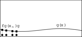
(j)

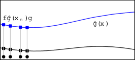
(k)

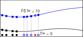
(l)

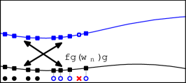
(m)

(n)

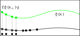
(o)

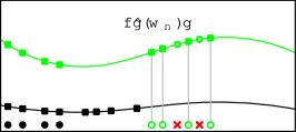
(p)

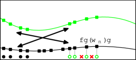
(q)

(r)

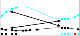
(s)

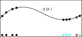
(t)

Figure 2: A cartoon of three exchange sampling transitions. In the first two transitions, the proposals are rejected to demonstrate the expanding Markov state due to retrospective sampling of $g(\boldsymbol{x})$. The third proposal is accepted and the previously-accumulated state is discarded. (a) The observed data, illustrated as  . (b) The initial $g(\boldsymbol{x})$ evaluated at the data, shown as  . (c) The proposed $\hat{g}(\boldsymbol{x})$ evaluated at the data, shown as  . (d) Fantasies are drawn from $\hat{g}(\boldsymbol{x})$, illustrated as  . There is one rejected proposal, shown as  , with the corresponding function value illustrated as  . (e) $g(\boldsymbol{x})$ is evaluated at the fantasies and the two explanations are compared using Equation 4.1. (f) The proposal $\hat{g}(\boldsymbol{x})$ is rejected. The Markov state expands to include the fantasies. (g) A new $\hat{g}(\boldsymbol{x})$, shown in green, is evaluated at the data. (h) Fantasies are drawn from $\hat{g}(\boldsymbol{x})$ (two rejected fantasy proposals). (i) $g(\boldsymbol{x})$ is evaluated at the fantasies and the explanations are compared. (j) The proposal was rejected. The Markov state expands to twelve function evaluations. (k) Skipping the intermediate steps, propose, fantasise, evaluate and compare, using the function shown in cyan. (l) The proposal is accepted and made the new $g(\boldsymbol{x})$. All of the information about the old function is thrown away, but the new $g(\boldsymbol{x})$ must keep information in its conditioning set about the fantasies it generated.

4.1.1 Improving the acceptance rate

For clarity, we introduced the algorithm with ${q(\boldsymbol{\hat{g}}\leftarrow\boldsymbol{g})=p(\boldsymbol{\hat{g}}\,|\,\theta)}$, but this proposal is a poor choice in practice. To achieve a better acceptance rate, it is better to make conservative, perturbative proposals. This can be achieved by introducing a set of $B$ “control points” in $\mathcal{X}$, denoted $\mathcal{C}=\{\boldsymbol{x}_{b}\in\mathcal{X}\}^{B}_{b=1}$. These control points have associated function values, which we denote as ${\mathcal{G}=\{g(\boldsymbol{x}_{b})\}^{B}_{b=1}}$. We assume that $\mathcal{C}$ is a superset of the observed data, i.e., $\mathcal{D}\subseteq\mathcal{C}$. The function values at the control points are explicitly included in the Markov state and all retrospective function draws condition on these points. New discoveries about the function continue to accumulate in the conditioning sets as before. The difference now is that the conditioning sets are initialised with the control points and small, perturbative proposals can be made on the function values at those initial points.

To make this construction explicit, Equation 4.3 is extended to

$$p(\mathcal{G},\boldsymbol{g}_{\backslash\mathcal{C}},\mathcal{D},\hat{\mathcal{G}},\boldsymbol{\hat{g}}_{\backslash\mathcal{C}},\mathcal{W}\,|\,\mathcal{C},\theta,\psi)=\\ \mathcal{GP}(\mathcal{G}\,|\,\mathcal{C},\theta)\;\mathcal{GP}(\boldsymbol{g}_{\backslash\mathcal{C}}\,|\,\mathcal{G},\theta)\,\mathcal{Z}_{\pi}[\boldsymbol{g}]^{-N}\left[\prod^{N}_{n=1}\Phi(g(\boldsymbol{x}_{n}))\;\pi(\boldsymbol{x}_{n}\,|\,\psi)\right]\\ \times q(\hat{\mathcal{G}}\leftarrow\mathcal{G})\;\mathcal{GP}(\boldsymbol{\hat{g}}_{\backslash\mathcal{C}}\,|\,\hat{\mathcal{G}},\theta)\;\mathcal{Z}_{\pi}[\boldsymbol{\hat{g}}]^{-N}\prod^{N}_{n=1}\Phi(\hat{g}(\boldsymbol{w}_{n}))\;\pi(\boldsymbol{w}_{n}\,|\,\psi),$$ (4.5)

where $\hat{\mathcal{G}}$ indicates the proposal of the function values at the control points, i.e. ${\hat{\mathcal{G}}=\{\hat{g}(\boldsymbol{x}_{b})\}^{B}_{b=1}}$, and $\boldsymbol{g}_{\backslash\mathcal{C}}$ denotes the function values, excluding those at $\mathcal{C}$. The proposal density $q(\hat{\mathcal{G}}\leftarrow\mathcal{G})$ can be chosen to take smaller steps than the prior draws of the previous section. With the joint distribution in Equation 4.5, and using the conditional retrospective exchange sampling as before, the acceptance ratio of exchanging the pair $(\mathcal{G},\boldsymbol{g}_{\backslash\mathcal{C}})$ for $(\hat{\mathcal{G}},\boldsymbol{\hat{g}}_{\backslash\mathcal{C}})$ is

$$a_{\textsf{exch-cp}} =\frac{q(\mathcal{G}\leftarrow\hat{\mathcal{G}})\;\mathcal{GP}(\hat{\mathcal{G}}\,|\,\mathcal{C},\theta)}{q(\hat{\mathcal{G}}\leftarrow\mathcal{G})\;\mathcal{GP}(\mathcal{G}\,|\,\mathcal{C},\theta)}\prod^{N}_{n=1}\frac{\Phi(\hat{g}(\boldsymbol{x}_{n}))\;\Phi(g(\boldsymbol{w}_{n}))}{\Phi(g(\boldsymbol{x}_{n}))\;\Phi(\hat{g}(\boldsymbol{w}_{n}))}.$$ (4.6)

Superficially, this might seem similar to the knot-based imputation method of Tokdar (2007). However, whereas Tokdar (2007) uses knots as a finite-dimensional approximation, we use the control points simply to constrain the proposal distribution. The control points only initialise the retrospective sampling procedure. As we enforce a Gaussian process prior on the function values of the control points, the inference procedure still yields the correct posterior distribution on the uncompromised fully-nonparametric Gaussian process density sampler model. The number and locations of the control points are free parameters.

A new function is proposed by first choosing values at the control points close to the existing function. The remainder of the function is drawn from the prior, conditioned on the values at the control points. We always include the locations of the observed data as control points, i.e., $\mathcal{D}\subset\mathcal{C}$. This is not required for the algorithm to be valid, but is convenient as all proposed functions must be evaluated at the data in any case. Taking account of the arbitrary proposal density at the control points, $q(\{\hat{g}(\boldsymbol{x}_{k})\}^{K}_{k=1}\leftarrow\{g(\boldsymbol{x}_{k})\}^{K}_{k=1})$, the exchange sampling acceptance ratio becomes

$$a_{\textsf{exch-control}}=\frac{q(\{g(\boldsymbol{x}_{k})\}^{K}_{k=1}\leftarrow\{\hat{g}(\boldsymbol{x}_{k})\}^{K}_{k=1})\;p(\{\hat{g}(\boldsymbol{x}_{k})\}^{K}_{k=1}\,|\,\theta)}{q(\{\hat{g}(\boldsymbol{x}_{k})\}^{K}_{k=1}\leftarrow\{g(\boldsymbol{x}_{k})\}^{K}_{k=1})\;p(\{g(\boldsymbol{x}_{k})\}^{K}_{k=1}\,|\,\theta)}\\ \times\prod^{N}_{n=1}\frac{\Phi(\hat{g}(\boldsymbol{x}_{n}))\;\Phi(g(\boldsymbol{w}_{n}))}{\Phi(g(\boldsymbol{x}_{n}))\;\Phi(\hat{g}(\boldsymbol{w}_{n}))}.$$ (4.7)

The functions drawn from the Gaussian process must still be evaluated at a larger conditioning set that includes the locations of fantasies. As before, these can be drawn “retrospectively” as needed, but now these Gaussian process samples are conditioned on the values at the control points.

4.1.2 Hyperparameter inference

One of the benefits of the Bayesian approach is the ability to perform hierarchical inference. In this case, it allows us to infer the hyperparameters $\theta$ of the Gaussian process and the hyperparameters $\psi$ of the base density. We augment the exchange sampling algorithm slightly to sample from the posterior on hyperparameters: before proposing a new function $\hat{g}(\boldsymbol{x})$, we propose new hyperparameters $\hat{\theta}$ and $\hat{\psi}$ from a proposal density $q(\hat{\theta},\hat{\psi}\leftarrow\theta,\psi)$. When samples of the new function are drawn, it is done with these proposed hyperparameters. The new joint distribution is

$$p(\boldsymbol{g},\{\boldsymbol{x}_{n}\}^{N}_{n=1},\theta,\psi,\boldsymbol{\hat{g}},\{\boldsymbol{w}_{n}\}^{N}_{n=1},\hat{\theta},\hat{\psi})=\\ p(\theta,\psi)\;p(\boldsymbol{g}\,|\,\theta)\;p(\{\boldsymbol{x}_{n}\}^{N}_{n=1}\,|\,\boldsymbol{g},\psi)\\ \times q(\hat{\theta},\hat{\psi}\leftarrow\theta,\psi)\;p(\boldsymbol{\hat{g}}\,|\,\hat{\theta})\;p(\{\boldsymbol{w}_{n}\}^{N}_{n=1}\,|\,\boldsymbol{\hat{g}},\hat{\psi})$$ (4.8)

where $p(\theta,\psi)$ is an appropriate hyperprior. The proposal is now to exchange the triplets $(\boldsymbol{g},\theta,\psi)$ and $(\boldsymbol{\hat{g}},\hat{\theta},\hat{\psi})$. The acceptance of this swap has Metropolis–Hastings ratio

$$a_{\textsf{exch-hyper}}=\frac{q(\theta,\psi\leftarrow\hat{\theta},\hat{\psi})\;p(\hat{\theta},\hat{\psi})}{q(\hat{\theta},\hat{\psi}\leftarrow\theta,\psi)\;p(\theta,\psi)}\\ \times\prod^{N}_{n=1}\frac{\Phi(\hat{g}(\boldsymbol{x}_{n}))\;\pi(\boldsymbol{x}_{n}\,|\,\hat{\psi})\;\Phi(g(\boldsymbol{w}_{n}))\;\pi(\boldsymbol{w}_{n}\,|\,\psi)}{\Phi(g(\boldsymbol{x}_{n}))\;\pi(\boldsymbol{x}_{n}\,|\,\psi)\;\Phi(\hat{g}(\boldsymbol{w}_{n}))\;\pi(\boldsymbol{w}_{n}\,|\,\hat{\psi})}.$$ (4.9)

This acceptance ratio generalises straightforwardly to the case with control points discussed in Section 4.1.1.

4.1.3 Sampling from the predictive distribution

An important task for density inference is estimation of the predictive density. The predictive distribution arises on data space when the posterior is integrated out. For the GPDS, this density is

$$p(\boldsymbol{x}\,|\,\mathcal{D}) =\int\mathrm{d}\theta\int\mathrm{d}\psi\int\mathrm{d}\boldsymbol{g}\;p(\boldsymbol{x}\,|\,\boldsymbol{g},\theta,\psi)\;p(\boldsymbol{g},\theta,\psi\,|\,\mathcal{D}).$$ (4.10)

The predictive distribution can also be thought of as the distribution on the next datum to arrive, given the $N$ already seen and taking uncertainty into account. In the GPDS, the predictive density in Equation 4.10 is not available analytically. We nevertheless have all the tools in place to generate samples from the predictive distribution. We do this by using the generative procedure of Section 3 to generate additional data after each Metropolis–Hastings step. We use a very similar method to Algorithm 3.1, but initialise the conditioning set using the current state of the Markov chain.

4.2 Sampling over latent histories

An alternative to inference via exchange sampling is to model the latent history of the generative process. By using the GPDS prior to model the data, we are asserting that the data can be explained as the result of Algorithm 3.1. However, we did not observe any of the intermediate states of the rejection sampling algorithm, such as the number and locations of the rejected proposals, and the value of the function sampled from the Gaussian process prior. Nevertheless, Algorithm 3.1 provides a well-defined probabilistic model over both the observed data and this latent state. By modeling this larger joint distribution we can avoid evaluating the intractable normalisation constant that would otherwise appear in the likelihood function.

We model the data ${\mathcal{D}=\{\boldsymbol{x}_{n}\}^{N}_{n=1}}$ as having been generated exactly as in Algorithm 3.1, i.e., run until exactly $N$ proposals were accepted. The state space of the Markov chain on latent histories in the GPDS consists of: 1) the values of the latent function $g(\boldsymbol{x})$ at the data, denoted ${\mathcal{G}_{N}=\{g(\boldsymbol{x}_{n})\}^{N}_{n=1}}$, 2) the number of rejections $M$, 3) the locations of the $M$ rejected proposals, denoted ${\mathcal{M}=\{\boldsymbol{x}_{m}\}^{M}_{m=1}}$, and 4) the values of the latent function $g(\boldsymbol{x})$ at the $M$ rejected proposals, denoted ${\mathcal{G}_{M}=\{g(\boldsymbol{x}_{m})\}^{M}_{m=1}}$. The joint distribution over the data and the ordered history of the GPDS generative procedure, given the hyperparameters, is

$$p(\mathcal{D},\mathcal{G}_{N},\mathcal{M},\mathcal{G}_{M}\,|\,\theta,\psi)=\mathcal{GP}(\mathcal{G}_{N},\mathcal{G}_{M}\,|\,\mathcal{D},\mathcal{M},\theta)\\ \times\left[\prod^{N}_{n=1}\Phi(g(\boldsymbol{x}_{n}))\,\pi(\boldsymbol{x}_{n}\,|\,\psi)\right]\prod^{M}_{n=1}(1-\Phi(g(\boldsymbol{x}_{m})))\,\pi(\boldsymbol{x}_{m}\,|\,\psi).$$ (4.11)

We sample from the posterior distribution over all unknowns, which is proportional to the joint distribution with the observations, $\mathcal{D}$, clamped. The Markov chain algorithm applies three types of update in sequence: 1) modification of the number of rejections $M$, 2) updating of the rejection locations $\mathcal{M}$, and 3) modification of the latent function values $\mathcal{G}_{M}$ and $\mathcal{G}_{N}$. We will maintain an explicit ordering of the latent rejections for reasons of clarity, although this is not necessary due to exchangeability. At any time we could propose a reshuffling of the latent history, subject to it ending in an acceptance, and this proposal would always be accepted, as the two permutations have the same probability under the model.

Inference by Markov chain Monte Carlo of the history of a probabilistic computational procedure has been studied previously. Beskos et al. (2006) sampled from the state of a rejection sampler for diffusions. Murray (2007), who coined the phrase “latent history,” modeled data as having been the result of a Markov chain which had provably mixed via coupling from the past (Propp and Wilson, 1996). Another example is Huber and Wolpert (2009), who model the history of the Matérn Type III process to perform tractable inference. The Church programming language (Goodman et al., 2008) also exploits this idea, by treating probabilistic procedures as first class objects on which inference can be performed.

4.2.1 Modifying the number of latent rejections

We propose a new number of latent rejections $\hat{M}$ by drawing it from a proposal density $q(\hat{M}~{}\leftarrow~{}M)$. If $\hat{M}$ is greater than $M$, we must also propose new rejections to add to the latent state. We take advantage of the exchangeability of the process to generate the new rejections: we imagine these proposals were made after the last observed datum was accepted, and our proposal is to call them rejections and move them before the last datum. If $\hat{M}$ is less than $M$, we do the opposite by proposing to move some rejections to after the last acceptance.

When proposing additional rejections, we must also propose times for them among the current latent history. There are ${\hat{M}+N-1\choose\hat{M}-M}$ such ways to insert these additional rejections into the existing latent history, such that the sampler terminates after the $N$th acceptance. When removing rejections, we must choose which ones to place after the data, and there are ${M\choose M-\hat{M}}$ possible sets. Upon simplification, the proposal ratios for both addition and removal of rejections are identical:

$$\overbrace{\frac{q(M\!\leftarrow\!\hat{M}){\hat{M}+N-1\choose\hat{M}-M}}{q(\hat{M}\!\leftarrow\!M){\hat{M}\choose\hat{M}-M}}}^{\hat{M}>M}=\overbrace{\frac{q(M\!\leftarrow\!\hat{M}){M\choose M-\hat{M}}}{q(\hat{M}\!\leftarrow\!M){M+N-1\choose M-\hat{M}}}}^{\hat{M}<M}=\frac{q(M\!\leftarrow\!\hat{M})M!(\hat{M}\!+\!N\!-\!1)!}{q(\hat{M}\!\leftarrow\!M)\hat{M}!(M\!+\!N\!-\!1)!}.$$

When inserting rejections, we propose the locations of the additional proposals, denoted $\mathcal{M}^{+}$, and the corresponding values of the latent function, denoted $\mathcal{G}^{+}_{M}$. We generate $\mathcal{M}^{+}$ by making $\hat{M}~{}-~{}M$ independent draws from the base density. We draw $\mathcal{G}^{+}_{M}$ jointly from the Gaussian process prior, conditioned on all of the current latent state, i.e., $(\mathcal{M},~{}\mathcal{G}_{M},~{}\mathcal{D},~{}\mathcal{G}_{N})$. The joint probability of this state is

$$p(\mathcal{D},\mathcal{M},\mathcal{M}^{+},\mathcal{G}_{N},\mathcal{G}_{M},\mathcal{G}^{+}_{M}\,|\,\theta,\psi)=\left[\prod_{n=1}^{N}\pi(\boldsymbol{x}_{n}\,|\,\psi)\;\Phi(g(\boldsymbol{x}_{n}))\right]\\ \times\left[\prod_{m=1}^{M}\pi(\boldsymbol{x}_{m}\,|\,\psi)\;(1-\Phi(g(\boldsymbol{x}_{m})))\right]\left[\prod_{m=M+1}^{\hat{M}}\!\!\!\!\pi(\boldsymbol{x}_{m}\,|\,\psi)\right]\\ \times\mathcal{GP}(\mathcal{G}_{M},\mathcal{G}_{N},\mathcal{G}^{+}_{M}\,|\,\mathcal{D},\mathcal{M},\mathcal{M}^{+},\theta).$$ (4.12)

The joint distribution in Equation 4.12 expresses the probability of all the base density draws, the values of the function draws from the Gaussian process, and the acceptance or rejection probabilities of the proposals excluding the newly generated points. When we make an insertion proposal, exchangeability allows us to shuffle the ordering without changing the probability; the only change is that now we must account for labeling the new points as rejections. In the acceptance ratio, all terms except for the “labeling probability” cancel. The reverse proposal is similar, however we denote the removed proposal locations as $\mathcal{M}^{-}$ and the corresponding function values as $\mathcal{G}^{-}_{M}$. The overall acceptance ratios for insertions or removals are

$$a_{\sf{hist-num}}=\begin{cases}\frac{q(M\leftarrow\hat{M})\;M!\;(\hat{M}+N-1)!}{q(\hat{M}\leftarrow M)\;\hat{M}!\;(M+N-1)!}\prod_{g\in\mathcal{G}^{+}_{M}}(1-\Phi(g))&\text{if $\hat{M}>M$}\\ \quad\\ \frac{q(M\leftarrow\hat{M})\;M!\;(\hat{M}+N-1)!}{q(\hat{M}\leftarrow M)\;\hat{M}!\;(M+N-1)!}\prod_{g\in\mathcal{G}^{-}_{M}}(1-\Phi(g))^{-1}&\text{if $\hat{M}<M$}.\end{cases}$$ (4.13)

A simple and convenient way of implementing this procedure is to make limited proposals that either insert or delete only one latent rejection at a time. We define a function ${\zeta(M,N):\mathbb{N}\times\mathbb{N}^{+}\to(0,1]}$ and propose inserting a new latent rejection with probability $\zeta$. Otherwise, with with probability $1-\zeta$, we propose removing a rejection. We must, of course, enforce ${\zeta(0,N)=1}$. With these limited proposals, the first case of Equation 4.13 (proposing one new latent rejection, i.e., ${\hat{M}=M+1}$) can be written as

$$a_{\sf{hist-ins}} =\frac{(1-\zeta(M+1,N))\;(M+N)\;(1-\Phi(g(\boldsymbol{x}^{+})))}{\zeta(M,N)\;(M+1)},$$ (4.14)

where $\boldsymbol{x}^{+}$ is the proposed rejection location. The location $\boldsymbol{x}^{+}$ is drawn from the base density $\pi(\boldsymbol{x}\,|\,\psi)$. In the second case, if there is at least one latent rejection in the current history (${M>0}$), then the deletion of a single rejection is proposed, i.e., ${\hat{M}=M-1}$. This deletion proposal has Metropolis–Hastings acceptance ratio

$$a_{\sf{hist-del}} =\frac{\zeta(M-1,N)\;M}{(1-\zeta(M,N))\;(M+N-1)\;(1-\Phi(g(\boldsymbol{x}^{-})))},$$ (4.15)

where $\boldsymbol{x}^{-}$ is the location of the proposed removal. The rejection to remove is chosen uniformly from among the $M$ currently in the history.

4.2.2 Modifying latent rejection locations

Given the number of latent rejections $M$ and the current latent function, we would like to sample from the locations of the rejections. Given the latent function, the locations of the rejections are independent. We make perturbative proposals of new locations, conditionally sample the function from the Gaussian process and then accept or reject with Metropolis–Hastings.

The current locations of the rejections are denoted $\mathcal{M}$ and we draw a proposal $\hat{\mathcal{M}}$ from a proposal distribution $q(\hat{\mathcal{M}}\leftarrow\mathcal{M})$. The values of the latent function at $\mathcal{M}$ are denoted $\mathcal{G}_{M}$ and we sample the function at $\hat{\mathcal{M}}$ jointly from the Gaussian process prior given $\mathcal{D}$, $\mathcal{G}_{N}$, $\mathcal{M}$, and $\mathcal{G}_{M}$. The Metropolis–Hastings acceptance ratio of this proposal is

$$a_{\sf{hist-locs}} =\frac{q(\mathcal{M}\leftarrow\hat{\mathcal{M}})}{q(\hat{\mathcal{M}}\leftarrow\mathcal{M})}\prod^{M}_{m=1}\frac{\pi(\boldsymbol{\hat{x}}_{m}\,|\,\psi)\;(1-\Phi(\hat{g}(\boldsymbol{x}_{m})))}{\pi(\boldsymbol{x}_{m}\,|\,\psi)\;(1-\Phi(g(\boldsymbol{x}_{m})))}.$$ (4.16)

4.2.3 Modifying the latent function values

Conditioned on the number and location of the latent rejections, we must also sample from the latent function at both the data and rejection locations. The conditional joint posterior distribution is

$$p(\mathcal{G}_{N},\mathcal{G}_{M}\,|\,\mathcal{M},\mathcal{D},\theta)=\mathcal{GP}(\mathcal{G}_{N},\mathcal{G}_{M}\,|\,\mathcal{D},\mathcal{M},\theta)\\ \times\left[\prod^{N}_{n=1}\Phi(g(\boldsymbol{x}_{n}))\right]\left[\prod^{M}_{m=1}\left(1-\Phi(g(\boldsymbol{x}_{m}))\right)\right].$$ (4.17)

This joint distribution is easily sampled using Hybrid (Hamiltonian) Monte Carlo (Duane et al., 1987). For numerical reasons we suggest performing gradient calculations in the “whitened” space resulting from applying the inverse Cholesky decomposition of the covariance matrix to the function values.

Algorithm 4.2 implements the latent history algorithm in pseudocode, with the simple $q(\hat{M}\leftarrow M)$ that proposes increasing or decreasing the number of latent rejections $M$ by one.

4.2.4 Hyperparameter inference

Given a sample from the posterior on the latent history, we can also perform a Metropolis–Hastings step in the space of hyperparameters. As in Section 4.1.2, we have hyperparameters $\theta$ for the Gaussian process and $\psi$ for the base density, with joint prior density $p(\theta,\psi)$. We introduce the proposal density $q(\hat{\theta},~{}\hat{\psi}~{}\leftarrow~{}\theta,~{}\psi)$ to make proposals $\hat{\theta}$ and $\hat{\psi}$. The acceptance ratio for a Metropolis–Hastings step in the posterior of the hyperparameters, given the latent history, is

$$a_{\sf{hist-hp}}=\frac{q(\theta,\psi\!\leftarrow\!\hat{\theta},\hat{\psi})\;p(\hat{\theta},\hat{\psi})\;\mathcal{N}(\{\mathcal{G}_{M},\mathcal{G}_{N}\}\,|\,\mathcal{M},\mathcal{D},\hat{\theta})}{q(\hat{\theta},\hat{\psi}\!\leftarrow\!\theta,\psi)\;p(\theta,\psi)\;\mathcal{N}(\{\mathcal{G}_{M},\mathcal{G}_{N}\}\,|\,\mathcal{M},\mathcal{D},\theta)}\\ \times\left[\prod_{m=1}^{M}\frac{\pi(\boldsymbol{x}_{m}\,|\,\hat{\psi})}{\pi(\boldsymbol{x}_{m}\,|\,\psi)}\right]\left[\prod_{n=1}^{N}\frac{\pi(\boldsymbol{x}_{n}\,|\,\hat{\psi})}{\pi(\boldsymbol{x}_{n}\,|\,\psi)}\right].$$ (4.18)

1:

2:Number of MCMC iterations $R$

3:Observed data $\mathcal{D}=\{\boldsymbol{x}_{n}\}^{N}_{n=1}$

4:Gaussian process covariance function $C(\boldsymbol{x},\boldsymbol{x}^{\prime};\theta)$

5:Base density $\pi(\boldsymbol{x}\,|\,\psi)$

6:Location proposal density $q(\boldsymbol{\hat{x}}_{m}\leftarrow\boldsymbol{x}_{m})$

7:Insert proposal probability function $\zeta(M,N)$

8:

9:$R$ samples of the latent history $\{\mathcal{M}^{(r)},\mathcal{G}^{(r)}_{N},\mathcal{G}^{(r)}_{M}\}^{R}_{r=1}$

10:$\mathcal{M}\leftarrow\emptyset$, $\mathcal{G}_{M}\leftarrow\emptyset$ $\triangleright$ Start out with no latent rejections.

11:$\mathcal{G}_{N}\sim\mathcal{GP}(g\,|\,\mathcal{D},\theta)$ $\triangleright$ Initialise the function at the data.

12:for $r\leftarrow 1\ldots R$ do $\triangleright$ Take $R$ MCMC steps on the latent history.

13:     $u_{\zeta}\sim\textsf{Un}(0,1)$ $\triangleright$ Draw a uniform random variate on $(0,1)$.

14:     if $u_{\zeta}<\zeta(|\mathcal{M}|,N)$ then $\triangleright$ Decide whether to insert or delete.

15:         $\boldsymbol{x}^{+}\sim\pi(\boldsymbol{x}\,|\,\psi_{\pi})$ $\triangleright$ Draw a proposed rejection location.

16:         $g(\boldsymbol{x}^{+})\sim\mathcal{GP}(g\,|\,\boldsymbol{x}^{+},\mathcal{D},\mathcal{M},\mathcal{G}_{M},\mathcal{G}_{N},\theta)$ $\triangleright$ Draw the proposed function value.

17:         $a_{\sf{hist-ins}}\leftarrow\displaystyle\frac{(1-\zeta(|\mathcal{M}|+1,N))\;(|\mathcal{M}|+N)\;(1-\Phi(g(\boldsymbol{x}^{+})))}{\zeta(|\mathcal{M}|,N)\;(|\mathcal{M}|+1)}$ $\triangleright$ Acceptance ratio.

18:         $u_{\sf{ins}}\sim\textsf{Un}(0,1)$ $\triangleright$ Draw a uniform random variate on $(0,1)$.

19:         if $u_{\sf{ins}}<a_{\sf{hist-ins}}$ then $\triangleright$ Metropolis–Hastings acceptance rule.

20:              $\mathcal{M}\leftarrow\mathcal{M}\cup\boldsymbol{x}^{+}$, $\mathcal{G}_{M}\leftarrow\mathcal{G}_{M}\cup g(\boldsymbol{x}^{+})$ $\triangleright$ Add this new rejection.

21:         end if

22:     else if $|\mathcal{M}|>0$ then

23:         $m\sim\lceil\textsf{Un}(0,|\mathcal{M}|)\rceil$ $\triangleright$ Select one of the $M$ rejections at random.

24:         $a_{\sf{hist-del}}=\displaystyle\frac{\zeta(|\mathcal{M}|-1,N)\;|\mathcal{M}|}{(1-\zeta(|\mathcal{M}|,N))\;(|\mathcal{M}|+N-1)\;(1-\Phi(g(\boldsymbol{x}_{m})))}$ $\triangleright$ Acceptance ratio.

25:         $u_{\sf{del}}\sim\textsf{Un}(0,1)$ $\triangleright$ Draw a uniform random variate on $(0,1)$.

26:         if $u_{\sf{del}}<a_{\sf{hist-del}}$ then $\triangleright$ Metropolis–Hastings acceptance rule.

27:              $\mathcal{M}\leftarrow\mathcal{M}\backslash\boldsymbol{x}_{m}$, $\mathcal{G}_{M}\leftarrow\mathcal{G}_{M}\backslash g(\boldsymbol{x}_{m})$ $\triangleright$ Remove the $m$th rejection.

28:         end if

29:     end if

30:     for $m\leftarrow 1\ldots M$ do $\triangleright$ Loop over the latent rejections.

31:         $\boldsymbol{\hat{x}}_{m}\sim q(\boldsymbol{\hat{x}}_{m}\leftarrow\boldsymbol{x}_{m})$ $\triangleright$ Propose a new location.

32:         $g(\boldsymbol{\hat{x}}_{m})\sim\mathcal{GP}(g\,|\,\boldsymbol{\hat{x}}_{m},\mathcal{D},\mathcal{M},\mathcal{G}_{N},\mathcal{G}_{M},\theta)$ $\triangleright$ Draw a function value from the GP.

33:         $a_{\sf{hist-loc}}=\displaystyle\frac{q(\boldsymbol{x}_{m}\leftarrow\boldsymbol{\hat{x}}_{m})\;\pi(\boldsymbol{\hat{x}}_{m})\;(1-\Phi(g(\boldsymbol{\hat{x}}_{m})))}{q(\boldsymbol{\hat{x}}_{m}\leftarrow\boldsymbol{x}_{m})\;\pi(\boldsymbol{x}_{m})\;(1-\Phi(g(\boldsymbol{x}_{m})))}$ $\triangleright$ Acceptance ratio.

34:         $u_{\sf{loc}}\sim\textsf{Un}(0,1)$ $\triangleright$ Draw a uniform random variate from $(0,1)$.

35:         if $u_{\sf{loc}}<a_{\sf{hist-loc}}$ then $\triangleright$ Metropolis–Hastings acceptance rule.

36:              $\boldsymbol{x}_{m}\leftarrow\boldsymbol{\hat{x}}_{m}$, $g(\boldsymbol{x}_{m})\leftarrow g(\boldsymbol{\hat{x}}_{m})$ $\triangleright$ Update the rejection.

37:         end if

38:     end for

39:     $\mathcal{G}_{N}$,$\mathcal{G}_{M}\sim\textsf{HMC}(\mathcal{G}_{N},\mathcal{G}_{M}\,|\,\mathcal{D},\mathcal{M},\theta)$ $\triangleright$ Update function via Hybrid Monte Carlo.

40:     $\mathcal{M}^{(r)}\leftarrow\mathcal{M}$, $\mathcal{G}^{(r)}_{N}\leftarrow\mathcal{G}_{N}$, $\mathcal{G}^{(r)}_{M}\leftarrow\mathcal{G}_{M}$ $\triangleright$ Store the current version of the history.

41:end for

42:return $\{\mathcal{M}^{(r)},\mathcal{G}^{(r)}_{N},\mathcal{G}^{(r)}_{M}\}^{R}_{r=1}$

Algorithm 4.2 Simulate $R$ steps of a Markov chain on the latent history

4.2.5 Generating predictive samples

As with the exchange sampling approach in Section 4.1.3, it is possible to generate samples from the predictive density. As each state in the Markov chain of the latent history inference is a rejection sampler state, it is simply a matter of continuing the rejection procedure forward to produce a new sample.

4.3 Calculating the predictive density

We have shown that each inference method can yield predictive samples, but it is also natural to require that a density model provide an estimate of the normalized predictive density itself. We use the method of Chib and Jeliazkov (2001), which considers Metropolis–Hastings moves between a pair $\boldsymbol{x}$ and $\boldsymbol{x}^{\prime}$. Using the base density $\pi(\boldsymbol{x}\,|\,\psi)$ as the proposal density, the detailed balance condition for Metropolis–Hastings gives the identity

$$p(\boldsymbol{x},\boldsymbol{g},\theta,\psi)\;\pi(\boldsymbol{x}^{\prime}\,|\,\psi)\;\min\left(1,\frac{\Phi(g(\boldsymbol{x}^{\prime}))}{\Phi(g(\boldsymbol{x}))}\right)=\\ p(\boldsymbol{x}^{\prime},\boldsymbol{g},\theta,\psi)\;\pi(\boldsymbol{x}\,|\,\psi)\;\min\left(1,\frac{\Phi(g(\boldsymbol{x}))}{\Phi(g(\boldsymbol{x}^{\prime}))}\right).$$ (4.19)

We integrate both sides of this identity over $x^{\prime}$ and take the expectation of each side under the posterior over the function $\boldsymbol{g}$ and the hyperparameters $\theta$ and $\psi$:

$$\int\!\!\!\mathrm{d}\theta\!\!\int\!\!\!\mathrm{d}\psi\!\int\!\!\!\mathrm{d}\boldsymbol{g}\;p(\boldsymbol{g},\theta,\psi\,|\,\mathcal{D})\int\!\!\mathrm{d}x^{\prime}\;p(\boldsymbol{x}\,|\,\boldsymbol{g},\theta,\psi)\;\pi(\boldsymbol{x}^{\prime}\,|\,\psi)\;\min\left(1,\frac{\Phi(g(\boldsymbol{x}^{\prime}))}{\Phi(g(\boldsymbol{x}))}\right)=\\ \int\!\!\!\mathrm{d}\theta\!\int\!\!\!\mathrm{d}\psi\!\int\!\!\!\mathrm{d}\boldsymbol{g}\;p(\boldsymbol{g},\theta,\psi\,|\,\mathcal{D})\int\!\!\mathrm{d}x^{\prime}\;p(\boldsymbol{x}^{\prime}\,|\,\boldsymbol{g},\theta,\psi)\;\pi(\boldsymbol{x}\,|\,\psi)\;\min\left(1,\frac{\Phi(g(\boldsymbol{x}))}{\Phi(g(\boldsymbol{x}^{\prime}))}\right).$$

We observe that

$$p(\boldsymbol{g},\theta,\psi\,|\,\mathcal{D})\;p(\boldsymbol{x}\,|\,\boldsymbol{g},\theta,\psi)=p(\boldsymbol{x},\boldsymbol{g},\theta,\psi\,|\,\mathcal{D})=p(\boldsymbol{x}\,|\,\mathcal{D})\;p(\boldsymbol{g},\theta,\psi\,|\,x,\mathcal{D})$$

and so we may find the predictive density via

$$p(\boldsymbol{x}\,|\,\mathcal{D}) =\frac{\int\!\mathrm{d}\theta\!\int\!\mathrm{d}\psi\!\int\!\mathrm{d}\boldsymbol{g}\!\int\!\mathrm{d}x^{\prime}\;p(\theta,\psi,\boldsymbol{g},x^{\prime}\,|\,\mathcal{D})\;\pi(\boldsymbol{x}\,|\,\psi)\;\min\left(1,\frac{\Phi(g(\boldsymbol{x}))}{\Phi(g(\boldsymbol{x}^{\prime}))}\right)}{\int\!\mathrm{d}\theta\!\int\!\mathrm{d}\psi\!\int\!\mathrm{d}\boldsymbol{g}\!\int\!\mathrm{d}x^{\prime}\;p(\theta,\psi,\boldsymbol{g}\,|\,x,\mathcal{D})\;\pi(\boldsymbol{x}^{\prime}\,|\,\psi)\;\min\left(1,\frac{\Phi(g(\boldsymbol{x}^{\prime}))}{\Phi(g(\boldsymbol{x}))}\right)}$$ (4.20)

Both the numerator and the denominator in Equation 4.20 are expectations. The top is an expectation under the posterior and the bottom is an expectation under the posterior where the data has been augmented with $x$:

$$p(\boldsymbol{x}\,|\,\mathcal{D}) =\frac{\mathbb{E}_{p(\boldsymbol{g},\theta,\psi,x^{\prime}|\mathcal{D})}\left[\pi(\boldsymbol{x}\,|\,\psi)\;\min\left(1,\frac{\Phi(g(\boldsymbol{x}))}{\Phi(g(\boldsymbol{x}^{\prime}))}\right)\right]}{\mathbb{E}_{p(\boldsymbol{g},\theta,\psi|\mathcal{D},x)}\left[\mathbb{E}_{\pi(\boldsymbol{x}^{\prime}\,|\,\psi)}\left[\min\left(1,\frac{\Phi(g(\boldsymbol{x}^{\prime}))}{\Phi(g(\boldsymbol{x}))}\right)\right]\right]}.$$ (4.21)

The numerator can be estimated directly as part of the MCMC inference. After each Markov step, generate a predictive sample $x^{\prime}$ and record the transition probabilities. The denominator requires a Markov chain to be run with a data set augmented by the predictive location $x$. At each step in the Markov chain, a sample $x^{\prime}$ is generated from the base density and the transition probabilities are evaluated.

5 Examples

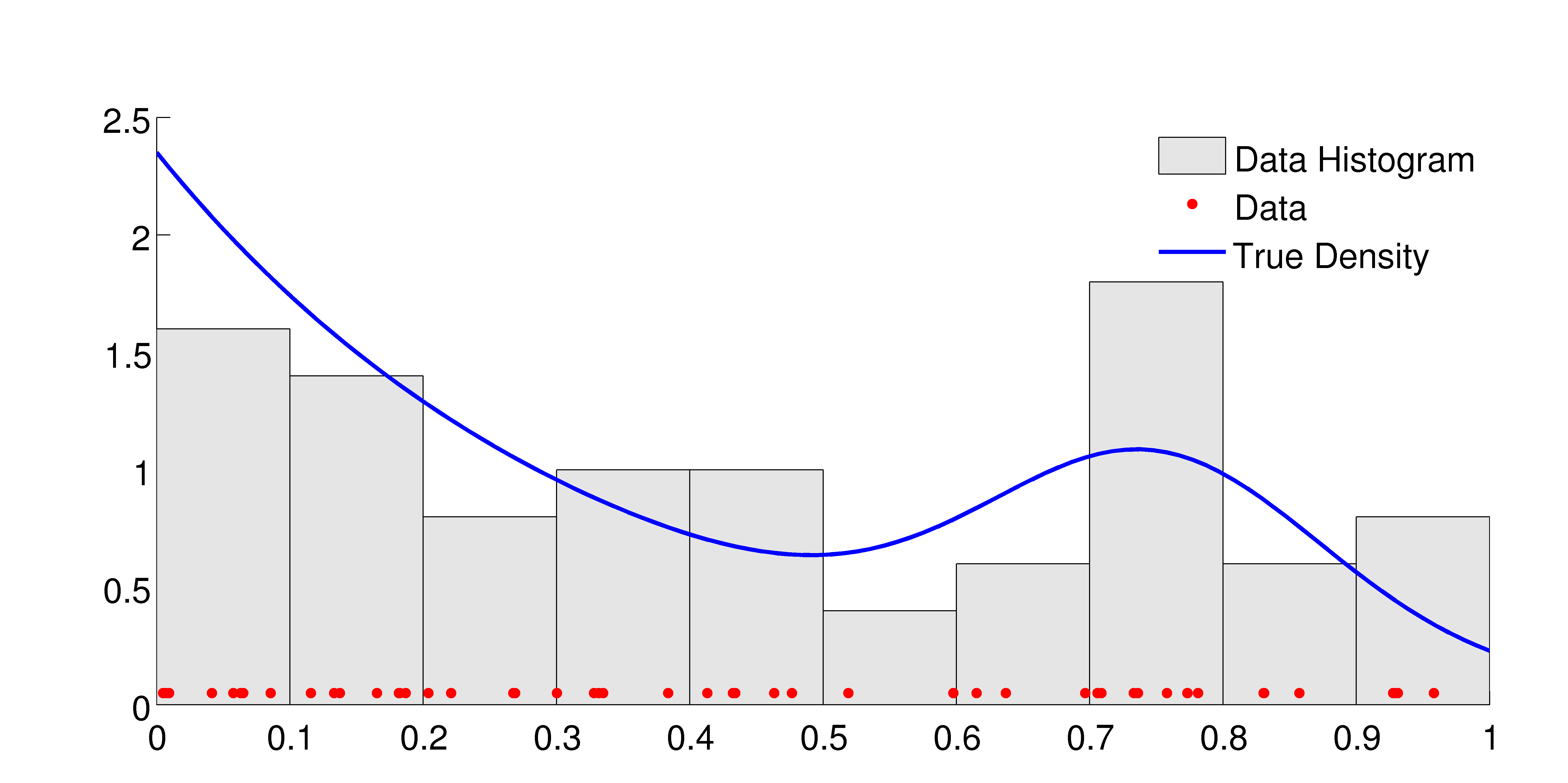
(a)

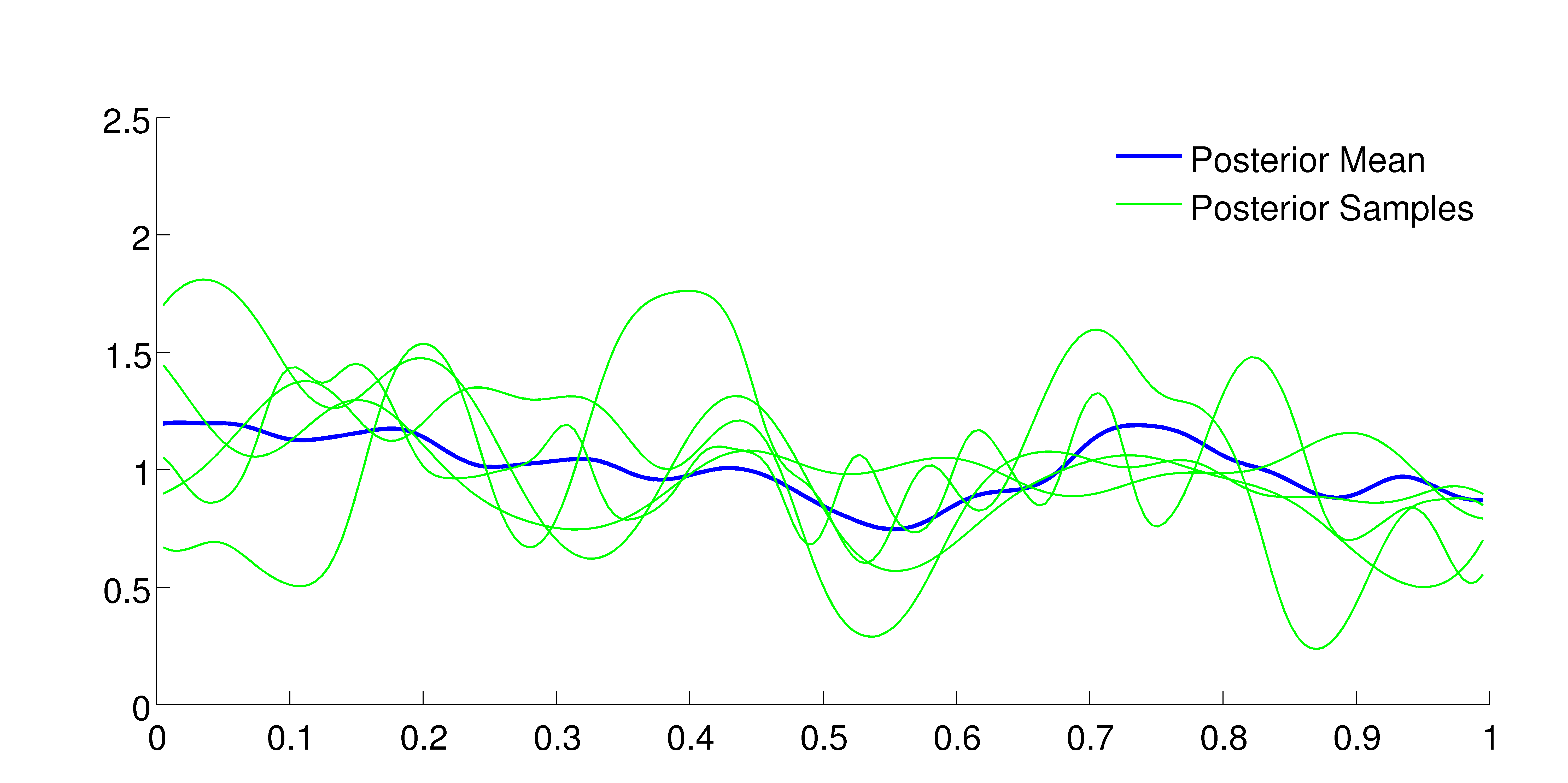
(b)

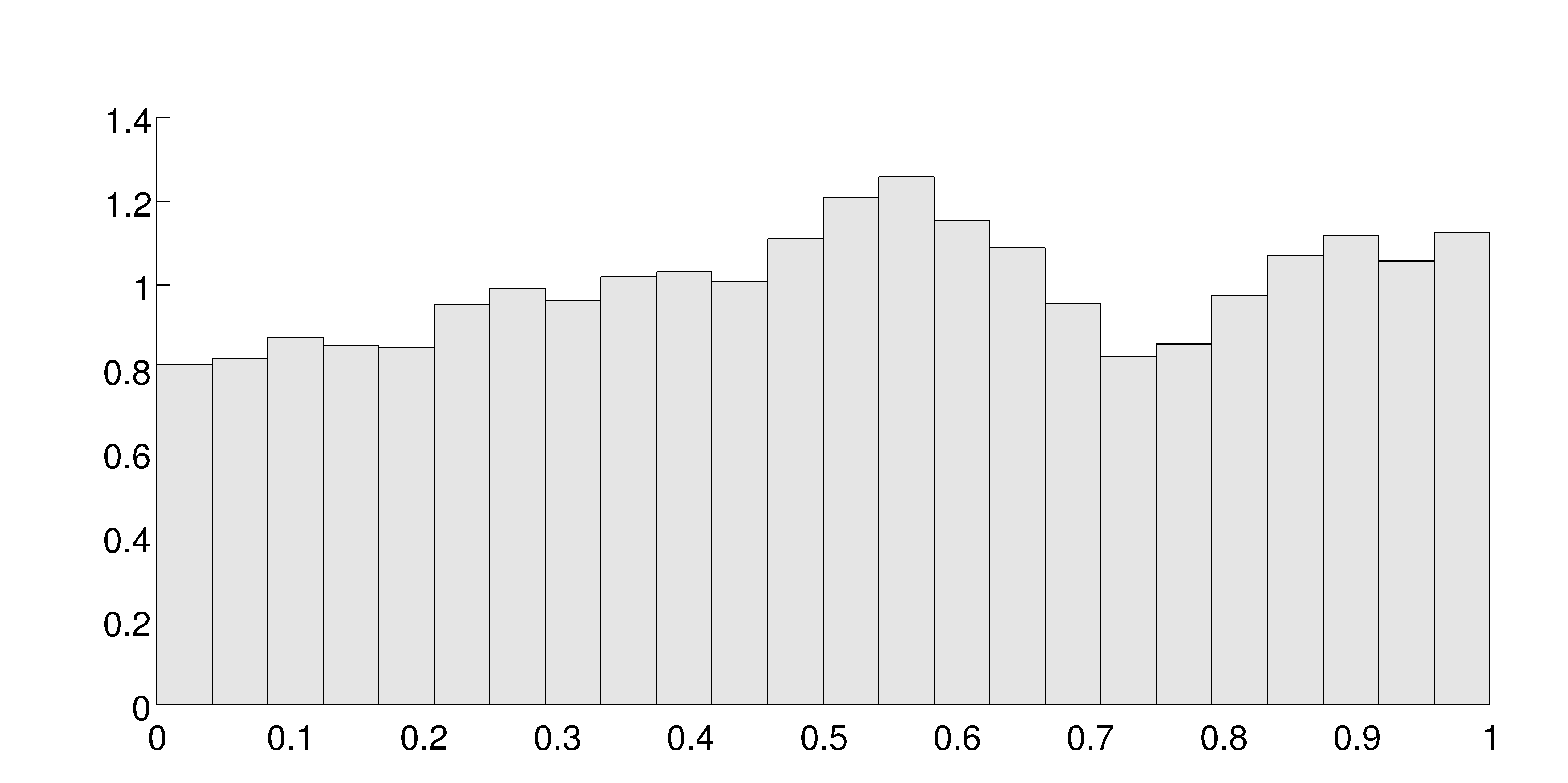
(c)

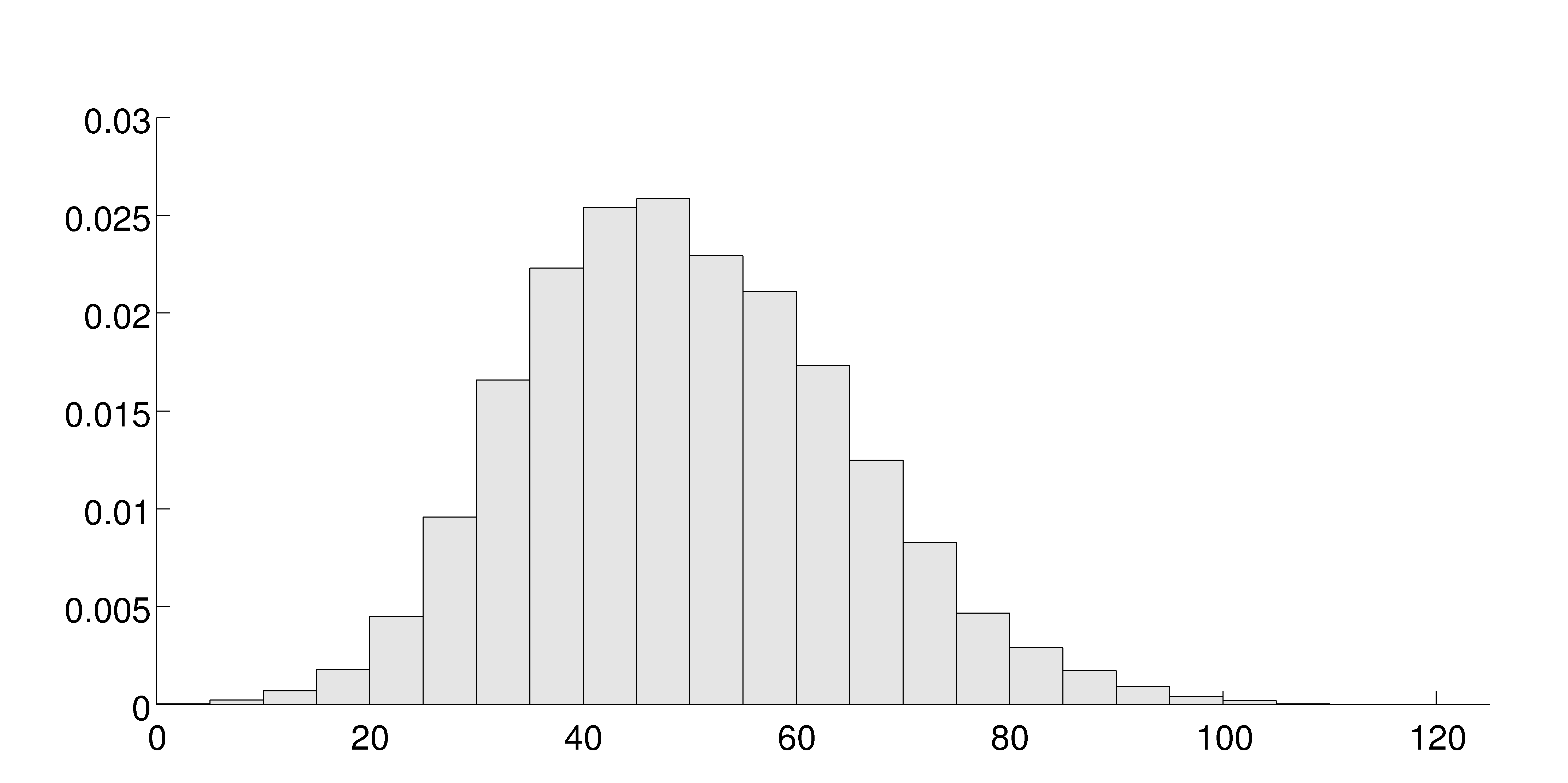
(d)

Figure 3: Bounded one-dimensional example

5.1 One-Dimensional Bounded Density

We examined the GPDS on the one-dimensional problem studied by Lenk (1991) and Tokdar (2007). It is a mixture of an exponential and normal density on $[0,1]$:

$$f_{1}(x) =\frac{3}{4}\cdot 3\exp\{-3x\}+\frac{1}{4}\cdot\left(\frac{\pi}{32}\right)^{-\frac{1}{2}}\exp\Bigg{\{}-32\left(x-\frac{3}{4}\right)^{2}\Bigg{\}}.$$ (5.1)

50 independent observations were drawn from this density and latent history inference with the GPDS was applied to it. Figure 3a shows a histogram of the observations and the true density. The base density for the GPDS was chosen to be the uniform distribution on $(0,1)$. The covariance function used was the stationary squared exponential:

$$C(x,x^{\prime}) =\alpha^{2}\exp\left\{-\frac{1}{2}\left(\frac{x-x^{\prime}}{\ell}\right)^{2}\right\}$$ (5.2)

and the parameters $\alpha$ and $\ell$ were included in MCMC sampling for both the GPDS and the logistic Gaussian process. The priors used for the Gaussian process hyperparameters were

$$\ln\alpha \sim\mathcal{N}(\mu=1,\,\sigma=0.5)$$ (5.3)

$$\ln\ell \sim\mathcal{N}(\mu=0.05,\,\sigma=0.5).$$ (5.4)

The Markov chain was simulated for 50,000 iterations, with the first 10,000 discarded as burn-in. Figure 3b shows the predictive density from the MCMC run, along with several posterior samples. Figure 3c shows a histogram of the locations of the rejections in the latent history inference, and Figure 3d is a histogram of the number of rejections in samples from the latent history.

5.2 Two-Dimensional Unbounded Density

We generated 200 independent observations from a two-dimensional location mixture of Gaussians, where the means are drawn uniformly from a ring of radius $3/2$, centred at the origin. The Gaussians have a variance of $1/16$ so that the data density is

$$f_{2}(x_{1},x_{2}) =\frac{4}{9\pi}\int_{-\pi}^{\pi}\!\!\!\!\mathrm{d}\vartheta\;\mathcal{N}(x_{1}\,;\,3/2\cos\vartheta,\sigma=1/4)\mathcal{N}(x_{2}\,;\,3/2\sin\vartheta,\sigma=1/4).$$

We used the two-dimensional isotropic variant of the covariance function given by Equation 5.2 and used a Gaussian distribution for the base density, inferring the mean and covariance as in Section 4.2.4. We simulated the Markov chain for 50,000 iterations, discarding 10,000 as burn-in. The true density and the observed data are shown in Figure 4a, while the posterior predictive density and a posterior sample of rejection location are shown in Figure 4b. As expected, the rejections tend to accumulate in the center of the ring, where the base density places mass but the predictive density should be low.

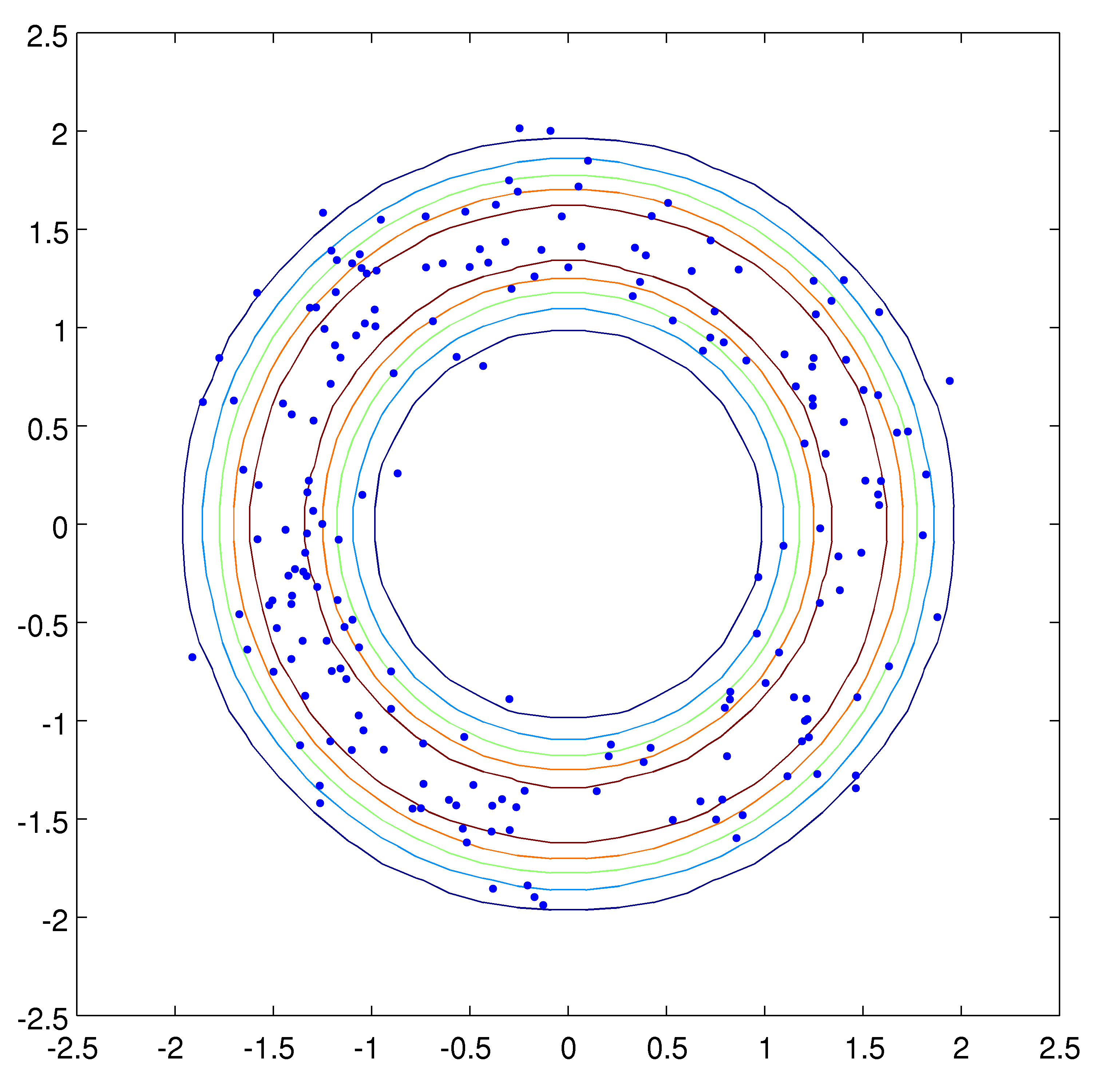
(a)

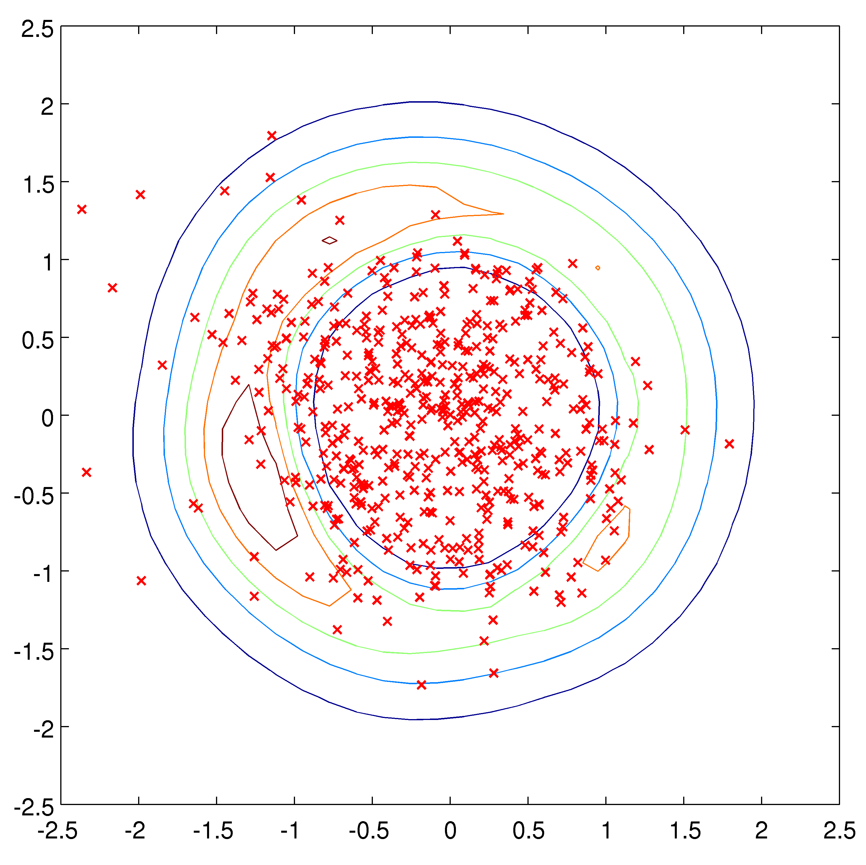
(b)

Figure 4: Synthetic ring mixture example

6 Discussion

6.1 Computational issues

Computation with a Gaussian process is expensive. If the GP is realised on $R$ points, the space complexity of storing the covariance (Gram) matrix is $O(R^{2})$ and the time complexity of decomposing (or inverting) the matrix is $O(R^{3})$. The time cost of this decomposition will be the asymptotically-dominating factor when performing GPDS inference using either exchange sampling or the latent history method.

6.2 Comparing exchange sampling and latent history inference

Modeling of probability densities is fundamentally different from regression. In regression and classification, one conditions on having seen data in the input space when performing inference and prediction. In these cases, it is necessary only to model the function at places where data have been observed, or at predictive query locations. In density modeling, however, the places with low density are just as important to the model as those with high density. Unfortunately, it is unlikely to have observed data in regions with low density, so a representation of the function only at locations where there are data is not adequate for the inference we wish to perform. One might think of defining a density as analogous to putting up a tent: pinning the canvas down with pegs (or stakes) is just as important as putting up poles. In exchange sampling, the “pegs” are inferred implicitly as rejections along the way to generating fantasy data. At each exchange sampling step, a new tent is constructed — complete with its own pegs — and asked to explain the data. In the latent history model, however, the tent is modified one piece at a time: pegs and poles are inserted, removed, and adjusted gradually to explain the data.

It is possible also to see that the latent history model is likely to require fewer samples from the Gaussian process as it proceeds. Consider the Gaussian process density sampler: when the latent history method is at equilibrium, its state will have some typical number of latent rejections $M$. This is about the same number of rejections as would be expected to occur during an exchange sampling fantasy. However, to find the acceptance ratio in exchange sampling it is also necessary to evaluate against the observed data after fantasising. This means that the Gaussian process in exchange sampling requires at least $2N+M$ evaluations to make a Metropolis–Hastings move, while the latent history method requires only $N+M$. This does not even consider the expansion of state that occurs when exchange sampling rejects a proposal, and additional fantasy data are incorporated into the Markov state. As the time complexity of computation in the Gaussian process grows cubically in the number of data, exchange sampling can become rapidly more expensive.

Another reason that the latent history method is preferable to exchange sampling is that it requires less bookkeeping about the function $g(\boldsymbol{x})$. The state of the exchange sampling Markov chain is the uncountably-infinite object $g(\boldsymbol{x})$. The innovation of the method is that through retrospective sampling we are able to make Metropolis–Hastings moves with only a finite number of computations. This retrospective sampling, however, means that information discovered about a particular $g(\boldsymbol{x})$ must be retained for as long as that function is relevant to the current Markov state. In contrast, the state of the Markov chain when performing latent history inference only includes $g(\boldsymbol{x})$ at the latent rejections or thinned events. That is, rather than an uncountably-infinite object $g(\boldsymbol{x})$, the Gaussian process in the latent history model conditions on a finite set of points in the input space. This means that the values of the function do not need to be kept in memory, except for at the data and at the locations of the rejections or thinned events. This contrast can also be seen in the difference between the joint distributions that describe the two inference methods for the Gaussian process density sampler. In exchange sampling, when writing Equation 4.3, we use $\boldsymbol{g}$ to denote $g(\boldsymbol{x})$ as an infinite vector. When writing the posterior distribution on the latent history, however, we do not need to denote an infinite function. Equation 4.11 only defines a distribution on the function values at the data and the latent rejections.

Finally, while the latent history method enables efficient Hamiltonian Monte Carlo sampling of the latent function values, it is not clear how to combine HMC with exchange sampling.

6.3 Restricting the function space

With both the exchange sampling and latent history methods, incorporating fewer latent rejections (“tent pegs”) into the Gaussian process results in improved efficiency. For a given $g(\boldsymbol{x})$, the expected number of rejections is $N(\mathcal{Z}_{\pi}[g]^{-1}-1)$. This expression is derived from the observation that $\pi(\boldsymbol{x}\,|\,\psi)$ provides an upper bound on the function $\Phi(g(\boldsymbol{x}))\,\pi(\boldsymbol{x}\,|\,\psi)$ and the ratio of acceptances to rejections is determined by the proportion of the mass of $\pi(\boldsymbol{x}\,|\,\psi)$ contained by $\Phi(g(\boldsymbol{x}))\,\pi(\boldsymbol{x}\,|\,\psi)$. One problem with inference is that there are many functions $g(\boldsymbol{x})$ that can explain the data equivalently, as $\Phi(g(\boldsymbol{x}))\,\pi(\boldsymbol{x}\,|\,\psi)$ is unnormalised. Many of these $g(\boldsymbol{x})$ will cause $\Phi(g(\boldsymbol{x}))$ to be close to zero, resulting in many rejections. The Gaussian process prior might only provide weak regularisation to prevent this.

One way to improve this situation is to require that the function $g(\boldsymbol{x})$ be pinned to zero for some $\boldsymbol{x}_{0}$. This prevents $\Phi(g(\boldsymbol{x}))\,\pi(\boldsymbol{x}\,|\,\psi)$ from being small everywhere and reduces the redundancy in the prior that occurs due to normalisation. We use the base density $\pi(\boldsymbol{x}\,|\,\psi)$ as a prior on $\boldsymbol{x}_{0}$ and treat it as a hyperparameter for the Gaussian process. We can then use the inference methods of Sections 4.1.2 and 4.2.4 to infer an appropriate $\boldsymbol{x}_{0}$.

6.4 The logistic Gaussian process

The Gaussian process is an appealing prior on functions due to the ability to specify the smoothness and differentiability properties of sample realizations via a covariance function, without choosing an explicit set of basis functions. This flexibility and intuition has led to interest in applying Gaussian processes to density modeling via the logistic Gaussian process introduced by Leonard (1978) and further developed by Lenk (1988, 1991). If $g(\boldsymbol{x})$ is a random function drawn from a Gaussian process, then the logistic GP arrives at a density $f(\boldsymbol{x})$ on a closed interval $\mathcal{I}$ via

$$f(\boldsymbol{x}) =\frac{e^{g(\boldsymbol{x})}}{\int_{\mathcal{I}}e^{g(\boldsymbol{x})}}$$ (6.1)

for $\boldsymbol{x}\in\mathcal{I}$. On a bounded interval and with minor constraints on the covariance function, the integral in the denominator exists and the density is well-defined Tokdar (2007). The distribution on densities is closed under Bayesian updating. As in Equation 2.1, however, it is generally impossible to integrate an infinite-dimensional random function and so likelihood-based calculations are intractable. The GP-based prior we have presented in this paper allows exact inference computation despite this intractability by constructing a generative model, but no such method is known for the logistic Gaussian process.

In order to perform inference with the logistic Gaussian process, several finite-dimensional approximations have been introduced. Lenk (1991, 2003) proposes an approximation of the logistic GP by a truncated Karhunen–Loève expansion evaluated on a grid. Tokdar (2007) uses a finite-dimensional approximation to the logistic Gaussian process by parameterizing the function values on a grid and then imputing other values from the conditional mean. The normalisation constant is estimated via a numeric method, e.g.,the trapezoidal rule or Simpson’s rule.

The approach of expanding the density as a finite Fourier series, as described by Lenk (2003), is appealing in a single dimension as one can parameterize the function in terms of coefficients with independent Gaussian priors. The variances of these priors arise directly from the Gaussian process covariance function. As noted by Lenk (2003), however, the number of Fourier coefficients required grows exponentially with dimension. Finding higher-dimensional bases that are rich enough to express interesting structure while also allowing efficient computation is considered an open problem.

The imputation method of Tokdar (2007) extends to the multivariate case more straightforwardly. While a lattice does not scale well to many dimensions, the imputation approximation does not necessarily require a grid. Tokdar (2007) proposes a method of inferring appropriate knot locations and explores this on a two-dimensional test problem using reversible jump Markov chain Monte Carlo (Green, 1995). This has a similar motivation to the model presented in this paper: adapt the parameterization of the Gaussian process as the data demands. The GPDS achieves this via a fully-nonparametric generative model, Tokdar (2007) specifies a finite-dimensional surrogate model with the dimensionality selected as a part of inference. Additionally, it is unclear in Tokdar (2007) how the normalization constant is to be effectively estimated when the knots are irregularly arranged. It is suggested to perform imputation to a grid from the known knots, but this reintroduces some aspects of the problems of lattices in high dimensions. In contrast, the GPDS inference discussed in the present paper explicitly avoids these problems by performing computation without evaluating $\mathcal{Z}_{\pi}[\boldsymbol{g}]$.

References

- Beskos et al. [2006] A. Beskos, O. Papaspiliopoulos, G. O. Roberts, and P. Fearnhead. Exact and computationally efficient likelihood-based estimation for discretely observed diffusion processes (with discussion). Journal of the Royal Statistical Society: Series B, 68:333–382, 2006.
- Chib and Jeliazkov [2001] S. Chib and I. Jeliazkov. Marginal likelihood from the Metropolis–Hastings output. Journal of the American Statistical Association, 96(453):270–281, 2001.
- Csató [2002] L. Csató. Gaussian processes - iterative sparse approximations. PhD thesis, Aston University, Birmingham, UK, March 2002.
- DiMatteo et al. [2001] I. DiMatteo, C. R. Genovese, and R. E. Kass. Bayesian curve-fitting with free-knot splines. Biometrika, 88(4):1055–1071, 2001.
- Duane et al. [1987] S. Duane, A. D. Kennedy, B. J. Pendleton, and D. Roweth. Hybrid Monte Carlo. Physics Letters B, 195(2):216–222, 1987.
- Escobar and West [1995] M. D. Escobar and M. West. Bayesian density estimation and inference using mixtures. Journal of the American Statistical Association, 90(430):577–588, June 1995.
- Ferguson [1973] T. S. Ferguson. A Bayesian analysis of some nonparametric problems. The Annals of Statistics, 1(2):209–230, 1973.
- Goodman et al. [2008] N. D. Goodman, V. K. Mansinghka, D. M. Roy, K. Bonawitz, and J. B. Tenenbaum. Church: a language for generative models. In Proceedings of the 24th Annual Conference on Uncertainty in Artificial Intelligence, 2008.
- Green [1995] P. J. Green. Reversible jump Markov chain Monte Carlo computation and Bayesian model selection. Biometrika, 82:711–732, 1995.
- Huber and Wolpert [2009] M. L. Huber and R. L. Wolpert. Likelihood-based inference for Matérn type III repulsive point processes. Advances in Applied Probability, 41(4), 2009. In press.
- Ishwaran and James [2001] H. Ishwaran and L. F. James. Gibbs sampling methods for stick-breaking priors. Journal of the American Statistical Association, 96(453):161–173, March 2001.
- Lavine [1992] M. Lavine. Some aspects of Pólya tree distributions for statistical modelling. Annals of Statistics, 20(3):1222–1235, 1992.
- Lavine [1994] M. Lavine. More aspects of Pólya tree distributions for statistical modelling. Annals of Statistics, 22(3):1161–1175, 1994.
- Lenk [1988] P. J. Lenk. The logistic normal distribution for Bayesian, nonparametric, predictive densities. Journal of the American Statistical Association, 83(402):509–516, 1988.
- Lenk [1991] P. J. Lenk. Towards a practicable Bayesian nonparametric density estimator. Biometrika, 78(3):531–543, 1991.
- Lenk [2003] P. J. Lenk. Bayesian semiparametric density estimation and model verification using a logistic-Gaussian process. Journal of Computational and Graphical Statistics, 12(3):548–565, 2003.
- Leonard [1978] T. Leonard. Density estimation, stochastic processes and prior information. Journal of the Royal Statistical Society, Series B, 40(2):113–146, 1978.
- Lo [1984] A. Y. Lo. On a class of Bayesian nonparametric estimates: I. density estimates. The Annals of Statistics, 12(1):351–357, March 1984.
- MacKay [1992] D. J. C. MacKay. Bayesian interpolation. Neural Computation, 4(3):415–447, 1992.
- Møller et al. [2006] J. Møller, A. N. Pettit, R. Reeves, and K. K. Bethelsen. An efficient Markov chain Monte Carlo method for distributions with intractable normalising constants. Biometrika, 93(2):451–458, 2006.
- Murray [2007] I. Murray. Advances in Markov chain Monte Carlo methods. PhD thesis, Gatsby Computational Neuroscience Unit, University College London, London, 2007.
- Murray et al. [2006] I. Murray, Z. Ghahramani, and D. J. C. MacKay. MCMC for doubly-intractable distributions. In Proceedings of the 22nd Annual Conference on Uncertainty in Artificial Intelligence (UAI), pages 359–366, 2006.
- Neal [2001] R. M. Neal. Defining priors for distributions using Dirichlet diffusion trees. Technical Report 0104, Department of Statistics, University of Toronto, 2001.
- Neal [2003] R. M. Neal. Density modeling and clustering using Dirichlet diffusion trees. In Bayesian Statistics 7, pages 619–629, 2003.
- O’Hagan [1978] A. O’Hagan. Curve fitting and optimal design for prediction. Journal of the Royal Statistical Society, Series B, 40:1–42, 1978.
- Papaspiliopoulos and Roberts [2008] O. Papaspiliopoulos and G. O. Roberts. Retrospective Markov chain Monte Carlo methods for Dirichlet process hierarchical models. Biometrika, 95(1):169–186, 2008.
- Pitman and Yor [1997] J. Pitman and M. Yor. The two-parameter Poisson-Dirichlet distribution derived from a stable subordinator. Annals of Probability, 25:855–900, 1997.
- Propp and Wilson [1996] J. G. Propp and D. B. Wilson. Exact sampling with coupled Markov chains and applications to statistical mechanics. Random Structures and Algorithms, 9(1&2):223–252, 1996.
- Rasmussen and Williams [2006] C. E. Rasmussen and C. K. I. Williams. Gaussian Processes for Machine Learning. MIT Press, Cambridge, MA, 2006.
- Thorburn [1986] D. Thorburn. A Bayesian approach to density estimation. Biometrika, 73(1):65–75, 1986.
- Tokdar [2007] S. T. Tokdar. Towards a faster implementation of density estimation with logistic Gaussian process priors. Journal of Computational and Graphical Statistics, 16(2):1–23, 2007.
- Tokdar and Ghosh [2007] S. T. Tokdar and J. K. Ghosh. Posterior consistency of logistic Gaussian process priors in density estimation. Journal of Statistical Planning and Inference, 137:34–42, 2007.