Abstract

We construct a holographic dark energy model in a braneworld setup that gravity is induced on the brane embedded in a bulk with Gauss-Bonnet curvature term. We include possible modification of the induced gravity and its coupling with a canonical scalar field on the brane. Through a perturbational approach to calculate the effective gravitation constant on the brane, we examine the outcome of this model as a candidate for holographic dark energy.
PACS: 04.50.-h,  98.80.-k, 95.36.+x
Key Words: Braneworld Cosmology, Dark Energy, Scalar-Tensor Theories, Modified Gravity

1 Introduction

It is observationally confirmed from supernovae distance-redshift data, the microwave background radiation, the large scale structure, weak lensing and baryon oscillations that the current expansion of the universe is accelerating [1]. There are several approaches to explain this late-time accelerated expansion of the universe. One of these approaches, is to introduce some sort of unknown energy component ( the dark energy) which has negative pressure (See [2] and references therein). The simplest candidate in this respect is a cosmological constant in the framework of the general relativity. However, huge amount of fine-tuning, no dynamical behavior and also unknown origin of emergence make its unfavorable [3]. Another alternative is a dynamical dark energy: the cosmological constant puzzles may be better interpreted by assuming that the vacuum energy is canceled to exactly zero by some unknown mechanism and introducing a dark energy component with a dynamically variable equation of state [2]. Nevertheless, the main problem with the dark energy is that its nature and cosmological origin are still obscure at present. Other alternatives to accommodate present accelerated expansion of the universe are modified gravity [4] and some braneworld scenarios such as the Dvali-Gabadadze-Porrati (DGP) scenario [5]. Here, we are interested in to probe the nature of dark energy in the context of holographic dark energy models. The idea of holographic dark energy comes from quantum gravity considerations [6]. This model proposes that if $\rho_{\Lambda}$ is the quantum zero-point energy density caused by a short distance cut-off, the total energy in a region of size $L$ should not exceed the mass of a black hole of the same size. The holographic dark energy density corresponds to a dynamical cosmological constant and in this respect, the standard General Relativity should be modified by some gravitational terms which became relevant at present accelerating universe. Modified gravity provides the natural gravitational alternative for dark energy. Moreover, modified gravity presents a natural unification of the early time inflation and late-time acceleration due to different role of gravitational terms relevant at small and at large curvature [4,7]. Also modified gravity may naturally describe the transition from non-phantom phase to phantom one without necessity to introduce the exotic matter. $f(R)$ gravity is one successful attempt in this direction. Another theory proposed as gravitational dark energy is the scalar-Gauss-Bonnet gravity which is closely related with low-order string effective action [8]. The possibility to extend such consideration to third order (curvature cubic) terms in low-energy string effective action exists too [9]. Moreover, one can develop the reconstruction method for such theories [10]. It has been demonstrated that some scalar-Gauss-Bonnet gravities may be compatible with the known classical history of the universe expansion [7].

In this paper we propose a unified $f(R)$-Gauss-Bonnet gravity with non-minimal coupling of the scalar field to $f(R)$. We proceed a holographic dark energy approach to examine cosmological dynamics in this setup and we show that this model accounts for phantom-like behavior. This model presents a smooth crossing of the phantom divide line by its equation of state parameter and this crossing occurs in the same way as is supported observationally, that is, from above -1 to its below.

2 The Setup

The action of our modified GBIG model contains the Gauss-Bonnet term in the bulk and modified induced gravity term on the brane where a scalar field non-minimally coupled to induced gravity is present on the brane

$$S=\frac{1}{2\kappa_{5}^{2}}\int d^{5}x\sqrt{-g^{(5)}}\bigg{\{}R^{(5)}-2\Lambda_{5}+\beta\bigg{[}R^{(5)2}-4R_{ab}^{(5)}R^{(5)ab}+R_{abcd}^{(5)}R^{(5)abcd}\bigg{]}\bigg{\}}$$

$$+\int_{brane}d^{4}x\sqrt{-q}\bigg{[}M_{5}^{3}K^{\pm}+\frac{M_{4}^{2}}{2}\,\alpha(\varphi)f(R)-\lambda-[\bigtriangledown\phi]^{2}-2V(\phi)+L_{m}\bigg{]}\ ,$$ (1)

where $\beta$($\geq 0$) is the GB coupling constant,  $\kappa_{5}^{2}$ is the five dimensional gravitational constant,  $\lambda$ is the brane tension, $\Lambda_{5}$ is the bulk cosmological constant and  $\overline{K}$  is the trace of the mean extrinsic curvature of the brane.

To obtain cosmological dynamics in this setup, we use the following line-element

$$ds^{2}=q_{\mu\nu}dx^{\mu}dx^{\nu}+b^{2}(y,t)dy^{2}=-n^{2}(y,t)dt^{2}+a^{2}(y,t)\gamma_{ij}dx^{i}dx^{j}+b^{2}(y,t)dy^{2}\,,$$ (2)

where $\gamma_{ij}$ is a maximally symmetric 3-dimensional metric defined as $\gamma_{ij}=\delta_{ij}+k\frac{x_{i}x_{j}}{1-kr^{2}}$ and $k=-1,0,1$ parameterizes the spatial curvature. The generalized cosmological dynamics of this setup is given by the following Friedmann equation ( see [11] for details)

$$\bigg{[}1+\frac{8}{3}\beta\bigg{(}H^{2}+\frac{\Phi}{2}+\frac{K}{a^{2}}\bigg{)}\bigg{]}^{2}\bigg{(}H^{2}-\Phi+\frac{K}{a^{2}}\bigg{)}=\Bigg{\{}r\alpha(\varphi)\bigg{[}\bigg{(}H^{2}+\frac{K}{a^{2}}\bigg{)}f^{\prime}(R)\bigg{]}$$

$$-\frac{\kappa_{5}^{2}}{6}\bigg{[}\rho_{m}+\rho_{\varphi}+\lambda+\frac{M_{4}^{2}}{2}\,\alpha(\varphi)\bigg{(}Rf^{\prime}(R)-f(R)-6H\dot{R}f^{\prime\prime}(R)\bigg{)}\bigg{]}\Bigg{\}}^{2}\ ,$$ (3)

where a dash denotes $\frac{d}{dR}$ and a dot marks $\frac{d}{dt}$. The energy-density corresponding to the non-minimally coupled scalar field is as follows

$$\rho_{\varphi}=\bigg{[}\frac{1}{2}\dot{\phi}^{2}+n^{2}V(\varphi)-6f(R)\frac{d\alpha(\varphi)}{d\varphi}H\dot{\varphi}\bigg{]}_{y=0},$$ (4)

where $y$ is the coordinate of the fifth dimension and the brane is located at $y=0$. To proceed further, we set $n^{2}(y,t)|_{y=0}=1$. Now we solve analytically the friedmann equation (3). It is convenient to introduce the dimensionless variables ( see for instance [12])

$$\bar{H}=\frac{8}{3}\frac{\beta}{r\alpha(\varphi)f(R)}H=2\frac{\Omega_{\beta}\sqrt{\Omega_{r}}}{\alpha(\varphi)f(R)}E(z)\,,$$ (5)

$$\bar{\rho}=\frac{32}{27}\frac{\kappa_{5}^{2}\beta^{2}}{r^{3}\alpha^{3}(\varphi)f^{3}(R)}\Big{(}\rho_{m}+\alpha(\varphi)\rho_{\varphi}+\rho_{c}\Big{)}=4\frac{\Omega_{r}\Omega_{\beta}^{2}}{\alpha^{3}(\varphi)f^{3}(R)}\Big{[}\Omega_{\varphi}+\alpha(\varphi)\Omega_{c}+\Omega_{m}(1+z)^{3}\Big{]}\,,$$ (6)

and

$$b=\frac{8}{3}\frac{\beta}{r^{2}\alpha^{2}(\varphi)f^{2}(R)}=4\frac{\Omega_{\beta}\Omega_{r}}{\alpha^{2}(\varphi)f^{2}(R)}\,,$$ (7)

where $r\equiv\frac{\kappa^{2}_{5}}{2\kappa^{2}_{4}}$ is the DGP crossover scale and by definition

$$E(z)\equiv\frac{H}{H_{0}}\,,\,\Omega_{m}\equiv\frac{\kappa_{4}^{2}\rho_{m0}}{3H_{0}^{2}}\,,\,\,\Omega_{\varphi}\equiv\frac{\kappa_{4}^{2}\rho_{\varphi}}{3H_{0}^{2}}\,,\,\,\Omega_{r}\equiv\frac{1}{4r^{2}H_{0}^{2}}\,,\,\,\Omega_{\beta}\equiv\frac{8}{3}\beta H_{0}^{2}\,,\,\Omega_{c}\equiv\frac{\kappa_{4}^{2}\rho_{c}}{3H_{0}^{2}}\,,$$ (8)

where

$$\rho_{c}\equiv\frac{M_{4}^{2}}{2}\bigg{(}Rf^{\prime}(R)-f(R)-6H\dot{R}f^{\prime\prime}(R)\bigg{)}.$$

The Friedmann equation (3) now takes the following compact form

$$\bar{H}^{3}+\bar{H}^{2}+b\bar{H}-\bar{\rho}=0.$$ (9)

The number of real roots of this equation is determined by the sign of the discriminant function N defined as [13]

$$N=Q^{3}+R^{2}$$ (10)

where

$$Q\equiv\frac{1}{3}(b-\frac{1}{3})$$ (11)

$$R\equiv\frac{1}{6}b+\frac{1}{2}\bar{\rho}-\frac{1}{27}\,\,.$$ (12)

If $N>0$, then there is a unique real solution. If $N<0$, there are $3$ real solutions. Finally, if $N=0$, all roots are real and at least two are equal. In which follows, we consider the case with $N>0$ and in this case the unique real solution is given as follows [12,13]

$$\bar{H}=\frac{1}{3}\Bigg{[}2\sqrt{1-3b}\,\cosh(\frac{\eta}{3})-1\Bigg{]}$$ (13)

where

$$\cosh(\eta)=\frac{R}{\sqrt{-Q}}\,\,,\quad\quad\sinh(\eta)=\sqrt{\frac{Q^{3}+R^{2}}{-Q^{3}}}\,\,.$$ (14)

Therefore, we achieve the following solution for the Friedmann equation (3)

$$H=\frac{r\alpha(\varphi)f(R)}{8\beta}\Bigg{[}2\sqrt{1-3b}\,\cosh(\frac{\eta}{3})-1\Bigg{]}.$$ (15)

After obtaining a solution of the Friedmann equation, in the next section we try to provide the basis of a holographic dark energy in this setup.

3 Effective Gravitational Constant

Now we derive the gravitational constant within a perturbation theory to construct our holographic dark energy scenario. Firstly, we analyze the weak field limit of the model presented in the previous section within the slow time-variation approximation and at small scales with respect to the horizon s size. It is convenient to use the longitudinal gauge metric written directly in terms of $\zeta=\log a$

$$ds^{2}=e^{2\zeta}\bigg{[}-(1+2\Psi)\frac{d\zeta^{2}}{a^{2}H^{2}}+(1-2\Upsilon)dx_{i}dx^{i}\bigg{]}$$ (16)

The field $\Psi$ is the Newtonian potential and $\Upsilon$ is the leading-order, spatial post-Newtonian correction which will permit us to calculate the stress-anisotropy. For the longitudinal post-Newtonian limit to be satisfied, we require $\Delta\Upsilon>>a^{2}H^{2}\times(\Upsilon,\dot{\Upsilon},\ddot{\Upsilon})$ and similarly for other gradient terms [14]. For a plane wave perturbation with wavelength $\bar{\lambda}$ , we see that $H^{2}\Upsilon$ is much smaller than $\Delta\Upsilon$ when $\bar{\lambda}<<\frac{1}{H}$ . The requirement that $\dot{\Upsilon}$ is also negligible implies the condition

$$\frac{d\log\Upsilon}{d\zeta}<<\frac{1}{(\bar{\lambda}H)^{2}}\,,$$ (17)

which holds if the condition $\bar{\lambda}<<\frac{1}{H}$ is satisfied for perturbation growth. This argument can be applied for $\ddot{\Upsilon}$,  $\Upsilon$ and $\delta\varphi$. Now using the metric (16), we can rewrite the $(\zeta\zeta)$ and $(ij)$ components of the gravitational field equations and the scalar field equation as follows [14]

$$\frac{3}{2}\,a^{2}H^{2}\delta\Omega_{m}=A\Delta\Upsilon+B\frac{\Delta\delta\varphi}{\dot{\varphi}}$$ (18)

$$A\Delta\Psi=C\Delta\Upsilon+D\frac{\Delta\delta\varphi}{\dot{\varphi}}$$ (19)

$$B\Delta\Psi=D\Delta\Upsilon-E\frac{\Delta\delta\varphi}{\dot{\varphi}}$$ (20)

where $H$ is given by (15) and we have defined the following quantities

$$A=1+\frac{4H^{2}\beta\dot{\varphi}^{2}}{3},$$ (21)

$$B=-\frac{24H^{2}\beta\dot{\varphi}^{2}}{3}+\frac{1}{2}\sqrt{\frac{8}{3}}H^{2}\beta\dot{\varphi}^{3}$$ (22)

$$C=1-\frac{4H^{2}\beta\dot{\varphi}^{2}}{3},$$ (23)

$$D=-\frac{24H^{2}\beta\dot{\varphi}^{2}}{3}\Big{(}\dot{a}+a\frac{\dot{H}}{H}+\frac{\ddot{\varphi}}{\dot{\varphi}}\Big{)},$$ (24)

$$E=\frac{1}{2}\Bigg{(}\dot{\varphi}^{2}-\frac{24H^{2}\beta\dot{\varphi}^{2}}{3}\Big{[}1+2\dot{a}+2a\frac{\dot{H}}{H}\Big{]}+2\sqrt{\frac{8}{3}}H^{2}\beta\dot{\varphi}^{3}\Big{[}1+\dot{a}+a\frac{H}{H}+\frac{\ddot{\varphi}}{\dot{\varphi}}\Big{]}\Bigg{)}.\\$$ (25)

We also include the $(0j)$ component of the gravitation field equations in the same limit

$$\frac{3}{2}\,a^{2}H^{2}\theta\,\Omega_{m}=(B-A)\Delta\Psi+F\frac{\Delta\delta\varphi}{\dot{\varphi}}-A\Delta\dot{\Upsilon}-B\frac{\Delta\dot{\delta\varphi}}{\dot{\varphi}}.$$ (26)

The energy-momentum conservation equations are [14]

$$\dot{\delta}=-\theta$$ (27)

and

$$\dot{\theta}+\theta+(\dot{a}+a\frac{\dot{H}}{H})\theta=-\frac{\Delta\Psi}{a^{2}H^{2}}$$ (28)

where $\delta\equiv\delta\rho/\rho$ is the matter density contrast and $\theta$ is the divergence of the matter peculiar velocity field. Finally, Poisson s equation in this setup is as follows

$$\Delta\Psi=\frac{3G_{eff}}{2G}\,a^{2}H^{2}\delta\Omega_{m}$$ (29)

where $G_{eff}$, the effective gravitational constant, is

$$G_{eff}=G\frac{D^{2}+CE}{A^{2}E+2ABD-B^{2}C}\,.$$ (30)

This equation ( which its derivation can be obtained in [14] with more details) is the basis of our forthcoming arguments. After calculation of the effective gravitational constant, in the next section we construct a holographic dark energy model in the normal branch of this DGP-inspired modified GBIG scenario. We note that since the normal DGP branch is ghost-free and cosmologically stable, there is no ghost instability in our modified GBIG scenario too.

4 Holographic Dark Energy in Modified GBIG Scenario

4.1 General Formalism

To study holographic dark energy model in the modified GBIG scenario, we first present a brief overview of the holographic dark energy model [6]. It is well-known that the mass of a spherical and uncharged D-dimensional black hole is related to its Schwarzschild radius by [15]

$$M_{BH}=r_{s}^{D-3}\Big{(}\sqrt{\pi}M_{D}\Big{)}^{D-3}M_{D}\frac{D-2}{8\Gamma\Big{(}\frac{D-1}{2}\Big{)}}$$ (31)

where the D-dimensional Planck mass, $M_{D}$, is related to the D-dimensional gravitational constant $G_{D}$ and the usual 4-dimensional Planck mass through $M_{D}=G_{D}^{-\frac{1}{D-2}}$ and $M_{p}^{2}=M_{D}^{D-2}V_{D-4}$ with $V_{D-4}$ the volume of the extra-dimensional space. If $\rho_{\Lambda D}$ is the bulk vacuum energy, then application of the holographic dark energy proposal in the bulk gives

$$\rho_{\Lambda D}{\cal{V}}(S^{D-2})\leq r_{D-3}\Big{(}\sqrt{\pi}M_{D}\Big{)}^{D-3}M_{D}\frac{D-2}{8\Gamma\Big{(}\frac{D-1}{2}\Big{)}}$$ (32)

where ${\cal{V}}(S^{D-2})$ is the volume of the maximal hypersphere in a D-dimensional spacetime given by ${\cal{V}}(S^{D-2})=A_{D}r^{D-1}$. $A_{D}$ is defined as

$$A_{D}=\frac{\pi^{\frac{D-1}{2}}}{\Big{(}\frac{D-1}{2}\Big{)}!}$$

$$A_{D}=\frac{\Big{(}\frac{D-2}{2}\Big{)}!}{(D-1)!}2^{D-1}\pi^{\frac{D-2}{2}}$$

for $D-1$ being even or odd respectively. By saturating inequality (27), introducing $L$ as a suitable large distance ( IR cutoff) and $c^{2}$ as a numerical factor, the corresponding vacuum energy as a holographic dark energy is given by [15]

$$\rho_{\Lambda D}=c^{2}\Big{(}\sqrt{\pi}M_{D}\Big{)}^{D-3}M_{D}A_{D}^{-1}\frac{D-2}{8\Gamma\Big{(}\frac{D-1}{2}\Big{)}}L^{-2}.$$ (33)

Using this expression, one can calculate the corresponding pressure via continuity equation and then the equation of state parameter of the holographic dark energy defined as $\omega_{\Lambda}=\frac{\rho_{\Lambda}}{p_{\Lambda}}$ can be obtained directly.

Now we use this formalism in our GBIG setup. There are alternative possibilities to choose $L$ ( see [15]). Here and in our forthcoming arguments we choose the IR cut-off,  $L$  , to be the crossover scale $r$ which is related to the present Hubble radius via $r=1.26H_{0}^{-1}$ ( see for instance the paper by Lue in Ref. [5] and [17]) where $H$ is given by (15). In this case the effective holographic dark energy density is defined as follows

$$\rho_{eff}=\frac{3H^{2}}{8\pi G_{eff}}$$ (34)

where $H$ and $G_{eff}$ are given by (15) and (30) respectively. So we find

$$\rho_{eff}=\frac{3H^{2}}{8\pi G}\Big{(}\frac{A^{2}E+2ABD-B^{2}C}{D^{2}+CE}\Big{)}.$$ (35)

Using the conservation equation

$$\dot{\rho}_{eff}+3H(\rho_{eff}+p_{eff})=0,$$ (36)

we can deduce

$$p_{eff}=H(D^{2}+CE)^{-2}\bigg{[}(2D\dot{D}+\dot{C}E+C\dot{E})(A^{2}E+2ABD-B^{2}C)-(D^{2}+CE)(2A\dot{A}E+A^{2}\dot{E}$$

$$+2\dot{A}BD+2A\dot{B}D+2AB\dot{D}-2B\dot{B}C-B^{2}C)\bigg{]}-\Big{(}\frac{2\dot{H}+3H^{2}}{8\pi G}\Big{)}\Big{(}\frac{A^{2}E+2ABD-B^{2}C}{D^{2}+CE}\Big{)}.$$ (37)

Hence, the equation of state parameter of the model is given as follows

$$\omega_{eff}=\frac{1}{3H}\frac{(2D\dot{D}+\dot{C}E+C\dot{E})(A^{2}E+2ABD-B^{2}C)-(D^{2}+CE)(2A\dot{A}E+A^{2}\dot{E}+2\dot{A}BD+2A\dot{B}D+2AB\dot{D}-2B\dot{B}C-B^{2}C)}{(A^{2}E+2ABD-B^{2}C)(D^{2}+CE)}-\frac{2\dot{H}+3H^{2}}{3H^{2}}.$$ (38)

Now to proceed further, we should specify the form of $f(R)$. In which follows we present a relatively general example by adopting the Hu-Sawicki model.

4.2 An Example

As an example, we consider the following observationally suitable form of $f(R)$ ( the Hu-Sawicki model [16])

$$f(R)=R-R_{c}\frac{\vartheta(R/R_{c})^{m}}{1+(R/R_{c})^{m}},$$ (39)

where for an spatially flat FRW type universe,

$$R=-6(\dot{H}+2H^{2})$$ (40)

and both $\vartheta$ and $R_{c}$ are free positive parameters. We also adopt the ansatz with $a=a_{0}t^{\nu}$ and $\varphi=\varphi_{0}t^{-\mu}$ (with $\nu$ and $\mu$ positive constants) and $\alpha(\varphi)=\frac{1}{2}(1-\xi\varphi^{2})$ with $\xi$ a positive non-minimal coupling. We set $V(\varphi)=V_{0}\varphi^{2}$ and we translate all of our cosmological dynamics equations in terms of the redshift using the relation between $a$ and $z$ as $1+z=\frac{a_{0}}{a}$. One can use these ansatz in the Friedmann, Klein-Gordon and the conservation equations to find constraints on the values of $\nu$ and $\mu$ ( and also $\xi$) to have an accelerating phase of expansion at late-time ( to see a typical analysis in this direction see [17]). Based on such an analysis, in which follows we set $\nu=1.2$ and $\mu=0.5$. The value adopted for $\nu$ gives a late-time accelerating universe. Then we perform some numerical analysis of the model parameter space. We set $\xi=0.15$ which is close to the conformal coupling. The reason for adopting such a value of $\xi$ is motivated from constraint on $\xi$ from recent observations [18]. For our numerical purposes we have set $V_{0}=1$ and $\beta=0.33$. Figure $1$ shows the behavior of the effective energy density, $\rho_{eff}$, versus the redshift. We see that the effective energy density grows with time and always $\rho_{eff}>0$. This is a typical behavior of phantom-like dark energy density. Figure $2$ shows the behavior of $1+\omega_{eff}$ versus the redshift. With the choice of the model parameters as we have adopted here, the universe enters the phantom phase at $z\simeq 0.25$ close to the observationally supported value.

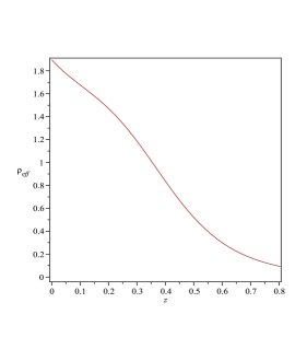
Figure 1: Variation of the effective dark energy density versus the redshift.

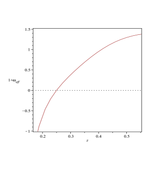
Figure 2: Variation of $1+\omega_{eff}$ versus the redshift.

The deceleration parameter defined as

$$q=-\Big{(}\frac{\dot{H}}{H^{2}}+1\Big{)},$$ (41)

in our setup takes the following form

$$q=-\frac{8\beta\big{(}\dot{f}(R)\alpha(\varphi)+\dot{\alpha}(\varphi)f(R)\big{)}}{rf^{2}(R)\alpha^{2}(\varphi)}\Bigg{[}2\sqrt{1-3b}\,\cosh(\frac{\eta}{3})-1\Bigg{]}^{-1}-\frac{8\beta}{rf(R)\alpha(\varphi)}\Bigg{[}2\sqrt{1-3b}\,\cosh{\frac{\eta}{3}}-1\Bigg{]}^{-2}\Bigg{\{}\frac{-3\dot{b}}{\sqrt{1-3b}}\cosh{\frac{\eta}{3}}+\frac{2}{3}\sqrt{1-3b}\dot{\eta}\sinh{\frac{\eta}{3}}-1\Bigg{\}}-1$$ (42)

Figure $3$ shows the behavior of $q$ versus $z$. In this model, the universe has entered an accelerating phase in the past at $z\simeq 0.84$.

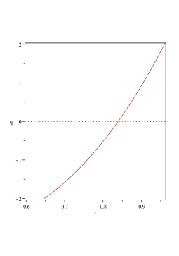
Figure 3: Variation of the deceleration parameter versus the redshift.

Variation of $\dot{H}$ with cosmic time or redshift gives another part of important information about the cosmology of this model. We deduce the relation for variation of $H$ versus the cosmic time as follows

$$\dot{H}=\frac{r\big{(}\dot{f}(R)\alpha(\varphi)+f(R)\dot{\alpha}(\varphi)\big{)}}{8\beta}\Big{[}2\sqrt{1-3b}\,\cosh(\frac{\eta}{3})-1\Big{]}+\frac{rf(R)\alpha(\varphi)}{8\beta}\Big{[}\frac{-3\dot{b}}{\sqrt{1-3b}}\,\cosh(\frac{\eta}{3})+\frac{2}{3}\sqrt{1-3b}\,\dot{\eta}\,\sinh(\frac{\eta}{3})\Big{]}$$ (43)

Figure 4 shows the variation of $\dot{H}$ versus the redshift. Since $\dot{H}<0$ always, the model universe described here will not acquire super-acceleration and big-rip singularity in the future.

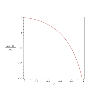
Figure 4: Variation of $\frac{\dot{H}}{H_{0}^{2}}$ versus the redshift.

This example shows how a modified GBIG scenario has the potential to give a phantom-like behavior in a holographic viewpoint. This behavior is realized without introducing any phantom field in this setup. In fact a combination of the curvature effect and the non-minimal coupling provides the suitable framework for realization of this phantom mimicry.

5 Summary

The model presented here, contains the Gauss-Bonnet term as the $UV$ sector of the theory, while the Induced Gravity effect completes the $IR$ side of the model. The induced gravity on the brane is modified in the spirit of $f(R)$ gravity which itself provides the facility to self-accelerate even the normal, ghost-free branch of the DGP-inspired model [11,19]. The model also considers a non-minimal coupling between the canonical scalar field on the brane and the modified induced gravity. This is a general framework for treating dark energy problem and other alternative scenarios can be regarded as subclasses of this general model. We have studied the cosmological dynamics in this generalized braneworld setup within a holographic point of view. By adopting a relatively general ansatz for $f(R)$ gravity (Hu-Sawicki model) on the brane, we have shown that the modified GBIG scenario presented here realizes the phantom-like behavior: the effective energy density increases with cosmic time and the effective equation of state parameter crosses the phantom divide line smoothly in the same way as observations suggest: from quintessence to the phantom phase. We have studied also the holographic nature of the dark energy in this setup by calculation of the effective gravitational constant via a perturbational approach. In this model, $\dot{H}<0$ always, and therefore the model universe described here will not acquire super-acceleration and big-rip singularity in the future.

Acknowledgment
This work has been supported partially by Research Institute for Astronomy and Astrophysics of Maragha, IRAN.

References

-
[1]
S. Perlmutter et al, Astrophys. J. 517 (1999) 565
A. G. Riess et al, Astron. J. 116 (1998) 1006
A. D. Miller et al, Astrophys. J. Lett. 524 (1999) L1
P. de Bernardis et al, Nature 404 (2000) 955
S. Hanany et al, Astrophys. J. Lett. 545 (2000) L5
A. G. Riess et al, Astrophys. J. 607 (2004) 665
P. Astier et al, Astron. Astrophys. 447 (2006) 31
W. M. Wood-Vasey et al, Astrophys. J. 666 (2007) 694
D. N. Spergel et al, Astrophys. J. Suppl 170 (2007) 377
G. Hinshaw et al, Astrophys. J. Suppl , 288 (2007)170
M. Colless et al, Mon. Not. R. Astron. Soc. 328 (2001) 1039
M. Tegmark et al, Phys. Rev. D 69 (2004) 103501
S. Cole et al., Mon. Not. R. Astron. Soc. 362 (2005) 505
V. Springel, C. S. Frenk, and S. M. D. White, Nature (London) 440 (2006) 1137
S. P. Boughn and R. G. Crittenden, Nature 427 (2004) 24
S. P. Boughn and R. G. Crittenden, Mon. Not. R. Astron. Soc. 360 (2005) 1013
P. Fosalba, E. Gaztanaga and F.J. Castander, Astrophys. J. 597 (2003) L89
P. Fosalba, and E. Gaztanaga, Mon. Not. R. Astron. Soc. 350 (2004) L37
J. D. McEwen et al, Mon. Not. R. Astron. Soc. 376 (2007) 1211
M. R. Nolta, Astrophys. J., 608 (2004) 10
P. Vielva et al, Mon. Not. R. Astron. Soc. 365 (2006) 891
C. R. Contaldi, H. Hoekstra, and A. Lewis, Phys. Rev. Lett. 90 (2003) 221303. -
[2]
E. J. Copeland, M. Sami and S. Tsujikawa, Int. J. Mod. Phys. D
15 (2006) 1753, [ arXiv:hep-th/0603057]
M. Sami, Curr. Sci. 97 (2009)887, [arXiv:0904.3445]. -
[3]
S. M. Carroll, Living Rev. Rel. 4 (2001) 1,
[arXiv:astro-ph/0004075]
T. Padmanabhan, Phys. Rept. 380 (2003) 235. -
[4]
S. Nojiri and S. D. Odintsov, Int. J. Geom. Meth. Mod. Phys. 4
(2007) 115, [arXiv:hep-th/0601213]
R. Durrer and R. Maartens, [arXiv:0811.4132]
S. Capozziello and M. Francaviglia, Gen. Rel. Grav. 40 (2008) 357, [arXiv:0706.1146]
T. P. Sotiriou and V. Faraoni, [arXiv:0805.1726]. -
[5]
C. Deffayet, Phys. Lett. B 502 (2001) 199
C. Deffayet, G. Dvali and G. Gabadadze, Phys. Rev. D 65 (2002) 044023
A. Lue, Phys. Rept. 423 (2006) 48. -
[6]
M. Li, Phys. Lett. B 603 (2004) 1
M. Ito, Europhys. Lett. 71 (2005) 712
Y. Gong, B. Wang and Y. -Z. Zhang, Phys. Rev. D72 (2005) 043510
Y. S. Myung, Phys. Lett. B610 (2005) 18
D. Pavon, W. Zimdahl, Phys. Lett. B628 (2005) 206
S. Nojiri and S. D. Odintsov, Gen. Rel. Grav. 38 (2006) 1285
X. Zhang and F. -Q. Wu, Phys. Rev.D 72 (2005) 043524
B. Guberina, R. Horvat and H. Nikolic, Phys. Rev. D 72 (2005) 125011
B. Wang, C. -Y. Lin and E. Abdalla, Phys. Lett. B 637 (2006) 357
B. Hu and Y. Ling, Phys. Rev. D 73 (2006) 123510
M. R. Setare and S. Shafei, JCAP 0609 (2006) 011
W. Zimdahl and D. Pavon, Class. Quant. Grav. 24 (2007) 5461
M. R. Setare, Phys. Lett. B 642 (2006) 421
B. Chen, M. Li and Y. Wang, Nucl. Phys. B 774 (2007) 256
K. Y. Kim, H. W. Lee and Y. S. Myung, Mod. Phys. Lett.A 22 (2007) 2631
B. Wang, C. -Y. Lin, D. Pavon and E. Abdalla, Phys. Lett.B 662 (2008) 1
E. N. Saridakis, Phys. Lett. B 660 (2008) 138-143
M. Li, C. Lin and Y. Wang, JCAP 05 (2008) 023
Y. S. Myung and M. -G. Seo, Phys. Lett.B 671 (2009) 435
R. Horvat, JCAP 0810 (2008) 022
M. R. Setare and E. N. Saridakis, Phys. Lett. B 671 (2009) 331
H. Wei, Nucl. Phys. B 819 (2009) 210, [ arXiv:0902.2030]
E. N. Saridakis, Phys. Lett. B 661 (2008) 335
M. R. Setare and E. N. Saridakis, Phys. Lett.B 670 (2008) 1. -
[7]
S. Nojiri and S. D. Odintsov, [arXiv:0807.0685]
K. Bamba, S. Nojiri and S. D. Odintsov, JCAP 0810 (2008) 045
S. Jhingan, S. Nojiri, S. D. Odintsov, M. Sami, I. Thongkool and S. Zerbini, Phys. Lett.B 663 (2008) 424
G. Cognola, E. Elizalde, S. Nojiri, S. D. Odintsov, L. Sebastiani, S. Zerbini, Phys. Rev. D 77 (2008) 046009
S. Nojiri and S. D. Odintsov, Phys. Lett. B 659 (2008) 821
S. Nojiri and S. D. Odintsov, Phys. Rev. D 77 (2008) 026007. -
[8]
S. Nojiri, S. D. Odintsov and M. Sasaki, Phys. Rev. D 71 (2005)
123509
S. Nojiri and S. D. Odintsov, Phys. Lett. B 631 (2005) 1
S. Nojiri, S. D. Odintsov and O. G. Gorbunova, J. Phys. A39 (2006) 6627
S. Nojiri, S. D. Odintsov and P. V. Tretyakov, Phys. Lett. B 651 (2007) 224
B. Li, J. D. Barrow and D. F. Mota, Phys. Rev. D 76 (2007) 044027. -
[9]
S. Nojiri, S. D. Odintsov and M. Sami, Phys. Rev. D 74 (2006)
046004
D. Konikowska and M. Olechowski, Phys. Rev. D 76 (2007) 124020. - [10] S. Nojiri and S. D. Odintsov, J. Phys. Conf. Ser. 66 (2007) 012005, [arXiv:hep-th/0611071].
-
[11]
K. Nozari and N. Rashidi, JCAP 0909 (2009) 014,
[arXiv:0906.4263]
K. Nozari and N. Rashidi, Int. J. Theor. Phys. 48 (2009) 2800, [ arXiv:0906.3808]
K. Nozari and M. Pourghasemi, JCAP 10 (2008) 044, [arXiv:0808.3701]
K. Nozari and F. Kiani, JCAP 07 (2009) 010, [arXiv:0906.3806]
K. Nozari and T. Azizi, Phys. Lett. B 680 (2009) 205, [arXiv:0909.0351]
K. Nozari, T. Azizi and M. R. Setare, JCAP 10 (2009) 022, [arXiv:0910.0611]
K. Nozari and N. Aliopur, Europhys. Lett. 87 (2009) 69001. - [12] M. Bouhmadi-Lopez and P. V. Moniz, Phys. Rev. D 78 (2008) 084019, [arXiv:0804.4484].
- [13] M. Abramowitz and I. Stegun, Handbook of Mathematical Function, Dover, 1980.
-
[14]
L. Amendola, C. Charmousis and S. C. Davis, JCAP 0612 (2006)
020, [arXiv:hep-th/0506137]
L. Amendola, C. Charmousis, S. C. Davis, JCAP 0710 (2007) 004, [arXiv:0704.0175]. - [15] E. N. Saridakis, JCAP 0804 (2008) 020, [arXiv:0712.2672].
- [16] W. Hu and I. Sawicki, Phys. Rev. D 76 (2007) 064004, [arXiv:0705.1158].
- [17] K. Nozari, JCAP 0709 (2007) 003, [arXiv:0708.1611].
-
[18]
M. Szydlowski, O. Hrycyna and A. Kurek, Phys. Rev. D 77 (2008)
027302, [arXiv:0710.0366]
See also K. Nozari and S. D. Sadatian, Mod. Phys. Lett. A 23(2008) 2933, [arXiv:0710.0058]. - [19] M. Bouhmadi-Lopez, JCAP 0911 (2009) 011, [ arXiv:0905.1962]