Abstract

Bianchi type V string cosmological models with bulk viscosity for massive string are investigated. The bulk viscosity is assumed to vary with time in such a manner that it is related to simple power function of the energy density. Using generation technique (Camci et al., 2001), it is shown that Einstein’s field equations are solvable for any arbitrary cosmic scale function. Solution for particular form of cosmic scale functions are also obtained. It is found that solutions based on generation technique are relevant to the observational results. Some physical and geometrical aspect of the models are also discussed.

PACS: 98.80.cq, 98.80.-k
Key words: Bianchi type V universe, String theory, Bulk viscosity.

1 Introduction

The string theory plays a significant role in the study of physical situation at the very early stages of the formation of the universe. It is generally assumed that after the big bang, the universe may have undergone a series of phase transitions as its temperature lowered down below some critical temperature as predicted by grand unified theories [1]$-$[6]. At the very early stages of evolution of the universe, it is believed that during phase transition the symmetry of the universe is broken spontaneously. It can give rise to topologically stable defects such as domain walls, strings and monopoles [1]. In all these three cosmological structures, only cosmic strings have excited the most interesting consequence [7] because they are believed to give rise to density perturbations which lead to formation of galaxies [4, 8]. These cosmic strings can be closed like loops or open like a hair which move through time and trace out a tube or a sheet, according to whether it is closed or open. The string is free to vibrate and its different vibrational modes present different types of particles carrying the force of gravitation. This is why much interesting to study the gravitational effect that arises from strings by using Einstein’s field equations. The general relativistic treatment of strings has been initially given by Letelier [9, 10] and Stachel [11]. Letelier [9] obtained the general solution of Einstein’s field equations for a cloud of strings with spherical,plane and a particular case of cylindrical symmetry. Letelier [10] also obtained massive string cosmological models in Bianchi type-I and Kantowski-Sachs space-times. Benerjee et al. [12] have investigated an axially symmetric Bianchi type I string dust cosmological model in presence and absence of magnetic field. Exact solutions of string cosmology for Bianchi type II, $VI_{0}$, VIII and IX space-times have been studied by Krori et al. [13] and Wang [14, 15]. Bali and Upadhaya [16] have presented LRS Bianchi type I string dust magnetized cosmological models. Singh and Singh [17] investigated string cosmological models with magnetic field in the context of space-time with $G_{3}$ symmetry. Singh [18, 19], has studied string cosmology with electromagnetic fields in Bianchi type II, VIII and IX space-times.

Bianchi V universes are the natural generalization of FRW models with negative curvature.These open models are favored by the available evidences for low density universes (Gott et al [20]).Bianchi type V cosmological model where matter moves orthogonally to the hypersurface of homogeneity, has been studied by Heckmann and Schucking [21]. Exact tilted solutions for the Bianchi type V space-time are obtained by Hawkings [22], Grishchuk et al. [23]. Ftaclas and Cohen [24] have investigated LRS Bianchi type V universes containing stiff matter with electromagnetic field. Lorentz [25] has investigated LRS Bianchi type V tilted models with stiff fluid and electromagnetic field. Pradhan et al [26] have investigated The generation of Bianchi type V cosmological models with varying $\Lambda$ term. Yadav et al. [27, 28] have investigated bulk viscous string cosmological models in different space-times. Bali and Anjali [29], Bali [30] have obtained Bianchi type-I, and type V string cosmological models in general relativity. The string cosmological models with a magnetic field are discussed by Tikekar and Patel [31], Patel and Maharaj [32]. Ram and Singh [33] obtained some new exact solution of string cosmology with and without a source free magnetic field for Bianchi type I space-time in the different basic form considered by Carminati and McIntosh [34]. Yavuz et al. [35] have examined charged strange quark matter attached to the string cloud in the spherical symmetric space-time admitting one-parameter group of conformal motion. Kaluza-Klein cosmological solutions are obtained by Yilmaz [36] for quark matter attached to the string cloud in the context of general relativity.

The distribution of matter can be satisfactorily described by a perfect fluid due to the large scale distribution of galaxies in our universe. However, observed physical phenomena such as the large entropy per baryon and the remarkable degree of isotropy of the cosmic microwave background radiation, suggest anal- ysis of dissipative effects in cosmology. Furthermore, there are several processes which are expected to give rise to viscous effects. These are the decoupling of neutrinos during the radiation era and the decoupling of radiation and matter during the recombination era. Bulk viscosity is associated with the GUT phase transition and string creation. Misner [37] has studied the effect of viscosity on the evolution of cosmological models. The role of viscosity in cosmology has been investigated by Weinberg [38]. Nightingale [39], Heller and Klimek [40] have obtained a viscous universes without initial singularity. The model stud- ied by Murphy [41] possessed an interesting feature in which big bang type of singularity of infinite space-time curvature does not occur to be a finite past. However, the relationship assumed by Murphy between the viscosity coefficient and the matter density is not acceptable at large density. Thus, we should con- sider the presence of material distribution other than a perfect fluid to obtain a realistic cosmological models (see Gr$\o{}$n [42] for a review on cosmological models with bulk viscosity). The effect of bulk viscosity on the cosmological evolution has been investigated by a number of authors in the framework of general theory of relativity.

2 Field Equations

we consider the Bianchi type V metric of the form

$$ds^{2}=dt^{2}-A^{2}(t)dx^{2}-e^{2\alpha x}[B^{2}(t)dy^{2}+C^{2}(t)dz^{2}]$$ (1)

where $\alpha$ is a constant.
The energy momentum tensor for cloud of string dust with bulk viscous fluid of string given by Landau and Lifshitz (1963) and Letelier (1979)

$$T^{j}_{\;i}=\rho v_{i}v^{j}-\lambda x_{i}x^{j}-\xi v;^{l}_{l}\left(g^{j}_{\;i}+v_{i}v^{j}\right)$$ (2)

where $v_{i}$ and $x_{i}$ satisfy the condition

$$v^{i}v_{i}=-x^{i}x_{i}=1,v^{i}x_{i}=0.$$ (3)

Here $\rho$ is the proper energy density of the cloud of string with particle attached to them.$\lambda$ is the string tension density, $v^{i}$, the four velocity of the particles and $x^{i}$, the unit space vector representing the direction of strings.If the particle density of the configuration is denoted by $\rho_{p}$ then we have

$$\rho=\rho_{p}+\lambda$$ (4)

For the energy momentum tensor (2) and Bianchi type V metric (1), Einstein’s field equations

$$R^{j}_{\;i}-\frac{1}{2}Rg^{j}_{\;i}=-8\pi T^{j}_{\;i}$$ (5)

yield the following five independent equations

$$\frac{\ddot{A}}{A}+\frac{\ddot{B}}{B}+\frac{\dot{A}\dot{B}}{AB}-\frac{\alpha^{2}}{A^{2}}=-8\pi\xi\theta$$ (6)

$$\frac{\ddot{A}}{A}+\frac{\ddot{C}}{C}+\frac{\dot{A}\dot{C}}{AC}-\frac{\alpha^{2}}{A^{2}}=-8\pi\xi\theta$$ (7)

$$\frac{\ddot{B}}{B}+\frac{\ddot{C}}{C}+\frac{\dot{B}\dot{C}}{BC}-\frac{\alpha^{2}}{A^{2}}=-8\pi\left(\lambda+\xi\theta\right)$$ (8)

$$\frac{\dot{A}\dot{B}}{AB}+\frac{\dot{A}\dot{C}}{AC}+\frac{\dot{B}\dot{C}}{BC}-\frac{3\alpha^{2}}{A^{2}}=-8\pi\rho$$ (9)

$$\frac{2\dot{A}}{A}-\frac{\dot{B}}{B}-\frac{\dot{C}}{C}=0$$ (10)

Here and what follows the dots overhead the symbol A, B, C denotes differentiation with respect to t.
The physical quantities expansion scalar $\theta$ and shear scalar $\sigma^{2}$ have the following expressions

$$\theta=\frac{\dot{A}}{A}+\frac{\dot{B}}{B}+\frac{\dot{C}}{C}$$ (11)

$$\sigma^{2}=\frac{1}{2}\sigma_{ij}\sigma^{ij}=\frac{1}{3}\left[\theta^{2}-\frac{\dot{A}\dot{B}}{AB}-\frac{\dot{A}\dot{C}}{AC}-\frac{\dot{B}\dot{C}}{BC}\right]$$ (12)

Integrating eqs.(10) and absorbing the integrating constant into B or C, we obtain

$$A^{2}=BC$$ (13)

without loss of any generality. Now subtracting equation $(7)$ from $(6)$, we obtain

$$2\frac{\ddot{B}}{B}+\left(\frac{\dot{B}}{B}\right)^{2}=2\frac{\ddot{C}}{C}+\left(\frac{\dot{C}}{C}\right)^{2}$$ (14)

which on integration yields

$$\frac{\dot{B}}{B}-\frac{\dot{C}}{C}=\frac{k}{(BC)^{\frac{3}{2}}}$$ (15)

where k is the constant of integration. Hence for the metric function B or C from the above first order differential eqs.(15), some scale transformations permit us to obtain new metric function B or C.
    Firstly, under the scale transformation $dt=B^{\frac{1}{2}}dT$, equation $(15)$ takes the form

$$CB_{T}-BC_{T}=kC^{-\frac{1}{2}}$$ (16)

where the subscript represents derivative with respect to $T$. Considering eqs.(16) as a linear differential equation for B, where C is an arbitrary function, we obtain

$$(i)\;\;\;\;\;\;\;\;B=k_{1}C+kC\int{\frac{dT}{C^{\frac{5}{2}}}},$$ (17)

where $k_{1}$ is the the constant of integration. Similarly, using the transformation $dt=B^{\frac{3}{2}}d\bar{T}$, $dt=C^{\frac{1}{2}}d\tilde{t}$ and $dt=C^{\frac{3}{2}}d\tau$ in equation (13) after some algebra we obtain respectively.

$$(ii)\;\;\;\;\;\;\;\;\;\;B(\bar{T})=k_{2}Ce^{\left(k\int\frac{d\bar{T}}{C^{\frac{3}{2}}}\right)},$$ (18)

$$(iii)\;\;\;\;\;\;\;\;\;\;\;C(\tilde{t})=k_{3}B-kB\int\frac{d\tilde{t}}{B^{\frac{5}{2}}},$$ (19)

$$(iv)\;\;\;\;\;\;\;\;\;\;\;\;C(\tau)=k_{4}Be^{\left(k\int\frac{d\tau}{B^{\frac{3}{2}}}\right)},$$ (20)

where $k_{2}$,$k_{3}$ and $k_{4}$ are constant of integration. Thus choosing any given function B or C in cases (i), (ii), (iii) and (iv), one can obtain B or C.

3 Generation technique for solution

We consider the following four cases

3.1 Case (i): $C=T^{n}$  (n is a real number satisfying $n\neq\frac{2}{5}$)

In this case equation (15) gives

$$B=k_{1}T^{n}+\frac{2k}{2-5n}T^{{1}-\frac{3n}{2}}$$ (21)

and then equation (11), we obtain

$$A^{2}=k_{1}T^{2n}+\frac{2k}{2-5n}T^{1-\frac{n}{2}}$$ (22)

Hence metric (1) reduces to the following form

$$ds^{2}=(k_{1}T^{n}+2lT^{l_{1}})[dT^{2}-T^{n}dx^{2}]-e^{2\alpha x}\left[\left(k_{1}T^{n}+2lT^{l_{1}}\right)^{2}dy^{2}+T^{2n}dz^{2}\right],$$ (23)

where $l=\frac{k}{2-5n}$ and $l_{1}=1-\frac{3n}{2}$
In this case the physical parameters, i.e. the string tension density $(\lambda)$, the energy density $(\rho)$, the particle density $(\rho_{p})$ and the kinematical parameters, i.e. the scalar of expansion $(\theta)$, shear scalar $(\sigma)$ and the proper volume $(V^{3})$ for model $(23)$ are given by

$$8\pi\lambda=\left[-2k_{1}^{2}n(n-1)T^{2n-2}-k_{1}ln(10-13n){T^{-(l_{1}+2n)}}-\frac{1}{2}l^{2}(4+4n-11n^{2}){T}^{-3n}\right]\psi_{1}^{-3}$$

$$+\alpha^{2}{T}^{-n}\psi_{1}^{-1}+24\pi\xi\left[k_{1}nT^{n-1}+\frac{1}{2}l(2-n)T^{\frac{-3n}{2}}\right]\psi_{1}^{-\frac{3}{2}},$$ (24)

$$8\pi\rho=\left[3k_{1}^{2}n^{2}T^{2n-2}+3k_{1}ln(2-n)T^{-(l_{1}+2n)}+\frac{1}{2}l^{2}(4+4n-11n^{2})T^{-3n}\right]\psi_{1}^{-3}$$

$$-3\alpha^{2}T^{-n}\psi_{1}^{-1},$$ (25)

$$8\pi\rho_{p}=\left[n(5n-2)k_{1}^{2}T^{2n-2}+16k_{1}ln(1-n)T^{-(l_{1}+2n)}+l^{2}(4+4n-11n^{2})T^{-3n}\right]\psi_{1}^{-3}$$

$$-4\alpha^{2}T^{n}\psi_{1}^{-1}-24\pi\xi\left[k_{1}nT^{n-1}+\frac{1}{2}l(2-n)T^{\frac{-3n}{2}}\right]\psi_{1}^{-\frac{3}{2}}$$ (26)

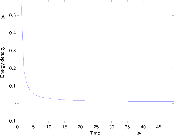
Figure 1: The plot of energy density $\rho$ vs. time T with parameters $n=0.5,k=1,\alpha=1k_{1}=1,l_{1}=0.25$

Where $\psi_{1}=\left(k_{1}T^{n}+2lT^{l_{1}}\right)$.
This general solution has a rich structure and admits many numbers of solutions by suitable choice of $\xi(t)$. Here the choice of $\xi(t)$ is quite arbitrary but since we look for physically viable model of universe thus for specification of $\xi$, in most of the investigations, involving bulk viscosity, it is assumed to be simple power function of energy density (Pavon [43] , Maartens [44] and Zimdahl [45]).

$$\xi(t)=\xi_{0}\rho^{w}$$ (27)

Where $\xi_{0}$ and $w$ are constant. Now we consider two cases depending on two values of w, namely $0$ and $1$.

3.1.1 Case I:  Solution for $\xi=\xi_{0}$

For $w=0$, eqs.(27) reduces $\xi=\xi_{0}$.Thus eqs.(24) and eqs.(26) reduces to

$$8\pi\lambda=\left[-2k_{1}^{2}n(n-1)T^{2n-2}-k_{1}ln(10-13n){T^{-(l_{1}+2n)}}-\frac{1}{2}l^{2}(4+4n-11n^{2}){T}^{-3n}\right]\psi_{1}^{-3}$$

$$+\alpha^{2}{T}^{-n}\psi_{1}^{-1}+24\pi\xi_{0}\left[k_{1}nT^{n-1}+\frac{1}{2}l(2-n)T^{\frac{-3n}{2}}\right]\psi_{1}^{-\frac{3}{2}},$$ (28)

$$8\pi\rho_{p}=\left[n(5n-2)k_{1}^{2}T^{2n-2}+16k_{1}ln(1-n)T^{-(l_{1}+2n)}+l^{2}(4+4n-11n^{2})T^{-3n}\right]\psi_{1}^{-3}$$

$$-4\alpha^{2}T^{n}\psi_{1}^{-1}-24\pi\xi_{0}\left[k_{1}nT^{n-1}+\frac{1}{2}l(2-n)T^{\frac{-3n}{2}}\right]\psi_{1}^{-\frac{3}{2}}$$ (29)

3.1.2 Case II:  Solution for $\xi=\xi_{0}\rho$

For $w=1$, eqs.(27) reduces $\xi=\xi_{0}\rho$, with use of eqs.(25), eqs.(24) and eqs.(26) reduces to

$$8\pi\lambda=\left[-2k_{1}^{2}n(n-1)T^{2n-2}-k_{1}ln(10-13n){T^{-(l_{1}+2n)}}-\frac{1}{2}l^{2}(4+4n-11n^{2}){T}^{-3n}\right]\psi_{1}^{-3}$$

$$+\alpha^{2}{T}^{-n}\psi_{1}^{-1}-9\xi_{0}\alpha^{2}T^{-n}\left(k_{1}nT^{n-1}+\frac{1}{2}l(2-n)T^{\frac{-3n}{2}}\right)\psi_{1}^{-\frac{5}{2}}+$$

$$3\xi_{0}\left(3k_{1}^{2}n^{2}T^{2n-2}+3k_{1}ln(2-n)T^{-(l_{1}+2n)}+\frac{1}{2}l^{2}(4+4n-11n^{2})T^{-3n}\right)\psi_{1}^{-3}$$

$$\left(k_{1}nT^{n-1}+\frac{1}{2}l(2-n)T^{\frac{-3n}{2}}\right)\psi_{1}^{-\frac{3}{2}}$$ (30)

$$8\pi\rho_{p}=\left[n(5n-2)k_{1}^{2}T^{2n-2}+16k_{1}ln(1-n)T^{-(l_{1}+2n)}+l^{2}(4+4n-11n^{2})T^{-3n}\right]\psi_{1}^{-3}$$

$$-4\alpha^{2}T^{n}\psi_{1}^{-1}+9\xi_{0}\alpha^{2}T^{-n}\left(k_{1}nT^{n-1}+\frac{1}{2}l(2-n)T^{\frac{-3n}{2}}\right)\psi_{1}^{-\frac{5}{2}}-$$

$$3\xi_{0}\left(3k_{1}^{2}n^{2}T^{2n-2}+3k_{1}ln(2-n)T^{-(l_{1}+2n)}+\frac{1}{2}l^{2}(4+4n-11n^{2})T^{-3n}\right)\psi_{1}^{-3}$$

$$\left(k_{1}nT^{n-1}+\frac{1}{2}l(2-n)T^{\frac{-3n}{2}}\right)\psi_{1}^{-\frac{3}{2}}$$ (31)

From Eqs.(25), we note that $\rho(t)$ is a decreasing function of time and $\rho>0$ for all times. This behaviour is clearly depicted in Fig. 1 as a representative case with appropriate choice of constants of integration and other physical parameters using reasonably well known situations. Figures 1 show this physical behaviours of energy density as a decreasing functions of time. Also it is observed that bulk viscosity affect the string tension density $\lambda$ and particle density $\rho_{p}$.

$$\theta=3\left[k_{1}nT^{n-1}+\frac{1}{2}l(2-n)T^{\frac{-3n}{2}}\right]\psi_{1}^{-\frac{3}{2}}$$ (32)

$$\sigma=\frac{1}{2}kT^{-\frac{3n}{2}}\psi_{1}^{-\frac{3}{2}}~{}~{}~{}~{}~{}~{}~{}~{}~{}~{}~{}~{}~{}~{}~{}~{}~{}~{}~{}~{}~{}~{}~{}~{}~{}~{}~{}~{}~{}~{}$$ (33)

$$V^{3}=\left(k_{1}T^{2n}+2lT^{n+l_{1}}\right)^{\frac{3}{2}}e^{2\alpha x}~{}~{}~{}~{}~{}~{}~{}~{}~{}~{}~{}~{}~{}~{}~{}~{}~{}~{}~{}~{}~{}~{}~{}~{}~{}~{}~{}~{}~{}~{}$$ (34)

Equations (32) and (33) leads to

$$\frac{\sigma}{\theta}=\frac{1}{6}k\left[k_{1}nT^{n-l_{1}}+\frac{1}{2}l(2-n)\right]^{-1}~{}~{}~{}~{}~{}~{}~{}~{}~{}~{}~{}~{}~{}~{}~{}~{}~{}~{}~{}~{}~{}~{}~{}$$ (35)

The energy condition $\rho\geq 0$ and $\rho_{p}\geq 0$ satisfy for model (23). The condition $\rho\geq 0$ and $\rho_{p}\geq 0$ leads to

$$\left[3k_{1}^{2}n^{2}T^{3n-2}+3k_{1}ln(2-n)T^{-(l_{1}+n)}+\frac{1}{2}l^{2}\left(4+4n-11n^{2}\right)T^{-2n}\right]$$

$$\psi_{1}^{-2}\geq{3\alpha}^{2}$$ (36)

$$\left[n(2-5n)k_{1}^{2}T^{n-2}+16k_{1}ln(n-1)T^{-(l_{1}+3n)}+l^{2}\left(11n^{2}-4n-4\right)T^{-4n}\right]$$

$$\psi_{1}^{-2}-24\pi\xi\left(k_{1}nT^{-1}+\frac{1}{2}l(2-n)T^{-\frac{5n}{2}}\right)\psi^{-\frac{1}{2}}\geq{4\alpha}^{2}$$ (37)

respectively.
We observe that the string tension density $\lambda\geq 0$, leads to

$$\left[-2k_{1}^{2}n(n-1)T^{3n-2}-k_{1}ln(10-13n)T^{-(l_{1}+n)}-\frac{1}{2}l^{2}\left(4+4n-11n^{2}\right)T^{-2n}\right]\psi_{1}^{-2}$$

$$+24\pi\xi\left[k_{1}nT^{2n-1}+\frac{1}{2}l(2-n)T^{\frac{-n}{2}}\right]\psi_{1}^{-\frac{1}{2}}\geq{-\alpha}^{2}$$ (38)

Generally the model$(23)$ are expanding, shearing and approaches to isotropy at late time. For $k=0$, the model becomes shear free. We observe that as $T\rightarrow\infty$, $V^{3}\rightarrow\infty$ and $\rho\rightarrow 0$ hence volume increases when T increases and the proper energy density of the cloud of string with particle attached to them is the decreasing function of time.

3.2 case(ii): $C={\bar{T}}^{n}$  (n is a real number satisfying $n\neq\frac{2}{3}$)

In this case equation (18) gives

$$B=k_{2}{\bar{T}}^{n}e^{M{\bar{T}}^{l_{1}}}$$ (39)

and from equation (13), we obtain

$$A^{2}=k_{2}{\bar{T}}^{2n}e^{M{\bar{T}}^{l_{1}}}$$ (40)

where $M=\frac{k}{l_{1}}$. Hence the metric (1) reduces to the form

$$ds^{2}={\bar{T}}^{\frac{4(1-l_{1})}{3}}\left[{\bar{T}}^{\frac{2(1-l_{1})}{3}}e^{3M{\bar{T}}^{l_{1}}}d{\bar{T}^{2}}-e^{M{\bar{T}}^{l_{1}}}dx^{2}-e^{2\alpha x}\left(e^{2M{\bar{T}}^{l_{1}}}dy^{2}+dz^{2}\right)\right],$$ (41)

where the constant $k_{2}$ is taken, without loss of generality, equal to $1$. In this case the physical parameters, i.e. the string tension density $(\lambda)$, the energy density $(\rho)$, the particle density $(\rho_{p})$ and the kinematical parameters, i.e. the scalar of expansion $(\theta)$, shear scalar $(\sigma)$ and the proper volume $(V^{3})$ for model (41) are given by

$$8\pi\lambda=2n{\bar{T}}^{2(l_{1}-2)}+3nk{\bar{T}}^{3l_{1}-4}+\frac{1}{2}k^{2}{\bar{T}}^{4(l_{1}-1)}+\alpha^{2}{\bar{T}}^{\frac{4(l_{1}-1)}{3}}e^{-3M\bar{T}^{l_{1}}}$$

$$+24\pi\xi\left(n{\bar{T}}^{l_{1}-2}+\frac{1}{2}k{\bar{T}}^{2(l_{1}-1)}\right)$$ (42)

$$8\pi\rho=3n^{2}{\bar{T}}^{2(l_{1}-2)}+3nk{\bar{T}}^{3l_{1}-4}+\frac{1}{2}k^{2}{\bar{T}}^{4(l_{1}-1)}-3\alpha^{2}{\bar{T}}^{\frac{4(l_{1}-1)}{3}}e^{-3M\bar{T}^{l_{1}}},$$ (43)

$$8\pi\rho_{p}=n(3n-2){\bar{T}}^{2(l_{1}-2)}-4\alpha^{2}{\bar{T}}^{\frac{4(l_{1}-1)}{3}}e^{3M\bar{\bar{T}}^{l_{1}}}-24\pi\xi\left(n{\bar{T}}^{l_{1}-2}+\frac{1}{2}k{\bar{T}}^{2(l_{1}-1)}\right)$$ (44)

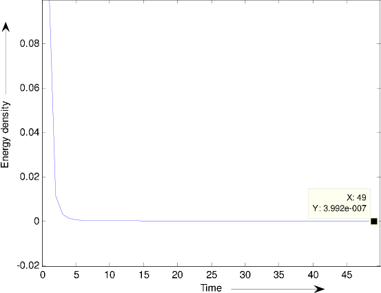
Figure 2: The plot of energy density $\rho$ vs. time $\bar{T}$ with parameters $n=0.5,k=1,\alpha=1k_{1}=1,l_{1}=0.25$

3.2.1 Case I:  Solution for $\xi=\xi_{0}$

For $w=0$, eqs.(27) reduces $\xi=\xi_{0}$.Thus eqs.(42) and eqs.(44) reduces to

$$8\pi\lambda=2n{\bar{T}}^{2(l_{1}-2)}+3nk{\bar{T}}^{3l_{1}-4}+\frac{1}{2}k^{2}{\bar{T}}^{4(l_{1}-1)}+\alpha^{2}{\bar{T}}^{\frac{4(l_{1}-1)}{3}}e^{-3M\bar{T}^{l_{1}}}+$$

$$24\pi\xi_{0}\left[n{\bar{T}}^{l_{1}-2}+\frac{1}{2}k{\bar{T}}^{2(l_{1}-1)}\right]$$ (45)

$$8\pi\rho_{p}=n(3n-2){\bar{T}}^{2(l_{1}-2)}-4\alpha^{2}{\bar{T}}^{\frac{4(l_{1}-1)}{3}}e^{3M\bar{\bar{T}}^{l_{1}}}-24\pi\xi_{0}\left[n{\bar{T}}^{l_{1}-2}+\frac{1}{2}k{\bar{T}}^{2(l_{1}-1)}\right]$$ (46)

3.2.2 Case II:  Solution for $\xi=\xi_{0}\rho$

For $w=1$, eqs.(27) reduces $\xi=\xi_{0}\rho$, with use of eqs.(43), eqs.(42) and eqs.(44) reduces to

$$8\pi\lambda=2n{\bar{T}}^{2(l_{1}-2)}+3nk{\bar{T}}^{3l_{1}-4}+\frac{1}{2}k^{2}{\bar{T}}^{4(l_{1}-1)}+\alpha^{2}{\bar{T}}^{\frac{4(l_{1}-1)}{3}}e^{-3M\bar{T}^{l_{1}}}+$$

$$3\xi_{0}\left[3n^{2}{\bar{T}}^{2(l_{1}-2)}+3nk{\bar{T}}^{3l_{1}-4}+\frac{1}{2}k^{2}{\bar{T}}^{4(l_{1}-1)}-3\alpha^{2}{\bar{T}}^{\frac{4(l_{1}-1)}{3}}e^{-3M\bar{T}^{l_{1}}}\right]$$

$$\left(n{\bar{T}}^{l_{1}-2}+\frac{1}{2}k{\bar{T}}^{2(l_{1}-1)}\right)$$ (47)

$$8\pi\rho_{p}=n(3n-2){\bar{T}}^{2(l_{1}-2)}-4\alpha^{2}{\bar{T}}^{\frac{4(l_{1}-1)}{3}}e^{3M{\bar{T}}^{l_{1}}}-3\xi_{0}\left(n{\bar{T}}^{l_{1}-2}+\frac{1}{2}k{\bar{T}}^{2(l_{1}-1)}\right)$$

$$\left[3n^{2}{\bar{T}}^{2(l_{1}-2)}+3nk{\bar{T}}^{3l_{1}-4}+\frac{1}{2}k^{2}{\bar{T}}^{4(l_{1}-1)}-3\alpha^{2}{\bar{T}}^{\frac{4(l_{1}-1)}{3}}e^{-3M\bar{T}^{l_{1}}}\right]$$ (48)

From Eqs.(43), we note that $\rho(t)$ is a decreasing function of time and $\rho>0$ for all times. This behaviour is clearly shown in Fig. 2. Also it is observed that bulk viscosity affect the string tension density $\lambda$ and particle density $\rho_{p}$.

$$\theta=3\left[n{\bar{T}}^{l_{1}-2}+\frac{1}{2}k{\bar{T}}^{2(l_{1}-1)}\right],$$ (49)

$$\sigma=\frac{1}{2}k\bar{T}^{2(l_{1}-1)}e^{-3M\bar{T}^{l_{1}}}$$ (50)

$$V^{3}=\left(k_{3}\bar{T}^{2n}e^{{M}\bar{T}^{l_{1}}}\right)^{\frac{3}{2}}e^{2\alpha x}$$ (51)

From equation (49) and (50) leads to

$$\frac{\sigma}{\theta}=\frac{k}{6(n\bar{T}^{-l_{1}}+\frac{1}{2}k)}$$ (52)

The energy condition $\rho\geq 0$ and $\rho_{p}\geq 0$ are satisfy for model (36). The condition $\rho\geq 0$ and $\rho_{p}\geq 0$ leads to

$$e^{3M\bar{T}^{l_{1}}}\left[3n^{2}\bar{T}^{\frac{2l_{1}-8}{3}}+3nk\bar{T}^{\frac{5l_{1}-8}{3}}+\frac{1}{2}k^{2}\bar{T}^{\frac{8l_{1}-8}{3}}\right]\geq 3\alpha^{2}$$ (53)

$${\bar{T}}^{\frac{(1-4l_{1})}{3}}e^{-3M\bar{\bar{T}}^{l_{1}}}\left[n(3n-2){\bar{T}}^{2(l_{1}-2)}-24\pi\xi\left(n{\bar{T}}^{l_{1}-2}+\frac{1}{2}k{\bar{T}}^{2(l_{1}-1)}\right)\right]\geq 4\alpha^{2}$$ (54)

respectively.
we observe that the string tension density $\lambda\geq 0$, leads to

$${\bar{T}}^{\frac{(1-4l_{1})}{3}}e^{3M\bar{T}^{l_{1}}}\times$$

$$\left[2n{\bar{T}}^{2(l_{1}-2)}+3nk{\bar{T}}^{3l_{1}-4}+\frac{1}{2}k^{2}{\bar{T}}^{4(l_{1}-1)}+24\pi\xi\left(n{\bar{T}}^{l_{1}-2}+\frac{1}{2}k{\bar{T}}^{2(l_{1}-1)}\right)\right]\geq-\alpha^{2}$$ (55)

For $l_{1}>2$, model (41) is expanding and for $l_{1}<2$, model starts with big bang singularity. Generally the model is expanding, shearing and approaches isotropy at late time. For $k=0$, the model becomes shear free. We observe that as $\bar{T}\rightarrow\infty$, $V^{3}\rightarrow\infty$ and $\rho\rightarrow 0$ hence volume increases when $\bar{T}$ increases and the proper energy density of the cloud of string with particle attached to them is the decreasing function of time.

3.3 Case(iii): $B={\tilde{t}}^{n}$  (n is a real number)

In this case equation (19) gives and

$$C=k_{3}{\tilde{t}^{n}}-2l{\tilde{t}}^{l_{1}}$$ (56)

$$A^{2}=k_{3}{\tilde{t}}^{2n}-2l{\tilde{t}}^{l_{1}+n}$$ (57)

Hence the metric $(1)$ takes the new form

$$ds^{2}=\left(k_{3}{\tilde{t}}^{n}-2l{\tilde{t}}^{l_{1}}\right)\left[dt^{2}-{\tilde{t}}^{n}dx^{2}\right]-e^{2\alpha x}\left[{\tilde{t}}^{2n}dy^{2}+\left(k_{3}{\tilde{t}}^{n}-2l{\tilde{t}}^{l_{1}}\right)^{2}dz^{2}\right],$$ (58)

In this case the physical parameters, i.e. the string tension density $(\lambda)$, the energy density $(\rho)$, the particle density $(\rho_{p})$ and the kinematical parameters, i.e. the scalar of expansion $(\theta)$, shear scalar $(\sigma)$ and the proper volume $(V^{3})$ for model (58) are given by

$$8\pi\lambda=\left[-\frac{1}{2}l^{2}(11n^{2}-4n-4){\tilde{t}}^{-3n}+lk_{3}n(13n-10){\tilde{t}}^{l_{1}+n}-2k_{3}^{2}n(n-1){\tilde{t}}^{2n-2}\right]\psi_{2}^{-3}$$

$$+\alpha^{2}{\tilde{t}}^{-n}\psi_{2}^{-1}+24\pi\xi\left(\frac{1}{2}l(n-2){\tilde{t}}^{-\frac{3n}{2}}+k_{3}n\tilde{t}^{n-1}\right)\psi_{2}^{-\frac{3}{2}},$$ (59)

$$8\pi\rho=\left[-\frac{1}{2}l^{2}(11n^{2}-4n-4){\tilde{t}}^{-3n}-3lk_{3}n(2-n){\tilde{t}}^{l_{1}+n}+3k_{3}^{2}n^{2}{\tilde{t}}^{2n-2}\right]\psi_{2}^{-3}-$$

$$3\alpha^{2}{\tilde{t}}^{-n}\psi_{2}^{-1}$$ (60)

$$8\pi\rho_{p}=\psi_{2}^{-3}\left[n(5n-2)k_{3}^{2}\tilde{t}^{2n-2}-lk_{3}n(12n-8)\tilde{t}^{l_{1}+n}\right]-4\alpha^{2}\tilde{t}^{n}\psi_{2}^{-1}-$$

$$24\pi\xi\left(\frac{1}{2}l(n-2){\tilde{t}}^{-\frac{3n}{2}}+k_{3}n\tilde{t}^{n-1}\right)\psi_{2}^{-\frac{3}{2}},$$ (61)

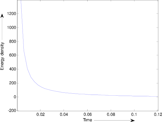
Figure 3: The plot of energy density $\rho$ vs. time $\bar{T}$ with parameters $n=0.5,k=1,\alpha=1k_{1}=1,l_{1}=0.25$

3.3.1 Case I:  Solution for $\xi=\xi_{0}$

For $w=0$, eqs.(27) reduces $\xi=\xi_{0}$.Thus eqs.(59) and eqs.(61) reduces to

$$8\pi\lambda=\left[-\frac{1}{2}l^{2}(11n^{2}-4n-4){\tilde{t}}^{-3n}+lk_{3}n(13n-10){\tilde{t}}^{l_{1}+n}-2k_{3}^{2}n(n-1){\tilde{t}}^{2n-2}\right]\psi_{2}^{-3}$$

$$+\alpha^{2}{\tilde{t}}^{-n}\psi_{2}^{-1}+24\pi\xi_{0}\left(\frac{1}{2}l(n-2){\tilde{t}}^{-\frac{3n}{2}}+k_{3}n\tilde{t}^{n-1}\right)\psi_{2}^{-\frac{3}{2}},$$ (62)

$$8\pi\rho_{p}=\psi_{2}^{-3}\left[n(5n-2)k_{3}^{2}\tilde{t}^{2n-2}-lk_{3}n(12n-8)\tilde{t}^{l_{1}+n}\right]-4\alpha^{2}\tilde{t}^{n}\psi_{2}^{-1}-$$

$$24\pi\xi_{0}\left[\frac{1}{2}l(n-2){\tilde{t}}^{-\frac{3n}{2}}+k_{3}n\tilde{t}^{n-1}\right]\psi_{2}^{-\frac{3}{2}},$$ (63)

3.3.2 Case II:  Solution for $\xi=\xi_{0}\rho$

For $w=1$, eqs.(27) reduces $\xi=\xi_{0}\rho$, with use of eqs.(59), eqs.(61) and eqs.(44) reduces to

$$8\pi\lambda=\left[-\frac{1}{2}l^{2}(11n^{2}-4n-4){\tilde{t}}^{-3n}+lk_{3}n(13n-10){\tilde{t}}^{l_{1}+n}-2k_{3}^{2}n(n-1){\tilde{t}}^{2n-2}\right]\psi_{2}^{-3}$$

$$+\alpha^{2}{\tilde{t}}^{-n}\psi_{2}^{-1}-9\xi_{0}\left(\frac{1}{2}l(n-2){\tilde{t}}^{-\frac{3n}{2}}+k_{3}n\tilde{t}^{n-1}\right)\psi_{2}^{-\frac{5}{2}}+$$

$$3\xi_{0}\left[-\frac{1}{2}l^{2}(11n^{2}-4n-4){\tilde{t}}^{-3n}-3lk_{3}n(2-n){\tilde{t}}^{l_{1}+n}+3k_{3}^{2}n^{2}{\tilde{t}}^{2n-2}\right]\psi_{2}^{-3}\times$$

$$\left(\frac{1}{2}l(n-2){\tilde{t}}^{-\frac{3n}{2}}+k_{3}n\tilde{t}^{n-1}\right)\psi_{2}^{-\frac{3}{2}},$$ (64)

$$8\pi\rho_{p}=\psi_{2}^{-3}\left[n(5n-2)k_{3}^{2}\tilde{t}^{2n-2}-lk_{3}n(12n-8)\tilde{t}^{l_{1}+n}\right]-4\alpha^{2}\tilde{t}^{n}\psi_{2}^{-1}+$$

$$9\xi_{0}\left(\frac{1}{2}l(n-2){\tilde{t}}^{-\frac{3n}{2}}+k_{3}n\tilde{t}^{n-1}\right)\psi_{2}^{-\frac{5}{2}}-3\xi_{0}\left(\frac{1}{2}l(n-2){\tilde{t}}^{-\frac{3n}{2}}+k_{3}n\tilde{t}^{n-1}\right)\psi_{2}^{-\frac{3}{2}}\times$$

$$\left[-\frac{1}{2}l^{2}(11n^{2}-4n-4){\tilde{t}}^{-3n}-3lk_{3}n(2-n){\tilde{t}}^{l_{1}+n}+3k_{3}^{2}n^{2}{\tilde{t}}^{2n-2}\right]\psi_{2}^{-3},$$ (65)

From Eqs.(60), we note that $\rho(t)$ is a decreasing function of time This behaviour is clearly shown in Fig. 3. Also it is observed that bulk viscosity affect the string tension density $\lambda$ and particle density $\rho_{p}$.

$$\theta=3\left[\frac{1}{2}l(n-2){\tilde{t}}^{-\frac{3n}{2}}+k_{3}n\tilde{t}^{n-1}\right]\psi_{2}^{-\frac{3}{2}},$$ (66)

$$\sigma=\frac{1}{2}k{\tilde{t}}^{\frac{-3n}{2}}\psi_{2}^{-\frac{3}{2}},$$ (67)

$$V^{3}=\left(k_{3}{\tilde{t}}^{2n}-2l{\tilde{t}}^{l_{1}+n}\right)^{\frac{3}{2}}e^{2\alpha x}~{}~{}~{}~{}~{}~{}~{}~{}~{}~{}~{}~{}~{}~{}~{}~{}~{}~{}~{}~{}~{}~{}~{}~{}~{}~{}~{}~{}$$ (68)

Equation (66) and (54) leads to

$$\frac{\sigma}{\theta}=\frac{k}{6}\left[k_{3}n{\tilde{t}}^{-(l_{1}+n)}+\frac{l(n-2)}{2}\right]^{-1}$$ (69)

Where $\psi_{2}=\left(k_{3}{\tilde{t}}^{n}-2l{\tilde{t}}^{l_{1}}\right)$.
The energy condition $\rho\geq 0$ and $\rho_{p}\geq 0$ are satisfy for model (58). The condition $\rho\geq 0$ and $\rho_{p}\geq 0$ leads to

$$\left[-\frac{1}{2}l^{2}\left(11n^{2}-4n-4\right)\tilde{t}^{-2n}-3lk_{3}n(2-n)\tilde{t}^{l_{1}+2n}+3k_{3}^{2}n^{2}\tilde{t}^{(3n-2)}\right]\psi_{2}^{-2}\geq 3\alpha^{2}$$ (70)

$$\left(k_{3}\tilde{t}^{n}-2l\tilde{t}^{l_{1}}\right)^{-2}\left[n(5n-2)k_{3}^{2}\tilde{t}^{n-2}-lk_{3}n(12n-8)\tilde{t}^{l}_{1}\right]-24\pi\xi\times$$

$$\left[\frac{1}{2}l(n-2){\tilde{t}}^{-\frac{n}{2}}+k_{3}n\tilde{t}^{-1}\right]\psi_{2}^{-\frac{1}{2}}\geq 4\alpha^{2}$$ (71)

respectively.
We observe that the string tension density $\lambda\geq 0$, leads to

$$\left[-\frac{1}{2}l^{2}\left(11n^{2}-4n-4\right)\tilde{t}^{-2n}+lk_{3}(13n-10)\tilde{t}^{l_{1}+2n}-2k_{3}^{2}n(n-1)\tilde{t}^{3n-2}\right]\times$$

$$\psi_{2}^{-2}+24\pi\xi\left[\frac{1}{2}l(n-2){\tilde{t}}^{-\frac{n}{2}}+k_{3}n\tilde{t}^{-1}\right]\psi_{2}^{-\frac{1}{2}}\geq-\alpha^{2}$$ (72)

Thus we see that the model (58) is generally expanding, shearing and approaches to isotropy at late time. For $k=0$,the model becomes shear free. We observe that as $\tilde{t}\rightarrow\infty$, $V^{3}\rightarrow\infty$ and $\rho\rightarrow 0$ hence volume increases when $\tilde{t}$ increases and the proper energy density of the cloud of string with particle attached to them is the decreasing function of time.

3.4 Case(iv): $B=\tau^{n}$   (n is any real number)

In this case equation (20) gives

$$C=k_{4}\tau^{n}e^{\left(\frac{k}{l_{1}}\tau^{l_{1}}\right)}$$ (73)

and then from equation (13) we obtain

$$A^{2}=k_{4}\tau^{2n}e^{\left(\frac{k}{l_{1}}\tau^{l_{1}}\right)}$$ (74)

Hence the metric (1) reduces to

$$ds^{2}=\tau^{2n}e^{\left(\frac{k}{l_{1}}\tau^{l_{1}}\right)}\left[\tau^{n}e^{\left(\frac{2k}{l_{1}}\tau^{l_{1}}\right)}d\tau^{2}-dx^{2}\right]-e^{2\alpha x}\left[dy^{2}+e^{\left(\frac{2k}{l_{1}}\tau^{l_{1}}\right)}dz^{2}\right],$$ (75)

where without any loss of generality the constant $k_{4}$ is taken equal to $1$. Here we see that the metric function A, B, and C are exponential type function as that of in case $(ii)$. Thus we conclude that physical and geometrical properties of the model are similar to model (41).

4 Conclusion

If we choose $\alpha=0$, metric $(1)$ becomes Bianchi type I metric, studied by several authors in different context. In this paper, we have applied the generation technique followed by Camci et al [46] and found string cosmological models with bulk viscosity. It is shown that the Einstein’s field equation are solvable for an arbitrary cosmic scale function. Starting from a particular cosmic function, new classes of spatially homogeneous and anisotropic cosmological models have been investigated for which the string fluid are acceleration and rotation free but they do have expansion and shear. It is also observed that the physical and geometrical behavior of models in all cases are similar. Generally the model are expanding, shearing and non rotating. All the models are isotropized at late time. Also we found that in all cases energy density is decreasing function of time thus bulk viscosity decreases with time as it is assumed to be simple power function of energy density.

In case $(i)$, for $n\geq 1$, model (23) start expanding with big bang singularity and for $n\leq 0$, model (23) preserve expanding nature as $T\rightarrow 0$, $\theta\rightarrow 0$ and $T\rightarrow\infty$, $\theta\rightarrow\infty$. It is also observed that for $k=0$, shear scalar $(\sigma)$ vanishes and model becomes isotropic.

In case $(ii)$, we observed that for $l_{1}<2$, model (41) started with big bang singularity and expand through out the evolution of universe. For $l_{1}>2$, model (41) also preserve the expanding nature as $\bar{T}\rightarrow 0$, $\theta\rightarrow 0$ and $\bar{T}\rightarrow\infty$,  $\theta\rightarrow\infty$. From equation (50), it is clear that when $k=0$, the shear scalar $(\sigma)$ vanishes and model becomes isotropy. In case $(iii)$, it is observed that model (58) started with big bang singularity and expanding through the evolution of universe. From equation (67), it is clear that for $k=0$, the shear scalar $(\sigma)$ vanishes and model isotropizes. In case $(iv)$, it is observed that the properties of the metric (75) are the same as that of the solution (41), i.e the case $(ii)$.

The effect of bulk viscosity is to produce a change in perfect fluid and hence exhibit essential influence on the character of the solution. In Section $3$, we have shown regular well behaviour of energy density and the expansion of the universe with time parameter. We also observe that Murphy’s conclusion [41] about the absence of a big bang type singularity in the infinite past in models with bulk viscous fluid, in general, is not true. The results obtained by Myung and Cho [47] also show that, it is, in general, not valid, since for some cases big bang singularity occurs in finite past. For $\xi(t)=0$ i. e. in absence of bulk viscosity, we get the solutions presented in our earlier work [48].

References

- [1] A. E. Everett, Phys. Rev. 24, 858 (1981)
- [2] T. W. B. Kibble, J. Phys. A 9, 1387 (1976)
- [3] T. W. B. Kibble, Phys. Rep. 67, 183 (1980)
- [4] A. Vilenkin, Phys. Rev. D 24, 2082 (1981)
- [5] Ya. B. Zel’dovich, I. Yu. Kobzarev and L. B. Okun, Zh. Eksp. Teor. Fiz. 67, 3 (1975)
- [6] Ya. B. Zel’dovich, Kobzarev I. Yu. and Okun L. B.: Sov. Phys.-JETP 40, 1 (1975)
- [7] A. Vilenkin. Phy. Rep. 121, 263 (1985)
- [8] Ya. B. Zel’dovich, Mon. Mot. R. Astron. Soc. 192 663 (1980)
- [9] P. S. Letelier, Phys. Rev. D 20, 1249 (1979)
- [10] P. S. Letelier, Phys. Rev. D 28, 2414 (1983)
- [11] J. Stachel, Phys. Rev. D 21, 2171 (1980)
- [12] A. Banerjee, A. K. Sanyal and S. Chakraborty Pramana-J. Phys. 34, 1 (1990)
- [13] K. D. Krori, T. Chaudhury, C. R. Mahanta and A. Mazumder, Gen. Rel. Grav. 22 123 (1990)
- [14] X. X. Wang, Chin. Phys. Lett. 20, 615 (2003)
- [15] X. X. Wang, Chin. Phys. Lett. 20, 1205 (2003)
- [16] R. Bali and R. D. Upadhaya, Astrophys. Space Sci. 283, 97 (2002)
- [17] G. P. Singh and T. Singh, Gen. Rel. Grav. 31, 371 (1999)
- [18] G. P. Singh, Nuovo Cim. B 110, 1463 (1995)
- [19] G. P. Singh, Pramana-J. Phys. 45, 189 (1995)
- [20] J. R. Gott et al, Astrophys. J. 194, 543 (1974)
- [21] O. Heckmann and E. Schucking, In Gravitation: An Introduction to Current Research ed.Witten,L. (1962)
- [22] Hawking, Mon. Not. R. Astron. Soc. 142 (1969) 129.
- [23] Grishchuck L. P., A.G. Doroshkevich and I. D. Novikov, Sov. Phys. JETP. 28, 1214 (1969)
- [24] C. Ftaclas and J. M. Cohen Phys. Rev. D 18 4373 (1978)
- [25] D. Lorentz Gen. Rel. Grav. 13 795 (1981)
- [26] A. Pradhan, A. K. Yadav and L. Yadav, Czech. J. Phys. 55 503 (2005)
- [27] M. K. Yadav, A. Rai and A.Pradhan, Int. J. Theor. Phys. 46,2677 (2007a)
- [28] M. K. Yadav, A. Pradhan and S. K. Singh, Astrophys. Space Sci., 311, 423 (2007b)
- [29] R. Bali and Anjali, Astrophys. Space Sci. 302, 201 (2006)
- [30] R. Bali Electronic journal of Theor. Phys. 5 105 (2008)
- [31] R. Tikekar and L.K. Patel, Gen. Rel. Grav. 24, 397; (1994)
- [32] L. K. Patel and S.D. Maharaj, Pramana-J. Phys. 47, 1 (1996)
- [33] S. Ram and T. K. Singh, Gen. Rel. Grav. 27, 1207 (1995)
- [34] J. Carminati, and C.B.G. McIntosh, J. Phys. A: Math. Gen. 13, 953 (1980)
- [35] I. Yavuz, I. Yilmaz and H. Baysal, Int. J. Mod. Phys. D 14, 1365 (2005)
- [36] I. Yilmaz, Gen. Rel. Grav. 38, 1397 (2006)
-
[37]
C. W. Misner, Nature 214 40 (1967),
C. W. Misner, Astrophys. J. 151 (1968) 431 - [38] S. Weinberg, Astrophys. J. 168 175 (1971)
- [39] J. P. Nightingale, Astrophys. J. 185 105 (1973)
- [40] M. Heller and Z. Klimek, Astrophys. Space Sci. 33 37 (1975)
- [41] G. L. Murphy Phys. Rev. D 8 4231 (1973)
- [42] Grn . Astrophys. Space Sci. 173 191 (1990)
- [43] D. Pavon, J. Bafaluy and D. Jou, Class. Quant. Grav. 8, 357 (1991)
- [44] R. Maartens, Class. Quant. Grav. 19, 1455 (1995)
- [45] W. Zimdahl, Phys. Rev. D 53, 5483 (1996)
- [46] U. Camci, I. Yavuz, H. Baysal, I. Tarhan and I. Yilmaz, Astrophys. Space Sci. 275, 391 (2001)
- [47] S. Myung and B. M. Cho, Mod. Phys. Lett. A 1 37 (1986)
- [48] A. K. Yadav, V. K. Yadav and L. Yadav, arXiv: 0912.0464 [gr-qc] (2009)