Characterizing black hole variability with nonlinear methods:
the case of the X-ray Nova 4U 1543–47

Abstract

Aims. We investigate the possible nonlinear variability properties of the black hole X-ray nova 4U 1543-47 with a dual goal: 1) to complement the temporal studies based on linear techniques, and 2) to search for signs of (deterministic and stochastic) nonlinearity in Galactic black hole (GBH) light curves. The proposed analysis may provide additional model-independent constraints to shed light on black hole systems and may strengthen the unification between GBHs and Active Galactic Nuclei (AGN).

Methods. First, we apply the weighted scaling index method (WSIM) to characterize the X-ray variability properties of 4U 1543–47 in different spectral states during the 2002 outburst. Second, we use surrogate data to investigate whether the variability is nonlinear in any of the different spectral states.

Results. The main findings from our nonlinear analysis can be summarized as follows: 1) The mean weighted scaling index $\langle\alpha\rangle$ appears to be able to parametrize uniquely the temporal variability properties of GBHs. The 3 different spectral states of the 2002 outburst of 4U 1543–47 are characterized by different and well constrained values of $\langle\alpha\rangle$ satisfying the following relationship: $\langle\alpha\rangle_{\rm VHS}\leavevmode\nobreak\ <\leavevmode\nobreak\ \langle\alpha\rangle_{\rm LS}\leavevmode\nobreak\ <\langle\alpha\rangle_{\rm HS}$. 2) The search for nonlinearity reveals that the variability is linear in all light curves with the notable exception of the very high state (VHS).

Conclusions. Our results imply that we can use the WSIM to assign a single number, namely the mean weighted scaling index $\langle\alpha\rangle$, to a light curve, and in this way discriminate among the different spectral states of a source. The detection of nonlinearity in the VHS, that is characterized by the presence of most prominent QPOs, suggests that intrinsically linear models which have been proposed to account for the low frequency QPOs in GBHs are probably ruled out. Finally, the fact that WSIM results are scarcely affected by the noise level and length of the light curve, naturally suggests an application to AGN variability with the possibility of a direct comparison with GBHs. However, before deriving more general conclusions, it is first necessary to carry out a systematic nonlinear analysis on several GBHs in different spectral states in order to assess whether the results obtained for 4U 1543-47 can be considered as representative for the entire class of GBHs.

1 Introduction

In recent years, several studies have demonstrated the importance of X-ray temporal and spectral studies of black hole systems. Because of their closeness and brightness, the physical conditions of Galactic black holes (GBHs) are better known than those of supermassive black holes in active galactic nuclei (AGN), and in principle can be used to infer information about their scaled-up extragalactic analogs. For example, is it now well accepted that GBHs undergo a continuous spectral evolution, switching between two main states: the “low/hard” (hereafter LS) and the “high/soft” (HS) passing through less well-defined and short-lived “intermediate states”, sometimes called steep power law, SPL, state or very high state, VHS, if occurring at high luminosity (see McClintock & Remillard 2006, and Done et al. 2007 for recent comprehensive reviews on GBHs).

Despite a substantial advance in this field, however, several questions yet remain unanswered. For example, it is currently strongly debated whether the LS is characterized by a truncated disk or not (e.g., Miller et al. 2006a,b; Gierliński et al. 2008; D’Angelo et al. 2008). It is still unknown if the jet plays an important role in the X-ray range during the LS (e.g., Markoff et al. 2001; Zdziarski et al. 2003), and whether there is a physical difference between the LS and the quiescent state (e.g., Tomsick et al. 2004; Corbel et al. 2006). It is also still unclear what is the origin of QPOs, which only appear in specific spectral states. Finally, we still have a poor knowledge of the physical conditions of the accretion flow in the VHS, which is often associated with the most powerful relativistic ejections (e.g., Fender et al. 2004).

Several different models, mostly driven by X-ray spectral results, have been proposed to explain the aforementioned open questions. However, due to the transient nature and short duration of these phenomena, the spectral information alone is unable to discriminate between competing models, leading to the so-called “spectral degeneracy”.

In order to break this degeneracy, it is therefore of crucial importance to complement the spectral information with additional constraints from the temporal analysis. In this framework, the use of the power spectral density (PSD) functions has proved to be very successful: the combined temporal and spectral information has led to a generally accepted scenario where the spectral evolution of GBHs is mostly driven by variations of the accretion rate $\dot{m}$, which in turn lead to changes in the interplay between accretion disk, Comptonizing corona, and a relativistic jet (e.g., McClintock & Remillard 2006).

The success of the PSD in GBH and AGN studies (see, e.g., Klein-Wolt & van der Klis 2008; McHardy et al. 2006), emphasizes the importance temporal studies and the crucial role that they may play in breaking the spectral degeneracy. It is however important to explore also alternative temporal methods since the PSD, as any other timing techniques, cannot exhaustively characterize any non-trivial variable system. For example, since the PSD is sensitive only to the first 2 moments of the probability distribution, it cannot provide a complete description of non-Gaussian processes. Similarly, since the PSD is an intrinsically linear technique it is not adequate to characterize systems with non-linear variability.

The main goal of this work is to investigate alternative temporal methods, that are complementary to the PSD. More specifically, in the first part of this paper ($\S 3$, and $\S 4$), we carry out a nonlinear analysis of the variability properties of the black hole X-ray nova 4U 1543–47 (whose data description is provided in $\S 2$) by using the weighted scaling index method (WSIM). The scaling index method (e.g., Atmanspacher et al. 1989) has been employed in a number of different fields because of its ability to discern underlying structure in noisy data. For example, it has been successfully used in medical science (see Morfill & Bunk 2001 for a brief review), in image analysis (e.g., Räth & Morfill 1997; Brinkmann et al. 1999), in plasma physics (e.g., Ivlev et al. 2008; Sütterlin et al. 2009), and in cosmology (Räth et al. 2002, 2007, 2009). Recently, we have applied this method to well-sampled AGN light curves to look for signs of nonstationarity (Gliozzi et al. 2002; 2006).

In this work, our primary goal is to investigate whether we can parametrize the variability properties of a GBH with a single number, similarly to what is currently done in the spectral analysis where the energy spectra of accreting objects are usually characterized by one number, namely the slope of the power-law model. To this aim, we apply the WSIM to 4U 1543–47, a BH system for which the correspondence between spectral states and individual observations is well defined during its outburst in June 2002. If the results from this analysis are encouraging, we plan to carry out a similar systematic analysis on a sample of BH systems, to investigate whether a common pattern emerges.

The second part of this works ($\S 5$) deals with the search for nonlinearity in the light curves of 4U 1543-47, in all its spectral states. We use a new method to produce reliable surrogate data and the nonlinear prediction error (NLPE; Sugihara & May 1990) test to search for any signs of non-linearity. As discussed below, this statistic is able to detect any non-linear behavior in the light curves, irrespective of whether the non-linearity is “deterministic” or “stochastic” in nature.

It is worth noting that, unlike previous nonlinear studies of GBHs (e.g, Misra et al. 2004; 2006), our goal is not to search for low-dimensional chaotic signatures in GBHs, but to characterize the global variability properties of BHs in a simple and scalable way. We stress that this kind of analysis is not in contrast with the “standard” linear analysis, whose contribution is of crucial importance in guiding our work, but rather it complements it by exploring aspects of the variability that are not accessible to linear techniques.

2 Data Description

4U 1543–47 is a recurrent X-ray nova, with outbursts occurring every 10–12 years. Dynamical optical studies during quiescence yield a primary mass of $M_{1}=9.4\pm 2.0M_{\odot}$ strongly arguing for the presence of a BH (Park et al. 2004).

For our analysis we will use RXTE PCA data of 4U 1543–47 during the outburst occurred between June 17 and July 22, 2002, which corresponds to the interval 52,442–52,477 in Modified Julian Date (MJD= Julian Date-2,400,000.5). The RXTE PCA covered the 2002 flare of 4U 1543–47 with at least one observation per day with exposures ranging between $\sim$800 s and $\sim$3900 s. More than 90% of the observations caught the source in high state (HS), whereas only a couple of observations cover the short-lived very high state (VHS) and the beginning of the low state (LS).

A detailed analysis of the energy and power spectral densities was performed by Park et al. (2004). For our purpose, the relevant results of their work can be summarized as follows: 1) The source was caught by the PCA close to the outburst peak, when 4U 1543–47 was in a thermally dominated state HS. 2) For nearly the entire duration of the outburst, the source remained in the HS, which is temporally characterized by a featureless PSD (see Figs. 8a,c of Park et al. 2004). The only notable exceptions are: a rapid transition to the VHS around 52,459–52,460 MJD, whose PSD shows a very prominent QPO around 5–10 Hz (Fig. 8b of Park et al. 2004) , and a transition to the LS toward the end of the observation showing the typical band-limited noise PSD (Fig. 8d of Park et al. 2004). 3) The energy spectral analysis indicates that an acceptable parametrization of all spectra always requires a disk, a power-law component, and a Fe K$\alpha$ line, whose relative contributions vary with time. Specifically, the disk flux closely follows the total count rate evolution during the outburst, whereas the flux associated with the power-law component shows a broad and prominent peak during the VHS, preceded by 2 less prominent peaks.

All light curves were extracted in the 2–20 keV energy range following the standard RXTE procedure and were binned at a resolution of 0.100097656 s (for simplicity hereafter we will use 0.1 s when referring to the time bin), which is 205 times the original integration time. A more detailed description of the data reduction is provided by Reig et al. (2006).

3 Weighted Scaling Index Method

Since a detailed description of the scaling index method (SIM) has already been provided in our previous work, here we limit ourselves to summarizing the main steps in a simple and qualitative way and pointing out the main differences introduced by the weighted scaling index method (WSIM) that we use in this work.

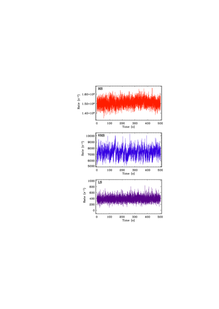
Figure 1: Representative light curves during HS (top panel), VHS (middle panel), and LS (bottom panel). Time bin is 0.1 s

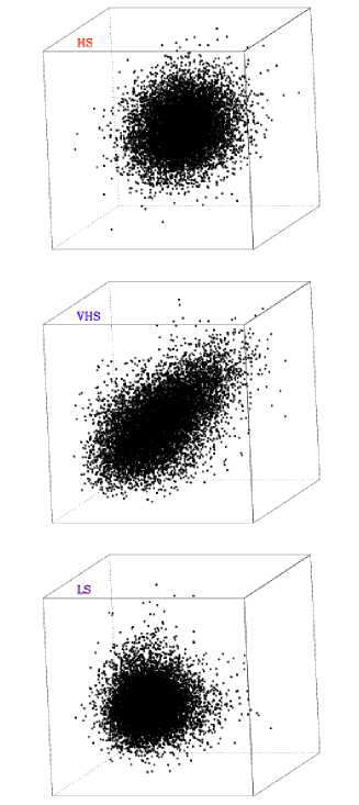
Figure 2: 3-dimensional phase space portraits for HS (top panel), VHS (middle panel), and LS (bottom panel). $\tau=$0.1 s was used for the time-delay reconstruction.

1. As all timing techniques, the very first step starts with a time series. Figure 1 shows three samples of light curves characterizing HS (top panel), VHS (middle panel), and LS (bottom panel) of 4U 1543–47 during the 2002 outburst. For clarity reasons, 500 s time intervals (i.e., intervals with 5000 data points) are plotted, although the results described in $\S$4.1 are obtained using 1000 s (10,000 points) intervals; the time bin used for all light curves is 0.1 s. Before applying the SIM, the light curves are normalized, in the sense that the mean count rate is subtracted from each data point and the resulting quantity is divided by the total standard deviation. In any variability analysis, particular attention should be paid to low count rate intervals due to the Poisson noise that may swamp the signal and hamper the analysis. Despite the large difference in count rate and hence in Poisson noise (during the 2002 outburst the average RXTE PCA count rate during individual observations ranges between $\sim$18,000–400 count/s), the SIM analysis appears to be largely unaffected by the actual count rate (see $\S$4.2 for more details).

2. As most of the methods of nonlinear dynamics applied to timing analysis, the SIM relies upon the phase space reconstruction, which is obtained via the time-delay reconstruction (e.g., Kantz, & Schreiber 1997; Regev 2006). In simple words, in the case of a 3-dimensional (3-D) phase space reconstruction, one constructs a set of 3-D vectors by selecting triplets of data points from the original time series, which are separated in time by the time-delay $\tau$. More specifically, the second data-point (which represents the y-component in a 3-D vector) is separated from the first one (the x-component) by a time delay of $\tau$, whereas the third data-point (the z-component) is separated from the first one by 2 $\tau$, and from the second one by $\tau$. Figure 2 illustrates the phase space portraits in 3 different spectral states, i.e. the results of a 3-D phase space reconstruction for the light curves shown in Figure 1 using a time delay of $\tau=0.1$ s. Not surprisingly, just like the light curve plotted in the middle panel of Fig. 1 looks different from the other two, the phase space portrait of the VHS looks considerably different from those describing HS and LS. This reflects the fact that, unlike HS and LS, the VHS light curve is characterized by the presence of frequent peaks and dips in a quasi-periodic fashion, which increase the degree of correlation observed in the phase space reconstruction.

3. After the phase space reconstruction, the temporal properties of the original time series translate into topological properties of the phase space portraits. In order to quantify these topological properties, a useful method is based on the measure of the crowding around each individual vector. This measurement is formally performed by computing the cumulative number function, $C_{i}(R)=n\{j|d_{ij}\leq R\}$, which measures the number of vectors $j$, whose distance $d_{ij}$ from a vector $i$ is smaller than $R$. Generally, when plotted versus $R$ in log-log space, the function $C_{i}(R)$ can be approximated by a power law, $C_{i}(R)\propto R^{\alpha_{i}}$, for a wide range of values of $R$. The exponent, $\alpha_{i}=[\log(C_{i}(R_{2}))-\log(C_{i}(R_{1}))]/[\log(R_{2})-\log(R_{1})]$, which is the logarithmic derivative of the cumulative number function, is the scaling index. In summary, for a light curve with $N$ data points and an embedding space of dimension $D$ this process yields $N-D$ values of $\alpha_{i}$. The temporal properties of the original light curve can then be studied either using the distribution of $\alpha_{i}$ or the mean value of this distribution $\langle\alpha\rangle$, as explained in $\S$4.

4. The main difference between “normal” and weighted scaling index methods is that in the latter the cumulative number function is substituted by the weighted cumulative point distribution, where the weighting function can be any differentiable function (in our case a Gaussian function; see Räth et al. 2007 for a detailed explanation of the WSIM). The chief advantage of WSIM is twofold: 1) the logarithmic derivative (i.e., the scaling index) can be computed analytically instead of numerically; 2) the number of free parameters is reduced by 1: since the logarithmic derivative is computed analytically, we only need to define one value $R$ at which it is computed, instead of $R_{1}$ and $R_{2}$.

To summarize, i) we start from normalized light curves, ii) transform them into phase space portraits via time-delay reconstruction, and iii) quantify their differences by computing the weighted scaling index.

Importantly, the mean value $\langle\alpha\rangle$ provides direct information on the nature of the variability process: for a purely random process $\langle\alpha\rangle$ tends to the value of the dimension of the embedding space (i.e., the space used in the phase space reconstruction) , whereas for correlated (and deterministic) processes $\langle\alpha\rangle$ is always smaller than the dimension, $D$, of the embedding space and, in the ideal case where the random component is completely negligible, the mean scaling index is independent of the embedding dimension. In other words, low values of $\langle\alpha\rangle$ characterize correlated variability processes, whereas higher values correspond to variability properties with a higher degree of “randomness”.

Before discussing the results of the WSIM, it is important to understand the role played by the 3 free parameters involved in this process and their impact on the results. The process leading to the phase space reconstruction requires to choose 2 parameters, the time delay $\tau$ and the embedding dimension $D$, and the computation of the weighted scaling index requires an additional parameter, the radius $R$ at which the logarithmic derivative is computed.

A common choice for $\tau$ is the characteristic timescale of the system, which can be determined with different methods (e.g., autocorrelation function, PSD, or the so-called mutual information; Fraser & Swinney 1986). In our analysis we will use $\tau=0.1$ s, which is where the PSDs of 4U 1543–47 show prominent QPOs in the VHS and LS, whereas as expected the PSD of the HS is featureless (see Park et al. 2004). On the other hand, there are no systematic prescriptions for the choice of $D$ and $R$. The latter likely depends on the typical distances (in the following we will use the Euclidean norm as measure of the distance) between vectors, which, in turn, depend on the choice of the embedding space dimension.

In principle, the discriminating power of the SIM is enhanced by using high embedding dimensions. However, for our purposes, a relatively low embedding dimension is preferable, since we work with a limited number of points and since one of our goals is to compare the GBHs variability results with those of AGN, which have light curves characterized by fewer data points than GBHs. Specifically, for our analysis we utilize $D=3$. Once $\tau$ and $D$ are fixed, $R$ is obtained in the following way: first, the temporal order of the data points in the original time series is randomized creating 10 sets of randomized data; second, the mean WSI is computed for randomized and original data using different values of $R$ (specifically between 0.5 and 2.5); finally, the chosen radius (in our case $R=1.6$) is the value that yields the larger difference between randomized data and original data, indicating that it is the value most sensitive to the temporal structure of the original data.

Our nonlinear analysis of the variability properties of 4U 1543–47 is therefore carried out using $\tau=0.1$ s, $D=3$, and $R=1.6$. However, for the sake of completeness, we have performed an investigation of a broad parameter space encompassing $\tau=0.1-10$ s, $D=2-4$, $R=0.6-2.4$. The results of this analysis, which demonstrates that our main findings are largely insensitive to the choice of these 3 parameters, are reported in the Appendix.

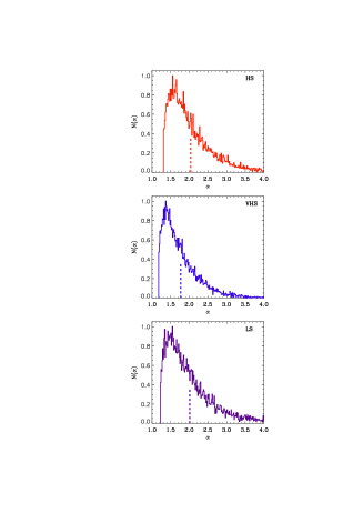
Figure 3: Histograms of the weighted scaling indices (WSIs) for HS (top panel), VHS (middle panel), and LS (bottom panel). The dashed lines represent the mean values. All WSI values were computed for a 3-D embedding space, $\tau=$0.1, and $R=1.6$, using light curves containing 10,000 data points.

4 WSIM Results

As explained before, the temporal properties of a variable system can be studied either via the distribution of the $\alpha_{i}$ values or simply through the mean value $\langle\alpha\rangle$. In the following we elucidate these 2 approaches, by applying the WSIM first to the 3 representative light curves shown in Figure 1, and then to all light curves covering the 2002 outburst of 4U 1543–47.

4.1 WSIM distribution

Given that each of the representative light curve has 10,000 points each and given that the WSIM is applied to each individual vector, this analysis yields nearly 10,000 values of $\alpha_{i}$. The results of this process are illustrated in Figure 3 which shows the $\alpha_{i}$ distributions for the HS (top panel), VHS (middle panel), and LS (bottom panel); the dashed lines represent the mean value $\langle\alpha\rangle$ in the 3 different spectral states.

At first order, all 3 histograms share a similar asymmetric shape with a sharp cut-off on the left-hand side and a broad right-hand tail. The left-hand side of the $\alpha_{i}$ distribution is generally related to the correlated variability component, whereas the right-hand side is related to the random noise component. As a consequence, a highly correlated process is characterized by a narrow $\alpha_{i}$ distribution peaking at low values. On the other hand, a process dominated by random noise will be associated to a broad $\alpha_{i}$ histogram with a pronounced right-hand tail extending to large values of $\alpha$.

A first simple way to assess the difference between the 3 representative histograms is to compare their respective means. For the HS, VHS, and LS we get respectively $\langle\alpha\rangle=2.038\pm 0.006,\leavevmode\nobreak\ 1.769\pm 0.005,\leavevmode\nobreak\ 2.013\pm 0.007$ (where the quoted uncertainties are $\sigma/\sqrt{n}$). These values suggest that the VHS is significantly different from both the HS (at $\sim 33\sigma$ level) and the LS (28 $\sigma$ level), whereas the difference between HS and LS is only marginally significant according to this test (2.7$\sigma$).

A formal comparison between the 3 distributions based on a Kolmogorov-Smirnov test (hereafter K-S test), which is sensitive to the whole distributions of $\alpha_{i}$ suggests that the three distributions are statistically different from each other. Specifically, the K-S test yields a statistic of 0.22 and an associated probability $P_{\rm K-S}<10^{-25}$ that HS and VHS $\alpha_{i}$ histograms are drawn from the same distribution. Similarly, for HS vs. LS and VHS vs. LS we obtain 0.07 ($P_{\rm K-S}\simeq 10^{-24}$) and 0.16 ($P_{\rm K-S}<10^{-25}$), respectively. However, it must be kept in mind that the K-S test is devised for independent data-points, whereas the different $\alpha_{i}$ are not completely independent. As a consequence, the apparently highly significant difference between the 3 histograms representing 3 different spectral states should be considered with caution and need to be confirmed with further analysis (see below).

The results from the histogram analysis are encouraging and suggest that the WSIM has indeed the potential to discriminate between the different spectral states of 4U 1543–47, in full agreement with results from the PSD analysis. However, in order to reach a stronger conclusion, we should demonstrate that all $\alpha_{i}$ histograms of HS are indistinguishable from each other, but statistically different from all the VHS and LS $\alpha_{i}$ histograms. Although feasible, this procedure would be very time consuming and would go against the primary goal of this work, which is to provide a simple alternative way to characterize the temporal properties of GBHs. In addition, it must be pointed out that these results have been obtained using 10,000-point light curves, which are generally not commensurable with typical AGN light curves. This approach would therefore hamper a direct comparison between GBH and AGN, which is one of the secondary goals of this work.

4.2 WSIM mean

Since our primary goal is to define a simple way to characterize the global variability properties of GBHs and since in this kind of analysis the mean value $\langle\alpha\rangle$ is the most robust indicator of the global variability properties, we will restrict our analysis to $\langle\alpha\rangle$. In this way, the properties of a given light curve are defined by a single number, $\langle\alpha\rangle$, in a similar way as the photon index is often used to characterize the energy spectral properties of X-ray sources.

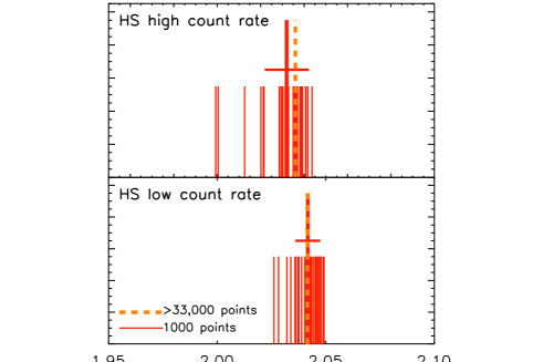
Figure 4: Comparison between the mean scaling index obtained using long light curves ($>$ 33,000 points; thick pale-colored dashed lines) and the values derived using intervals with 1000 points (smaller dark solid lines), whose average is represented by the thick solid lines with horizontal lines indicating the dispersion $\sigma$ . The top panel refers to a high count rate HS ($\sim$16,000 counts/s), whereas the bottom panel describes results from a low count rate HS ($\sim$800 counts/s). All values of $\langle\alpha\rangle$ were computed for a 3-D embedding space, $\tau=$0.1, and $R=1.6$

4.2.1 Test with short intervals

In addition, in order to further generalize this procedure extending it to relatively short light curves, which are more common than long uninterrupted ones, we will use intervals of 100 s (i.e., time series containing 1000 points since the bin time is 0.1 s). In this way, the light curves will contain a number of points comparable to typical AGN light curves, offering the possibility of a direct comparison between GBH and AGN variability properties

Before proceeding further, we must first demonstrate that the choice of shorter intervals will not hamper our analysis. On one hand, from the PSD analysis of Park et al. (2004) we are ensured that nothing relevant occurs to the timing properties of 4U 1543–47 for timescales longer than $\sim$ 100 s: all the interesting PSD features (frequency breaks and QPOs) are located at frequencies well above $10^{-2}$ Hz. On the other hand, we must still verify that the WSIM results are not significantly affected by the use of shorter intervals.

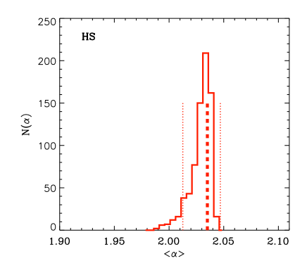
Figure 5: Distribution of the mean WSI values, obtained using segments of 100 s (1000 points) during HS (741 segments). All values of $\langle\alpha\rangle$ were computed for a 3-D embedding space, $\tau=$0.1, and $R=1.6$. The thick dashed line indicates the mean of the $\langle\alpha\rangle$ distribution and the dotted lines represent the 90th percentiles.

To this aim, and to demonstrate that the WSIM is also independent of the mean count rate (and hence of the Poisson noise level), we have performed the following experiment. We have chosen 2 of the longest HS light curves (both have more than 33,000 data points) with mean count rate greatly different: the first light curve, obtained close to the outburst peak, has an average RXTE PCA count rate of $\sim$16,000 counts/s, whereas the second one (corresponding to a later phase of the decay) has a count rate of only $\sim$800 counts/s. We have applied the WSIM to both data sets, first using the entire light curve and then using intervals of 1000 points only. The results are illustrated in Figure 4, where the value of $\langle\alpha\rangle_{33,000}$ for the entire light curve is represented by the thick dashed line, the individual values obtained with 1000 points, $\langle\alpha\rangle_{1000}$, are depicted as shorter continuous lines, and their average is indicated by the thick continuous line. The horizontal lines indicate the standard deviation, $\sigma_{\langle\alpha\rangle_{1000}}$, of the sample of $\langle\alpha\rangle_{1000}$. Figure 4 reveals that:
1) In both cases, $\langle\alpha\rangle_{1000}$ values narrowly cluster around the mean scaling index, $\langle\alpha\rangle_{33,000}$, obtained from the entire light curve and their average, $\langle\langle\alpha\rangle_{1000}\rangle$, is fully consistent with $\langle\alpha\rangle_{33,000}$. This is formally demonstrated by the fact that $|\langle\alpha\rangle_{33,000}-\langle\langle\alpha\rangle_{1000}\rangle|/(\sigma_{\langle\alpha\rangle_{1000}}/\sqrt{n})=2.5$ (for the high count rate case) and 0.1 (for the low count rate case), which are both lower than the 3$\sigma$ level. This indicates that WSIM results obtained with 100 s intervals are fully consistent with those obtained using a longer interval. Therefore, with this method the variability properties of 4U 1543–47 can be thoroughly investigated using 100 s intervals.
2) Although visually the high and low count rate distributions of $\langle\alpha\rangle_{1000}$ and their respective mean look fairly close and indeed their standard deviations significantly overlap, statistically speaking, their difference $|\langle\langle\alpha\rangle_{\rm 1000,high}\rangle-\langle\langle\alpha\rangle_{\rm 1000,low}\rangle|$ is slightly above the formal 3$\sigma$ level. In order to thoroughly address this issue, and estimate quantitatively the uncertainty on the scaling index during the HS, we need to account for all the observations during HS. This is illustrated in Figure 5, which shows the distribution of $\langle\alpha\rangle_{1000}$ obtained using all the 100 s intervals of all the available HS observations. Despite the huge difference in count rate (max$>$ 18,000 counts/s, min$<$370 counts/s) and a temporal separation longer than 30 days, the vast majority of values narrowly clusters around the mean, yielding $\langle\langle\alpha\rangle_{\rm 1000}\rangle=2.035_{-0.022}^{+0.012}$, where the quoted uncertainties are the 90th percentiles (the error on the mean is $\sigma/\sqrt{n}=0.01/\sqrt{741}=0.0004$). The “narrowness” of the distribution of the $\langle\alpha\rangle$ values shown in Fig. 5, really suggests that WSIM results are not affected neither by the fact that the light curves have vastly different signal-to-noise ratios nor by the time span over which the HS light curves are spaced. It is therefore suggestive that $\langle\alpha\rangle$ is most probably determined just by one factor, i.e. the properties of the variability mechanism during the HS.

For completeness, we also carried the previous test for the two VHS and LS light curves. Note that the short duration of the VHS (due to the intrinsic transient behavior of this short-lived state) and the LS (due to the interruption in the PCA monitoring program) yielded only 2 light curves for each state. In both cases, $\langle\langle\alpha\rangle_{1000}\rangle\rangle$ is fully consistent with $\langle\alpha\rangle_{\rm whole}$, as their difference is of the order of 1 $\sigma$ or less. Similarly, the values of the difference between the pair of light curves corresponding to the same state, $|\langle\langle\alpha\rangle_{\rm 1000,A}\rangle-\langle\langle\alpha\rangle_{\rm 1000,B}\rangle|/\sqrt{\sigma_{\rm A}^{2}+\sigma_{\rm B}^{2}}$, is 0.07 and 1.4 for the VHS and LS, respectively.

4.2.2 Discrimination of spectral states

We can now assess whether the WSIM is able to discriminate between the spectral different states, by considering all the available observations, dividing all the individual light curves covering the 2002 outburst into 100 s intervals and treating each segment as an independent data-set. This procedure yields 741 data sets for HS, 31 for VHS, and 40 for LS.

Figure 6 shows the normalized distribution of $\langle\alpha\rangle_{1000}$ values for the HS (dotted line), LS (solid line), and VHS (dashed line), as well as their average of the mean WSIs. The HS and LS distributions are very narrow, and they appear to be offset, with the LS values of $\langle\alpha\rangle$ being systematically lower than the respective values of HS. The VHS distribution has a rather large width, but is this mainly due to the fact that, in addition to the 2 VHS observations, we also included here the data from the observation just before the source entered fully the VHS state, which caught the source during a transition phase (see $\S$4.3). In any case though, the VHS values of $\langle\alpha\rangle$ appear to be systematically much lower than the values in the LS and/or HS.

A simple and robust way to quantify the difference between the 3 different states is to compare their respective means by computing the quantity $\Delta\alpha_{\rm A-B}\equiv|\langle\alpha_{\rm A}\rangle-\langle\alpha_{\rm B}\rangle|/\sqrt{\sigma_{\rm A}^{2}+\sigma_{\rm B}^{2}}$, where $\langle\alpha_{\rm A}\rangle$ is the mean scaling index obtained using all the 100 s intervals during the spectral state $A$ , and $\sigma^{2}_{\rm A}$ is the variance divided by the number of 100 s intervals in that state. This test yields respectively $\Delta\alpha_{\rm VHS-HS}=8.4$, $\Delta\alpha_{\rm VHS-LS}=7.2$, and $\Delta\alpha_{\rm HS-LS}=10.3$, indicating that the WSIM is indeed able to statistically discriminate between the 3 states.

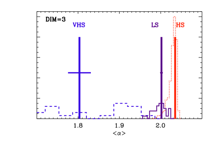
Figure 6: Normalized distributions and averages of mean WSIs for HS, VHS, and LS, obtained using segments of 100 s (1000 points) from all the available light curves. The uncertainties shown represent the error on the mean (i.e., $\sigma/\sqrt{n}$, where $n$ is the number of data sets); for HS the uncertainty is smaller than the thickness of the vertical bar representing the mean. All values were computed for a 3-D embedding space, $\tau=$0.1, and $R=1.6$. The maximum of the HS histogram has been normalized to 1, whereas the VHS and LS have been normalized to 0.15, only for clarity reasons. No visual comparison would have been possible maintaining the real proportions between the distributions, given that VHS and LS only contain 30–40 data-points as opposed to the 741 contained in the HS

.

The significance of the difference between the WSIs in the three spectral states can also be examined using a K-S test, which can be safely applied to the 3 distributions of $\langle\alpha_{i}\rangle$, since each data-point has been obtained from a separate 100 s interval, which in many cases are separated by a few days intervals, and hence can be considered as being independent “measurements”. Specifically, the K-S test yields 0.93 ($P_{\rm KS}<8\times 10^{-24}$), 0.78 ($P_{\rm KS}<2\times 10^{-10}$), and 0.75 ($P_{\rm KS}<6\times 10^{-20}$), for the cases of VHS vs. HS, VHS vs. LS, and VHS vs. LS.

In summary, the main results of the analysis based on all available light curves divided into 100 s intervals can be summarized as follows:
1) In all 3 spectral states $\langle\alpha\rangle<D$ (where $D=3$ is the embedding space dimension). This result implies the presence of correlated variability, which is expected given the red-noise trend observed in all PSDs.
2) The 3 spectral states have different mean scaling indices satisfying the following relationship: $\langle\alpha\rangle_{\rm VHS}\leavevmode\nobreak\ <\leavevmode\nobreak\ \langle\alpha\rangle_{\rm LS}\leavevmode\nobreak\ <\langle\alpha\rangle_{\rm HS}$. In addition to formally demonstrating that the scaling index method is able to discriminate between the spectral states of 4U 1543–47, this results indicates that the VHS is the state characterized by the highest degree of correlated variability. Also this result is somewhat expected from the linear temporal analysis, given the presence of a prominent QPO in the VHS PSD. However, the low value of $\langle\alpha\rangle_{\rm VHS}$ might also be related to non-linear correlations, i.e., any temporal correlations that cannot be detected by the PSD or autocorrelation function and that manifest themselves as correlation in the Fourier phases. This will be discussed in more detail in $\S 5$.

4.3 Temporal evolution of $\langle\alpha\rangle$

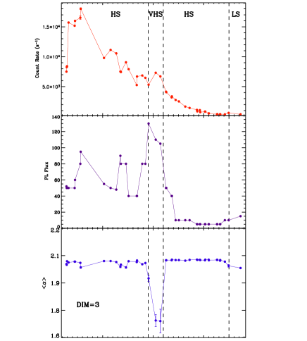
Figure 7: Temporal evolution during the 2002 flare of 4U 1543–47 for the RXTE PCA count rate (top panel), flux associated with the PL component in units of $10^{-10}\leavevmode\nobreak\ {\rm erg\leavevmode\nobreak\ cm^{-2}\leavevmode\nobreak\ s^{-1}}$ (middle panel), and mean WSIM (bottom panel). The statistical errors are in most cases smaller than the symbols.

After having demonstrated that the WSIM is a reliable tool to characterize the variability properties in different spectral states, we focus now on the temporal evolution of the mean scaling index during the 2002 flare of 4U 1543–47. Since the source spends the vast majority of the time in the thermal dominated HS, no substantial changes in the energy spectral parameters appear to occur during the outburst (see Fig. 3 of Park et al. 2004). On one hand, this spectral behavior represents a considerable advantage to thoroughly assess the uncertainty on $\langle\alpha\rangle$, but on the other hand it partially hampers a detailed study of correlated spectral and temporal variability. Nevertheless, it is interesting to investigate if (and how) the changes of $\langle\alpha\rangle$ are related to the flux changes during the outburst evolution. The results of this analysis are illustrated in Figure 7: the top panel describes the temporal evolution of the total count rate that is roughly proportional to the evolution of disk flux and color temperature; the middle panel shows the flux associated with the power law component in units of $10^{-10}\leavevmode\nobreak\ {\rm erg\leavevmode\nobreak\ cm^{-2}\leavevmode\nobreak\ s^{-1}}$, which was derived from Fig. 2 of Park et al. (2004); finally, the bottom panel presents the $\langle\alpha\rangle$ temporal evolution. The scaling index analysis is carried out dividing each individual observation into intervals of 100 s, computing $\langle\alpha\rangle$ for each interval, and then taking the mean over all intervals belonging to a given observation. The error-bars for the mean scaling indices are given $\sigma/\sqrt{n}$ (where $n$ is the number of 100 s intervals of a given observation), which are often smaller than the symbols shown in the bottom panel of Fig. 7.

The temporal trend of $\langle\alpha\rangle$ can be summarized as follows: the mean scaling index remains roughly constant around 2.05 for the whole duration of the outburst, with the notable exception of a deep dip during the VHS state. A closer look at Fig. 7 reveals 2 minor dips preceding the VHS and a steady decrease toward the end of the outburst when the source is entering the LS. Interestingly, while these changes of $\langle\alpha\rangle$ appear to be uncorrelated with the overall count rate (and hence with the disk flux), they seem to occur in correspondence of local maxima in the power law flux. At zeroth order, such apparent correlation can be interpreted in the following way: the variability associated with the power law component is “less random” than the one produced by the disk. However, additional data and a systematic analysis of correlated spectral and temporal properties is necessary before drawing firmer conclusions.

Perhaps the most remarkable result from Fig. 7 is the fact that after $\sim$MJD 52462, while both the PL flux and the total count rate decrease very significantly (in an abrupt way the PL flux and in a smoother way the disk flux), $\langle\alpha\rangle$ returns to the same level it was before the VHS state. In other words, $\langle\alpha\rangle$ appears to be a true indicator of state, as it is defined based on spectral and timing criteria.

5 Search for Nonlinearity

The second goal of this work is to search for nonlinear temporal correlations in the variability properties of 4U 1543–47. Investigating the nature of the temporal variations is of primary interest for constraining models of variability in GBHs (and AGN). Indeed, unlike the results from the PSD and auto-correlation analyses, which can be equally well explained by a variety of different physical models, the detection of nonlinear variability would immediately rule out any intrinsically linear model that explain the X-ray variability as the superposition of many independent active regions (e.g., Terrel 1972). Therefore, this analysis has the potential to provide model-independent constraints that will break the current model degeneracy.

In order to find out whether a time series can be completely modeled by superimposed linear processes (plus uncorrelated noise) or whether signatures of nonlinear correlations are present, one of the most direct approaches is based on the idea of surrogate data sets introduced by Theiler et al. (1992; see Kantz, & Schreiber 1997 for a review). In simple words, this technique can be summarized as follows:
1) Assume as null hypothesis that the original time series is linear.
2) Construct linear surrogate data that have the same linear characteristics of the original data. In other words, the PSD of surrogate data should be indistinguishable from that of the original data, since linear processes are by definition completely characterized by the PSD or alternatively by the autocorrelation function.
3) Use an appropriate nonlinear statistic to test the null hypothesis comparing original and surrogate data. If this test yields consistent values for surrogates and real data, we conclude that the original time series is linear in nature. On the other hand, if the value of the nonlinear statistic for the real data is significantly different from the corresponding values obtained using surrogates, then we infer the presence of nonlinearity.

Before presenting the results from this test, it is instructive to describe a few basic details of the technique used to create surrogate data and the main characteristics of the nonlinear statistic used in this case.

The most popular algorithms used to generate an ensemble of surrogate realizations are the Amplitude Adjusted Fourier Transform (AAFT) and the Iterative Amplitude Adjusted Fourier Transform (IAAFT) algorithms (Theiler et al. 1992; Schreiber & Schmitz 1996). Although the AAFT and IAAFT algorithms conserve the amplitude distribution in real space and reproduce the PSD of the original data set quite accurately, it has been shown recently that both algorithms may induce unwanted correlations in the Fourier phases (Räth & Monetti 2008). To guarantee that the surrogates in this study are free from any higher order correlations, we generate them in the following way: First, the time series is mapped onto a Gaussian distribution in a rank-ordered way, which means that the amplitude distribution of the original times series in real space is replaced by a Gaussian distribution in such a way that the rank-ordering is preserved, i.e. the lowest value of the original distribution is replaced with the lowest value of the Gaussian distribution etc. By applying this remapping we automatically focus on the temporal correlations of the data, while excluding any contributions to nonlinear correlations stemming from the non-Gaussianity of the original intensity distribution. Second, we Fourier transform the remapped time series, replace the original phases by a new set of uniformly distributed and uncorrelated phases and perform an inverse Fourier transformation. Note that the surrogate time series generated in such a way preserve exactly the power spectrum, while explicitly controlling the randomness of the phases. For each time series under study we generate $50$ corresponding surrogates.

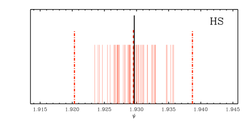
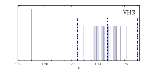
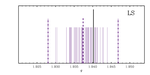
Figure 8: Nonlinear prediction error (NLPE) for the HS (top panel), VHS (middle panel), and LS (bottom panel). The black lines show the NLPE for the original time series. The smaller thin colored lines denote $\psi$ for the respective surrogates. The thicker and longer dashed line indicate the mean value $\langle\psi\rangle$ as derived from the 50 surrogate realizations. The dash-dotted lines mark the $3\sigma_{\psi}$ interval, i.e. $\langle\psi\rangle-3\sigma_{\psi}$ and $\langle\psi\rangle+3\sigma_{\psi}$, where the standard deviation $\sigma_{\psi}$ is also derived from the surrogates.

Although in principle any nonlinear statistics may be used to compare real and surrogate data, a systematic study performed by Schreiber & Schmitz (1997) indicates that the nonlinear prediction error (NLPE) is one of the most effective indicators of nonlinearity and has good discrimination power to detect any deviation from a Gaussian linear stochastic process. Therefore, to test the presence of nonlinearity in 4U 1543–47 light curves we make use of the NLPE.

The equation used to compute the NLPE (hereafter $\psi$) as well as some technical details are provided in Appendix B. Here we simply describe in a qualitative way the main characteristics of this nonlinear indicator. Since this method relies on the time delay embedding technique described in $\S 3$, it can exploit the direct correspondence between the scalars of the starting time series, $x_{1},\leavevmode\nobreak\ ,x_{2},\leavevmode\nobreak\ ...,x_{n}$, and the corresponding set of vectors in the pseudo phase space: ${\bf x_{1},\leavevmode\nobreak\ ,x_{2},\leavevmode\nobreak\ ...,x_{n}}$. Specifically, to predict the “future” measurement $x_{n+10}$ (i.e., the value of the time series 10 steps ahead of $x_{n}$), one must find the closest vector to ${\bf x_{n}}$, which we will call ${\bf x_{i}}$ and corresponds to the scalar $x_{i}$, and then use the scalar $x_{i+10}$ as a predictor for $x_{n+10}$. As explained in Appendix B, the rigorous process is slightly more complicated and involves several vectors in the neighborhood of ${\bf x_{n}}$, which in turn will yield several predictors. The nonlinear prediction error $\psi$ is then provided by the average of the differences between the actual value $x_{n+10}$ and the different predictor values.

We have carried out this test for all the light curves relative to the 2002 outburst of 4U 1543–47, although for clarity reasons in Figure 8 we only show the results for the 3 representative light curves of the HS, VHS, and LS introduced in $\S$3. From this figure, it is clear that the absolute values of $\psi$ for the HS and IS are considerably larger than those measured in the VHS. This is an expected behavior, because in the VHS the time series is much more correlated with linear components showing up as QPO. As a consequence, its predictability increases leading to lower values of $\psi$. More importantly, Figure 8 reveals that the VHS shows highly significant signatures for nonlinear correlations, unlike the HS and IS for which the values of $\psi$ obtained using real data are fully consistent with the values derived using linear surrogates.

Analyzing all time series belonging to the different spectral states we infer that all the HS and LS light curves are linear, whereas the 2 VHS light curves show respectively highly significant and marginally significant signs of nonlinearity. Specifically, the time series on MJD=52461, which corresponds to the absolute minimum of the scaling index, shows the strongest and the only statistically significant evidence ($\sim 7.5\sigma$) for nonlinearity, as illustrated by the middle panel of Figure 8. A day before, on MJD=52460, the evidence of nonlinearity is marginal (at a $\sim 2.4\sigma$ significance level). Finally, the light curve on MJD=52459 that caught 4U 1543–47 during the HS-to-VHS transition (see Fig. 7) shows no indications of nonlinearity at all.

In conclusion, the surrogate test reveals that: 1) All HS and LS light curves are linear, 2) non-linearity indications appear during the VHS light curves, and the highest and most significant signal for non-linearity occurs for this light curves with the strongest QPO and the lowest value of $\langle\alpha\rangle$. On one hand, the latter result suggests that the physical mechanism leading to strong QPOs is intrinsically nonlinear, implicitly disfavoring QPO linear models. On the other hand, it indicates that the low value of $\langle\alpha\rangle$ measured in the VHS is at least partially related to the presence of nonlinear correlations, which cannot be detected by linear timing techniques.

6 Summary and Conclusions

We have carried out a nonlinear analysis of the variability properties of the X-ray nova GBH 4U 1543–47. The main results can be summarized as follows:

• We have used the WSIM to assign a single number, the mean scaling index $\langle\alpha\rangle$, to each individual light curve of the source. The large number of data when the source was in its HS, showed that the resulting $\langle\alpha\rangle$ values remain roughly constant, irrespective of large changes in flux associated to the disk and PL components.

• Similarly, the mean scaling index values remained roughly constant during the VHS and LS, showing the following relationship: $\langle\alpha\rangle_{\rm VHS}\leavevmode\nobreak\ <\leavevmode\nobreak\ \langle\alpha\rangle_{\rm LS}\leavevmode\nobreak\ <\langle\alpha\rangle_{\rm HS}$. These results, which need to be confirmed for other GBHs, suggest that the mean scaling index $\langle\alpha\rangle$ may be used to parametrize the timing properties of an accreting source, and that it may be a true indicator of “state” in these systems.

• When plotted versus time, the $\langle\alpha\rangle$ trend shows no direct correlation with the total flux temporal behavior, which is dominated by the accretion disk emission. On the other hand, the temporal evolution of $\langle\alpha\rangle$ appears to be somewhat related to that of the power-law spectral component: $\langle\alpha\rangle$ reaches its absolute minimum roughly at the same time as the PL flux reaches its absolute maximum, which occurs during the VHS state.

• The search for nonlinearity using surrogate data and NLPE reveals that the variability is linear in all light curves with the notable exception of one observation in the VHS, which corresponds to the absolute minimum of $\langle\alpha\rangle$ and is also characterized by the presence of a strong QPO.

An important implication of the detection of nonlinearity in the VHS is that all intrinsically linear models proposed to produced low frequency QPOs (LFQPOs) may be ruled out for 4U 1543–47. The formation of QPOs (at both high and low frequencies) in GBHs is currently a matter of debate, as several viable competing models have been proposed (see, e.g., McClintock & Remillard 2006 for a review). It is therefore important to derive model-independent constraints that may break or at least reduce the current model degeneracy. If the detection of nonlinearity associated with strong LFQPOs is confirmed in other GBHs, then intrinsically linear models such as the global disk oscillations proposed by Titarchuk & Osherovich (2000) can be safely ruled out, whereas alternative models such as the shock oscillation model (Chakrabarti & Manickam 2000) or the accretion-ejection instability model (Tagger & Pellat 1999), which may account for nonlinearities, are still viable solutions.

In summary, the findings derived from this work suggest that this kind of nonlinear analysis can be useful in the field of GBHs and complement the temporal analysis carried out with linear techniques. Specifically, the simplicity of the WSIM, which characterizes the global variability properties of a light curve via a single number, $\langle\alpha\rangle$, suggests that this technique might be successfully applied to study correlated temporal and spectral variability. In addition, the robustness of the WSIM, that performs well also with noisy data and relatively short light curves, naturally suggests an application to AGN variability with the possibility of direct comparison with GBHs.

Since we have limited our analysis to 4U 1543–47 only, before deriving any general conclusions, we should carry out a systematic nonlinear analysis on several GBHs during their spectral transition. Specifically, it will be important to assess whether specific values of $\langle\alpha\rangle$ are associated with specific spectral states (e.g., $\langle\alpha\rangle_{\rm VHS}\simeq 1.8$, $\langle\alpha\rangle_{\rm HS}\simeq 2.0$, $\langle\alpha\rangle_{\rm HS}\simeq 2.05$), or if only the temporal trend of $\langle\alpha\rangle$ during the outburst (i.e., the presence of a pronounced minimum during the VHS) is similar to the one displayed by 4U 1543–47. To this aim we will carry out a similar analysis on a few prominent GBHs with outbursts that are completely covered by the RXTE PCA and where the different spectral state are well sampled. This test will unequivocally reveal whether $\langle\alpha\rangle$ can be used as reliable indicator of spectral states. In addition, the planned study will provide useful information on correlated variability of $\langle\alpha\rangle$ and several relevant spectral parameters, and on the presence of nonlinearity in different spectral states.

Appendix A Dependence of SIM on $\tau$, $D$, and $R$

As explained in $\S 3$, the WSIM depends on 3 parameters: time delay $\tau$ and embedding dimension $D$, which are related to the phase space reconstruction process, and the radius $R$ at which the logarithmic derivative (i.e., the scaling index) is computed.

In this section, we visually demonstrate that the impact of these parameters on our main findings is basically irrelevant for a broad range of reasonable choices. Figure. 9 shows the temporal evolution of $\langle\alpha\rangle$ for $D=$2 (top panel), 3 (middle panel), and 4 (bottom panel). Solid lines refer to $\tau=0.1$ s, dotted lines to $\tau=1$ s, and dashed lines to $\tau=100$ s; in this case the radius is fixed at 1.6. It is noticeable that all the values of $\langle\alpha\rangle$ consistently increase as the embedding dimension increases. This reflects the fact that a significant part of the variability is random and this random component translates into larger values of $\alpha$ as the dimension of the embedding space increases.

From Fig. 9 it is evident that all different combinations of $\tau$ and $D$ reproduce the same temporal evolution trend of $\langle\alpha\rangle$ with a large central dip preceded by to low-amplitude dips and followed by a final steady decrease. It is also clear that using long time delays, such as $\tau=100$ s, the dips appear less prominent. This simply reflects the fact that long time delays necessarily loose the information relative to short-term temporal correlations.

Figure. 10 illustrates the impact of the radius $R$ on the temporal evolution of $\langle\alpha\rangle$ (this time $D=3$ and $\tau=0.1$ s). Once again, all values of $R$ are able to recover the same temporal evolution trend of $\langle\alpha\rangle$ described above.

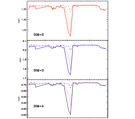
Figure 9: Temporal evolution of the mean WSIM during the 2002 flare of 4U 1543–47 for embedding dimensions 2 (top panel), 3 (middle panel), and 4 (bottom panel). Solid, dotted, and dashed lines refer to $\tau=0.1,\leavevmode\nobreak\ 1$, and 10 s, respectively.

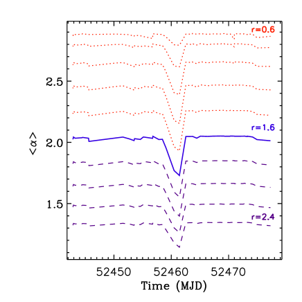
Figure 10: Temporal evolution of the mean WSIM during the 2002 flare of 4U 1543–47 for embedding dimensions 3, with $r$ ranging from 0.6 (top dotted line) to 2.4 (bottom dashed line).

Appendix B Nonlinear Predictor Error

To calculate NLPE, the time series is embedded in a $D$-dimensional space using the method of delay coordinates as described in section 3. We use here also the embedding dimension $D=3$. The delay time $\tau$ was determined using the criterion of zero crossing of the autocorrelation function considering the VHS, where the ACF is sufficiently different from a random process. The NLPE is defined as

$$\psi=\frac{1}{M-T-(D-1)\tau}\left(\sum_{n=(D-1)\tau}^{M-1-T}[\@vec{x}_{n+T}-F(\@vec{x}_{n})]^{2}\right)^{1/2}$$ (1)

where $F$ is a locally constant predictor (i.e., a quantity that remains constant for a local surrounding of a point under study in the D-dimensional embedding space), $M$ is the length of the time series, and $T$ is the lead time (i.e., the number of time steps ahead of the considered one for which we want to make a prediction). The predictor $F$ is calculated by averaging over future values of the $N\,(N=D+1)$ nearest neighbors in the delay coordinate representation. We have studied the behavior of $\psi$ as a function of the lead time $T$ and did not find significant variations. We set this value to $T=10$ time steps. The results of this analysis for the 3 representative light curves of the HS, VHS, and LS are shown in Figure 8.

References

- (1) Atmanspacher, H., Scheingraber & H., Wiedenmann G. 1989, Phys.Rev.A, 40, 3954
- Chakrabarti & Manickam (2000) Chakrabarti, S.K. & Manickam, S.G. 2000, ApJ, 531, L41
- Corbel et al. (2006) Corbel, S., Tomsick, J.A., & Kaaret, P. 2006, ApJ, 636, 971
- D’Angelo et al. (2008) D’Angelo, C., Giannios, D., Dullemond, C., & Spruit, H. 2008, A&A, 488, 441
- Done et al. (2007) Done, C., Gierliński, M., & Kubota, A. 2007, A&ARv, 15, 1
- Fraser & Swinney (1986) Fraser, A.M. & Swinney, H.L. 1986, Phys. Rev.A, 33, 1134
- Fender et al. (2004) Fender, R.P., Belloni, T.M., & Gallo, E. 2004, MNRAS, 355, 1105
- Gierliński et al. (2008) Gierliński, M., Done, C.,& Page, K. 2008, MNRAS, 388, 753
- (9) Gliozzi, M., Brinkmann, W., Räth, C., et al. 2002, A&A, 391, 875
- Gliozzi et al. (2006) Gliozzi M., Papadakis, I.E., & Räth, C. 2006, A&A, 449, 969
- Ivlev et al. (2008) Ivlev, A.V., et al. 2008, PhysRevLett, 100, 095003
- (12) Kantz, H., & Schreiber, T. 1997, Nonlinear Time Series Analysis (Cambridge University Press)
- Klein-Wolt & van der Klis (2008) Klein-Wolt, M. & van der Klis, M. 2008, ApJ, 675, 1407
- Körding et al. (2006) Körding, E.G., Jester, S., & Fender, R. 2006, MNRAS, 372, 1366
- Markoff et al. (2001) Markoff, S., Falcke, H., & Fender, R. 2001, A&A, 372, L25
- McClintock & Remillard (2006) McClintock, J.E. & Remillard R.A. 2006, “Compact Stellar X-ray Sources” ed. W.H.G. Lewin and M. van der Klis, Cambridge University Press, 157 (astro-ph/0306213)
- McHardy et al. (2006) McHardy, I.M., Körding, E., Knigge, C., Uttley, P., & Fender, R.P. 2006, Nature, 444, 730
- (18) Miller, J.M., Homan, J., & Miniutti, G. 2006a, ApJ, 652, L113
- (19) Miller, J.M., et al. 2006, ApJ, 653, 525
- Misra et al. (2004) Misra, R., Harikrishnan, K.P., Mukhopadhyay, B., Ambika, G., & Kembhavi, A.K. 2004, ApJ, 609, 313
- Misra et al. (2006) Misra, R., Harikrishnan, K.P., Ambika, G., & Kembhavi, A.K. 2006, ApJ, 643, 1114
- Morfill & Bunk (2001) Morfill, G.E. & Bunk, W. 2001, Europhysics News, vol. 32, issue 3, 77
- Park et al. (2004) Park, S.Q., et al. 2004, ApJ, 610, 378
- Raeth et al. (2002) Räth, C., et al. 2002, MNRAS, 337, 413
- Raeth et al. (2007) Räth, C., Schuecker, P., & Banday, A.J. 2007, MNRAS, 380, 466
- Raeth et al. (2009) Räth, C., Morfill, G.E., Rossmanith, G., Banday, A.J., & Górski, K.M. 2009, PhysRevLett, 102, 131301
- Raeth & Monetti (2008) Räth, C., & Monetti, R., Surrogates with random Fourier Phases, in: Topics on Chaotic Systems, Selected Papers from CHAOS 2008 International Conference, Edited by C. H. Skiadas, I. Dimotikalis, C. Skiadas, World Scientific Publishing, pp. 274-285 (2009), (http://arxiv.org/abs/0812.2380)
- Regev (2006) Regev, O. 2006, Chaos and Complexity in Astrophysics (Cambridge University Press)
- Reig et al. (2006) Reig, P., Papadakis, I.E., Shrader, C.R., & Kazanas, D. 2006, ApJ, 644, 424
- Schreiber & Schmitz (1996) Schreiber, T. , & Schmitz A. 1996, Phys. Rev. Lett., 77, 635
- Schreiber & Schmitz (1997) Schreiber, T. , & Schmitz A. 1997, Phys. Rev. E., 55(5), 5443
- Sugihara & May (1990) Sugihara, G., & May, R. 1990, Nature, 334, 734
- Sütterlin et al. (2009) Sütterlin, K.R., et al. 2009, PhysRevLett, 102, 085003
- Tagger & Pellat (1999) Tagger, M. & Pellat, R. 1999, A&A, 349, 1003
- Terrel (1972) Terrel, N.J. 1972, ApJ, 174, L35
- Theiler et al. (1992) Theiler, J., et al. 1992, Physica D, 58, 77
- Titarchuk & Osherovich (2000) Titarchuk, L. & Osherovich, V. 2000, ApJ, 542, L111
- Tomsick et al. (2004) Tomsick, J.A., Kalemci, E., & Kaaret, P. 2004, ApJ, 601, 439
- Zdziarski et al. (2003) Zdziarski, A.A., Lubiǹski, P., Gilfanov, M & Revnivtsev, M. 2003, MNRAS, 342, 355