CP Violating Asymmetry in Stop Decay into Bottom and Chargino

Abstract

In the MSSM with complex parameters, loop corrections to the decay of a stop into a bottom quark and a chargino can lead to a CP violating decay rate asymmetry. We calculate this asymmetry at full one-loop level and perform a detailed numerical study, analyzing the dependence on the parameters and complex phases involved. If the stop can decay into a gluino, the self-energy and the vertex correction dominate due to the strong coupling. It is shown that the vertex contribution is always suppressed. We therefore give a simple approximate formula for the asymmetry. We account for the constraints on the parameters coming from several experimental limits. Asymmetries up to 25 percent are obtained. We also comment on the feasibility of measuring this asymmetry at the LHC.

1 Introduction

If the Minimal Supersymmetric Standard Model (MSSM) is realized in nature, LHC will produce squarks and gluinos copiously. However, even if supersymmetry is discovered, it will be still a long way to determine the parameters of the underlying model. In the general MSSM, the U(1), SU(2) and SU(3) gaugino mass parameters $M_{1}$, $M_{2}$, and $M_{3}$, the higgsino mass parameter $\mu$, and the trilinear couplings $A_{f}$ (corresponding to a fermion f) may be complex, i.e. $A_{f}=|A_{f}|e^{i\varphi_{A_{f}}}$, $M_{3}=|M_{3}|e^{i\varphi_{\tilde{g}}}$. As usual, we take $M_{2}$ positive and real by field redefinition Dugan:1984qf . The experimental upper bounds on the electric dipole moment (EDM) of the electron, muon, neutron and several atoms severely constrain the phase of $\mu$. In general, the phases of $M_{1}$, $M_{3}$ and $A_{t,b}$ are much weaker constrained due to possible cancelations Ibrahim:1997gj ; Brhlik:1998zn ; Bartl:1999bc ; Pilaftsis:2002fe ; Bartl:2003ju ; Barger:2001nu ; Pospelov:2005pr ; Olive:2005ru ; Abel:2005er ; YaserAyazi:2006zw ; Ellis:2008zy . Therefore, we use real values only for $\mu$ and do not restrict the remaining phases. (For a recent discussion on EDMs see Gajdosik:2009sd .)

Complex MSSM parameters can lead to direct CP violation (CPV), see the summary in Kraml:2007pr . One example is the CP violating rate asymmetry, which is a loop induced effect. CP violating asymmetries for the production and decays of the charged Higgs $H^{\pm}$ Christova:2002ke ; Christova:2006fb ; Christova:2002sw ; Christova:2003hg ; Ginina:2008xa ; Christova:2008bd ; Christova:2008jv ; Frank:2007zza ; Frank:2007ca ; Arhrib:2007rm and for the decays $\tilde{\chi}^{\pm}\to W^{\pm}\tilde{\chi}^{0}$ Eberl:2005ay were already studied in detail. Studies of measuring direct CP violation in stop cascade decays at the LHC based on T-odd asymmetries built from triple products were done in Ellis:2008hq ; Deppisch:2009nj ; MoortgatPick:2009jy .

In the following, we study the CP violating decay rate asymmetry of the decays $\tilde{t}_{i}\to b\,\tilde{\chi}^{+}_{k}$ and $\tilde{t}_{i}^{*}\to\bar{b}\,\tilde{\chi}^{-}_{k}$ at full one-loop level Frank:2009re ; Frank2008 . If the channel $\tilde{t}_{i}\to\tilde{g}\,t$ is kinematically open, the $\tilde{t}_{1}-\tilde{t}_{2}$ self-energy and the vertex graph with $\tilde{g}$ exchange are expected to dominate because of the strong coupling. But we show explicitly that the vertex contribution is suppressed. All other contributions are numerically always smaller than $\sim\!0.5\%$ which also means that the dependence on the phase of $M_{1}$ is negligible. We thus give a short analytic formula for the decay rate asymmetry $\delta^{CP}$ which approximates the total one-loop result within $5\%$ in the range above the threshold of the $\tilde{t}_{i}\to\tilde{g}\,t$ decay.

In order to get a large decay rate asymmetry, not only the channel into $\tilde{g}$ must be open, but also large phases or phase combinations of $A_{t}$ and $M_{3}$ are necessary. In addition, the stops must be rather degenerate but with a strong mixing. The dependence on $\varphi_{A_{b}}$ is weak because it only enters the vertex corrections.

2 Decay Rate Asymmetry $\delta^{CP}$

We define the CP violating decay rate asymmetry of the decays $\tilde{t}_{i}\to b\,\tilde{\chi}^{+}_{k}$ and $\tilde{t}_{i}^{*}\to\bar{b}\,\tilde{\chi}^{-}_{k}$ as

$$\delta^{CP}=\frac{\Gamma^{+}(\tilde{t}_{i}\to b\,\tilde{\chi}^{+}_{k})-\Gamma^{-}(\tilde{t}^{*}_{i}\to\bar{b}\,\tilde{\chi}^{-}_{k})}{\Gamma^{+}(\tilde{t}_{i}\to b\,\tilde{\chi}^{+}_{k})+\Gamma^{-}(\tilde{t}^{*}_{i}\to\bar{b}\,\tilde{\chi}^{-}_{k})}\,.$$ (1)

The one-loop decay widths can be written as

$$\Gamma^{\pm}\propto\sum_{s}|\mathcal{M}^{\pm}_{\mathrm{tree}}|^{2}+2\mathrm{Re}\Big{(}\sum_{s}(\mathcal{M}^{\pm}_{\mathrm{tree}})^{\dagger}\mathcal{M}^{\pm}_{\mathrm{loop}}\Big{)}$$ (2)

with the matrix elements given by

$$\mathcal{M}^{+}_{\mathrm{tree}} = i\,\bar{u}(k_{1})(B^{R}_{+}P_{R}+B^{L}_{+}P_{L})v(-k_{2})\,,$$

$$\mathcal{M}^{-}_{\mathrm{tree}} = i\,\bar{u}(k_{2})(B^{R}_{-}P_{R}+B^{L}_{-}P_{L})v(-k_{1})\,,$$

$$\mathcal{M}^{+}_{\mathrm{loop}} = i\,\bar{u}(k_{1})(\delta B^{R}_{+}P_{R}+\delta B^{L}_{+}P_{L})v(-k_{2})\,,$$

$$\mathcal{M}^{-}_{\mathrm{loop}} = i\,\bar{u}(k_{2})(\delta B^{R}_{-}P_{R}+\delta B^{L}_{-}P_{L})v(-k_{1})$$ (3)

with $P_{R,L}=(1\pm\gamma^{5})/2$. The tree-level couplings $B^{R,L}_{+}=B^{R,L},B^{R,L}_{-}=B^{R,L*}$ are defined in Appendix B. The form factors $\delta B^{R,L}_{+}$ are calculated in Section 3. The form factors $\delta B^{R,L}_{-}$ can be easily obtained by conjugating all the couplings involved.
Since there is no CP violation at tree level, $\delta^{CP}$ is a UV convergent quantity which means no renormalization is necessary. Furthermore, we can write $|\mathcal{M}^{\pm}_{\mathrm{tree}}|^{2}$ as $|\mathcal{M}_{\mathrm{tree}}|^{2}$. Assuming that the one-loop contribution is small compared to the tree level, we use the approximation

$$\delta^{CP} \cong \frac{\Gamma^{+}-\Gamma^{-}}{2\Gamma_{\mathrm{tree}}}=A^{CP}_{+}-A^{CP}_{-}\,,$$

$$A^{CP}_{\pm} = \frac{\mathrm{Re}\big{(}\sum_{s}(\mathcal{M}^{\pm}_{\mathrm{tree}})^{\dagger}\mathcal{M}^{\pm}_{\mathrm{loop}}\big{)}}{\sum_{s}|\mathcal{M}_{\mathrm{tree}}|^{2}}$$ (4)

with

$$\sum_{s}|\mathcal{M}_{\mathrm{tree}}|^{2}=\Delta(|B^{R}|^{2}+|B^{L}|^{2})-4m_{b}m_{\tilde{\chi}^{+}_{k}}\mathrm{Re}(B^{R*}B^{L})$$ (5)

and

$$\mathrm{Re}\Big{(}\sum_{s}(\mathcal{M}^{\pm}_{\mathrm{tree}})^{\dagger}\mathcal{M}^{\pm}_{\mathrm{loop}}\Big{)}=\Delta\,\mathrm{Re}(B^{R}_{\mp}\delta B^{R}_{\pm}+B^{L}_{\mp}\delta B^{L}_{\pm})$$

$$-2m_{b}m_{\tilde{\chi}^{+}_{k}}\mathrm{Re}(B^{R}_{\mp}\delta B^{L}_{\pm}+B^{L}_{\mp}\delta B^{R}_{\pm})$$ (6)

using $\Delta=(m_{\tilde{t}_{i}}^{2}-m_{b}^{2}-m_{\tilde{\chi}^{+}_{k}}^{2})$. By defining combined coupling matrices

$$C^{ij}_{\pm}=B^{i}_{\mp}\delta B^{j}_{\pm}$$ (7)

with $i,j=R,L$ we obtain

$$\mathrm{Re}\Big{(}\sum_{s}(\mathcal{M}^{\pm}_{\mathrm{tree}})^{\dagger}\mathcal{M}^{\pm}_{\mathrm{loop}}\Big{)}=\Delta\left(\mathrm{Re}(C^{RR}_{\pm})+\mathrm{Re}(C^{LL}_{\pm})\right)$$

$$-2m_{b}m_{\tilde{\chi}^{+}_{k}}\left(\mathrm{Re}(C^{RL}_{\pm})+\mathrm{Re}(C^{LR}_{\pm})\right).$$ (8)

These coupling matrices can be generally expressed by $C^{ij}_{\pm}\propto b^{i}_{\pm}\times(g_{0}g_{1}g_{2})^{j}_{\pm}\times\mathrm{PaVe}$ where $b^{i}_{\pm}=B^{i}_{\mp}$ is the coupling at tree level, $(g_{0}g_{1}g_{2})^{j}_{+}$ are the couplings of the three vertices and $(g_{0}g_{1}g_{2})^{j}_{-}$ are the conjugated couplings. PaVe stands for the Passarino–Veltman-Integrals. Omitting the indices we can write

$$\mathrm{Re}(C^{ij}_{\pm})\propto\mathrm{Re}((b\,g_{0}g_{1}g_{2})^{\pm}\times\mathrm{PaVe})=$$

$$\mathrm{Re}(b\,g_{0}g_{1}g_{2})\mathrm{Re}(\mathrm{PaVe})\mp\mathrm{Im}(b\,g_{0}g_{1}g_{2})\mathrm{Im}(\mathrm{PaVe})$$ (9)

which leads us to the decomposition into CP invariant and CP violating parts

$$\mathrm{Re}(C^{ij}_{\pm})=C^{ij}_{\mathrm{inv}}\pm\frac{1}{2}C^{ij}_{CP}$$ (10)

with the definitions

$$C^{ij}_{\mathrm{inv}} \propto \mathrm{Re}(b\,g_{0}g_{1}g_{2})\mathrm{Re}(\mathrm{PaVe})\,,$$

$$C^{ij}_{CP} \propto -2\mathrm{Im}(b\,g_{0}g_{1}g_{2})\mathrm{Im}(\mathrm{PaVe})\,.$$ (11)

In order to obtain a non-zero $\delta^{CP}$, not only the couplings but also the PaVe’s must be complex. For that at least a second decay channel must be kinematically open, i.e. a particular one-loop diagram only contributes to the asymmetry if the corresponding two-body decay is kinematically open. The asymmetry $\delta^{CP}=A^{CP}_{+}-A^{CP}_{-}$ then becomes

$$\delta^{CP} = \Big{(}\Delta(C^{RR}_{CP}+C^{LL}_{CP})-2m_{b}m_{\tilde{\chi}^{+}_{k}}(C^{RL}_{CP}+C^{LR}_{CP})\Big{)}$$ (12)

$$/\sum_{s}|\mathcal{M}_{\mathrm{tree}}|^{2}\,.$$

Neglecting the bottom mass in Eqs. (5,8) the general formula of the decay rate asymmetry for a specific one-loop contribution simplifies to

$$\delta^{CP}\cong\frac{1}{|B^{R}|^{2}+|B^{L}|^{2}}(C^{RR}_{CP}+C^{LL}_{CP})\,.$$ (13)

Furthermore, we point out that in the asymmetry $\delta^{CP}$ possible rescattering effects (which are CP conserving) cancel each other and therefore drop out.

3 CP Violating Contributions

In general, 47 one-loop diagrams can contribute. If the channel $\tilde{t}_{i}\to t\,\tilde{g}$ is kinematically open, the self-energy and the vertex graph (see Figure 1) with gluino exchange dominate due to the strong coupling.

1ex

Figure 1: Feynman graphs with $\tilde{g}$ exchange contributing to $\delta^{CP}$ of $\tilde{t}_{i}\to b\,\tilde{\chi}^{+}_{k}$ ($i,k=1,2$; $j\neq i$ for the loop graph and $j=1,2$ for the vertex correction graph)

The form factors $\delta B^{R,L}_{\pm}$ are defined in Eq. (3). In the following, we only give the results for the form factor $\delta B^{R}_{+}$ since $\delta B^{L}_{+}=\delta B^{R}_{+}\,\mathrm{with}\,R\leftrightarrow L$. The form factor for the self-energy process is

$$\delta B^{R}_{+} = \frac{2\,C_{F}\,m_{\tilde{g}}m_{t}}{(4\pi)^{2}(m_{\tilde{t}_{i}}^{2}-m_{\tilde{t}_{j}}^{2})}B^{R}_{kj}$$ (14)

$$\cdot\Big{(}G^{R*}_{i}G^{L}_{j}+G^{L*}_{i}G^{R}_{j}\Big{)}B_{0}(m_{\tilde{t}_{i}}^{2},m_{\tilde{g}}^{2},m_{t}^{2})$$

with $j\neq i$ and $C_{F}=4/3$. The form factor for the vertex correction reads (defining $g_{ijk}^{\alpha\beta\gamma}=G^{\alpha*}_{i}G^{\beta*}_{j}A^{\gamma*}_{kj}$ with $\alpha,\beta,\gamma=R,L$)

$$\delta B^{R}_{+}=-\frac{C_{F}}{(4\pi)^{2}}\sum_{j=1}^{2}\bigg{[}g_{ijk}^{RLL}\Big{(}B_{0}(m_{\tilde{t}_{i}}^{2},m_{\tilde{g}}^{2},m_{t}^{2})+m_{\tilde{b}_{j}}^{2}C_{0}\Big{)}$$

$$+(g_{ijk}^{LRR}m_{b}m_{\tilde{\chi}^{+}_{k}}+g_{ijk}^{LLL}m_{\tilde{g}}m_{t}$$

$$+g_{ijk}^{LRL}m_{b}m_{t}+g_{ijk}^{LLR}m_{\tilde{\chi}^{+}_{k}}m_{\tilde{g}})C_{0}$$

$$+(g_{ijk}^{RLL}m_{b}+g_{ijk}^{RRL}m_{\tilde{g}}+g_{ijk}^{LRR}m_{\tilde{\chi}^{+}_{k}}+g_{ijk}^{LRL}m_{t})m_{b}C_{1}$$

$$+(g_{ijk}^{LRR}m_{b}+g_{ijk}^{LLR}m_{\tilde{g}}+g_{ijk}^{RLL}m_{\tilde{\chi}^{+}_{k}}+g_{ijk}^{RLR}m_{t})m_{\tilde{\chi}^{+}_{k}}C_{2}\bigg{]}\,.$$

(15)

The coupling matrices $A^{R,L}_{kj}$, $B^{R,L}_{kj}$, and $G^{R,L}_{i}$ are given in Appendix B. We use the one-loop integrals $B_{0}$, $C_{0}$, $C_{1}$, and $C_{2}$ according to the definition of pave in the convention of denner . The argument set for the $C$-functions is $(m_{b}^{2},m_{\tilde{t}_{i}}^{2},m_{\tilde{\chi}^{+}_{k}}^{2},m_{\tilde{b}_{j}}^{2},m_{\tilde{g}}^{2},m_{t}^{2})$.

In order to obtain $\delta^{CP}$ we insert $\delta B^{R,L}_{+}$ (Eq. (14) or Eq. (15)) into $C^{ij}_{\pm}$ (Eq. (7)). Then we calculate $C^{ij}_{CP}$ from Eq. (11) and finally we get $\delta^{CP}$ from Eq. (12) or Eq. (13).

We found that numerically only the self-energy graph is important. To understand the strong suppression of the gluino vertex graph in comparison to the gluino self-energy loop, one has to consider the possible combinations of the couplings in these graphs. $\delta^{CP}$ always contains a product of four squark rotation matrix elements. For the vertex graph they take the form $R^{\tilde{t}}R^{\tilde{t}*}R^{\tilde{b}}R^{\tilde{b}*}$, for the self-energy loop $R^{\tilde{t}}R^{\tilde{t}*}R^{\tilde{t}}R^{\tilde{t}*}$. Setting the indices of the external particles to be $\tilde{t}_{1}$ and $\tilde{\chi}^{+}_{1}$, and using the relations found in Eq. (29), we can rewrite these terms in terms of MSSM input parameters.
Taking the input parameters given in Section 4 we have $m_{\tilde{t}_{1}}\sim m_{\tilde{t}_{2}}$, $m_{\tilde{b}_{1}}\sim m_{\tilde{b}_{2}}$ and $\tilde{\chi}^{+}_{1}$ gaugino like. Since we have $m_{b}\,\mathrm{Im}(A_{b})\ll m_{t}\,\mathrm{Im}(A_{t})$ and assuming $\varphi_{\mu}\sim 0$, the remaining relevant term in $\delta^{CP}$ of the vertex graph is ($\Delta^{CP}=g_{s}^{2}C_{F}m_{t}\mathrm{Im}(A_{t})/(m_{\tilde{t}_{2}}^{2}-m_{\tilde{t}_{1}}^{2})$)

$$\delta^{CP}_{\mathrm{vertex}} \propto \Delta^{CP}g^{2}\frac{m_{\tilde{\chi}^{+}_{1}}}{m_{\tilde{b}_{2}}^{2}-m_{\tilde{b}_{1}}^{2}}\big{(}(m_{\tilde{b}_{2}}^{2}-m_{\tilde{b}_{L}}^{2})\mathrm{Im}(C_{2}(1))$$ (16)

$$-(m_{\tilde{b}_{1}}^{2}-m_{\tilde{b}_{L}}^{2})\mathrm{Im}(C_{2}(2))\big{)}\,,$$

where $A_{t}$ is a trilinear breaking parameter, $m_{\tilde{b}_{L}}^{2}$ is the $(1,1)$ element of the sbottom mass matrix, and $C_{2}(j)$ is the Passarino–Veltman integral with $m_{\tilde{b}_{j}}$. In the limit $m_{\tilde{b}_{1}}\to m_{\tilde{b}_{2}}$ (and thus $C_{2}(1)\to C_{2}(2)$) $\delta^{CP}_{\mathrm{vertex}}$ vanishes. But even if the sbottom masses would not be degenerated (and thus yielding a higher numerator) the denominator always compensates this effect. The relevant term of the self-energy loop is

$$\delta^{CP}_{\mathrm{self}}\propto\Delta^{CP}g^{2}\frac{m_{\tilde{g}}}{m_{\tilde{t}_{2}}^{2}-m_{\tilde{t}_{1}}^{2}}\mathrm{Im}(B_{0})\,.$$ (17)

Comparing $\delta^{CP}_{\mathrm{vertex}}$ with $\delta^{CP}_{\mathrm{self}}$ we can see that the suppression of the gluino vertex correction is due to $m_{b}\ll m_{t}$, $m_{\tilde{\chi}^{+}_{1}}\ll m_{\tilde{g}}$ and nearly degenerate sbottom masses.
In the case of a $\tilde{\chi}^{+}_{1}$ which is higgsino like, the relevant term in $\delta^{CP}_{\mathrm{vertex}}$ (which is now proportional to the Yukawa coupling $|h_{t}|^{2}$ instead of $g^{2}$) has a numerator which is again very small due to $m_{\tilde{b}_{1}}\sim m_{\tilde{b}_{2}}$ and $m_{b}\ll m_{t}$. Comparing this to the relevant term in $\delta^{CP}_{\mathrm{self}}$ ($g^{2}$ is simply replaced by $-|h_{t}|^{2}$ for $h_{b}\ll h_{t}$) one can see the same suppression mechanism at work.
The suppression of the vertex correction is thus a general feature, even if $\tilde{\chi}^{+}_{1}$ becomes a mixed state.

As a result for our scenario we can give an approximative formula for $\delta^{CP}$ for the remaining leading self-energy contribution valid for $\Gamma^{\mathrm{total}}_{\tilde{t}_{j}}/2\ll|m_{\tilde{t}_{i}}-m_{\tilde{t}_{j}}|$. Inserting Eq. (14) into Eq. (7) in order to calculate Eq. (11) and finally Eq. (13) we get

$$\delta^{CP}_{\mathrm{approx}} = -\frac{1}{4\pi^{2}}\frac{C_{F}}{(|B^{R}_{ki}|^{2}+|B^{L}_{ki}|^{2})}\frac{m_{\tilde{g}}m_{t}}{(m_{\tilde{t}_{i}}^{2}-m_{\tilde{t}_{j}}^{2})}$$ (18)

$$\cdot\mathrm{Im}(b\,g_{0}g_{1}g_{2})\mathrm{Im}(B_{0})$$

with

$$\mathrm{Im}(b\,g_{0}g_{1}g_{2}) = \mathrm{Im}\big{[}(B^{R*}_{ki}B^{R}_{kj}+B^{L*}_{ki}B^{L}_{kj})$$

$$\cdot(G^{R*}_{i}G^{L}_{j}+G^{L*}_{i}G^{R}_{j})\big{]}\,,$$

$$\mathrm{Im}(B_{0}) = \frac{\pi\lambda^{1/2}(m_{\tilde{t}_{i}}^{2},m_{\tilde{g}}^{2},m_{t}^{2})}{m_{\tilde{t}_{i}}^{2}}\theta(m_{\tilde{t}_{i}}-m_{\tilde{g}}-m_{t})$$

using $\lambda(x,y,z)=x^{2}+y^{2}+z^{2}-2xy-2xz-2yz$ and the step function $\theta$. $\delta^{CP}_{\mathrm{approx}}$ is a good approximation of $\delta^{CP}_{\mathrm{all}}$ (all contributions) above the threshold of the $\tilde{t}_{i}\to\tilde{g}\,t$ decay.

4 Numerical Results

We present numerical results for the decay rate asymmetry $\delta^{CP}$ as well as the tree-level branching ratio ($BR$) of the process $\tilde{t}_{1}\to b\,\tilde{\chi}^{+}_{1}$. The 47 one-loop contributions to $\delta^{CP}$ were calculated by using FeynArts Hahn2001 . Furthermore, the gluino graphs and a few other ones were calculated independently and also cross checked numerically. The strong coupling $\alpha_{s}$ is taken running in the $\overline{DR}$ scheme at the scale $m_{\tilde{t}_{1}}$. In the calculation of $\delta^{CP}$ we also take the Yukawa couplings $(h_{t},h_{b})$ running as given in the Appendix A of Christova:2006fb .
We calculated the EDMs up to leading two-loop order with CPsuperH Lee:2007gn to check that our parameter points are consistent with the constraints coming from the EDM of the electron, muon, neutron (all Amsler:2008zzb ), and mercury Griffith:2009zz . We can fulfill these constraints since we take $\mu$ real, choose only the third generation breaking parameters $A_{t,b,\tau}$ to be complex, and because we can always choose the squark SUSY breaking parameters of the first and second generation appropriately. We get the right amount of the cold dark matter relic density Komatsu:2008hk with the $\tilde{\chi}^{0}_{1}$ LSP annihilating mainly into $\tau^{+}\,\tau^{-}$ (micrOMEGAs Belanger2006 ; Belanger2007 ) by varying $M_{\tilde{L},\tilde{E}}$ so that $m_{\tilde{\chi}^{0}_{1}}\sim m_{\tilde{\tau}_{1}}$. Furthermore, the constraints coming from $B\to X_{s}\,\gamma$, $B_{s}\to\mu^{+}\,\mu^{-}$ and $B_{d}\to\tau^{+}\,\tau^{-}$ (all Barberio:2008fa ) as well as the Higgs mass limit Amsler:2008zzb are fulfilled.

For the numerical analysis, we fix for the third generation $M_{\tilde{Q}}=M_{\tilde{U}}=M_{\tilde{D}}$, $M_{\tilde{L}}=M_{\tilde{E}}$, $|A_{t}|=|A_{b}|=|A_{\tau}|$, $|M_{1}|=M_{2}/2$, and for the complex phases $\varphi_{A_{t}}=\varphi_{A_{b}}=\varphi_{A_{\tau}}$. We start from the following MSSM reference scenario: $M_{\tilde{Q}}=650$ GeV, $M_{\tilde{L}}=120$ GeV, $|A_{t}|=190$ GeV, $\varphi_{A_{t}}=\pi/4$, $\varphi_{\mu}=\varphi_{M_{1}}=\varphi_{\tilde{g}}=0$, $M_{2}=150$ GeV, $|\mu|=830$ GeV, $\tan\beta=5$, and $M_{A^{0}}=1000$ GeV. These parameters give $m_{\tilde{\chi}^{+}_{1}}=146$ GeV, $m_{\tilde{g}}=412$ GeV, $m_{\tilde{t}_{1}}=653$ GeV, $m_{\tilde{t}_{2}}=688$ GeV, $\Gamma^{\mathrm{total}}_{\tilde{t}_{2}}=18$ GeV, $\tilde{\chi}^{+}_{1}$ is gaugino like, and $\tilde{t}_{1}$ and $\tilde{t}_{2}$ have a low mass splitting but large mixing.
In Fig. 2 and Fig. 3 we show $\delta^{CP}$ and $BR$ as a function of $m_{\tilde{t}_{1}}$ for $\varphi_{A_{t}}=\frac{\pi}{4},\frac{3\pi}{4}$. Higher values of $\varphi_{A_{t}}$ result in a less degenerate stop mass splitting which reduces the enhancement of $\delta^{CP}$ coming from the stop propagator (see Eq. (18)). For $m_{\tilde{t}_{1}}$ the parameter $M_{\tilde{Q}}$ is varied from $500$ to $1000$ GeV. One can see the threshold of the $\tilde{t}_{1}\to\tilde{g}\,t$ decay at $\sim\!583$ GeV, after which the gluino contributions account for up to $\sim\!98\%$ of $\delta^{CP}$. However, if this decay channel opens, the $BR$ drops quickly.

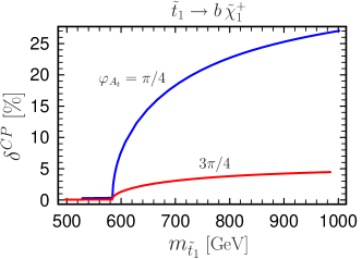
Figure 2: $\delta^{CP}$ as a function of $m_{\tilde{t}_{1}}$ ($M_{\tilde{Q}}$ varied) for various values of $\varphi_{A_{t}}$

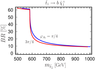
Figure 3: $BR$ as a function of $m_{\tilde{t}_{1}}$ ($M_{\tilde{Q}}$ varied) for various values of $\varphi_{A_{t}}$

This feature can be seen in detail in Fig. 4. If $\tilde{t}_{1}\to\tilde{g}\,t$ is possible, $\delta^{CP}$ is large but $BR$ is small. The other decay channels are $\tilde{t}_{1}\to t\,\widetilde{\chi}^{0}_{i},b\,\widetilde{\chi}^{+}_{2}$.

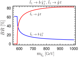
Figure 4: Comparison of $BR(\tilde{t}_{1}\to b\,\widetilde{\chi}^{+}_{1})$ and $BR(\tilde{t}_{1}\to\tilde{g}\,t)$ as a function of $m_{\tilde{t}_{1}}$ ($M_{\tilde{Q}}$ varied)

We also studied the dependence on the gluino phase $\varphi_{\tilde{g}}$ as a second source of CP violation, which is, however, in conflict with the current EDM limit of mercury by a factor of two.

Figure 5 shows the contributions from the self-energy and vertex graphs with gluino exchange (see Fig. 1) as a function of $m_{\tilde{t}_{1}}$. As already anticipated in Section 3, the gluino self-energy loop dominates.

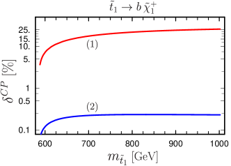
Figure 5: Contribution of the gluino self-energy loop (1) and the vertex correction (2) to $\delta^{CP}$ as a function of $m_{\tilde{t}_{1}}$ ($M_{\tilde{Q}}$ varied)

In Fig. 6 we show the ratios of $\delta^{CP}$ between the approximated formula for the gluino self-energy loop $\delta^{CP}_{\mathrm{approx}}$ (Eq. (18)) and all one-loop contributions $\delta^{CP}_{\mathrm{all}}$, as well as between both gluino contributions $\delta^{CP}_{\tilde{g}}$ and all contributions. Above the threshold of $\tilde{t}_{1}\to\tilde{g}\,t$ both gluino processes account for $\sim\!97\%$ of all processes. One can see that $\delta^{CP}_{\mathrm{approx}}$ is indeed a good approximation of $\delta^{CP}_{\mathrm{all}}$.

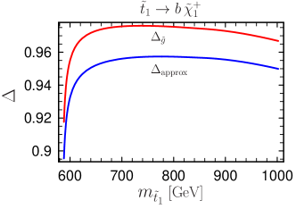
Figure 6: Ratios of $\Delta_{\mathrm{approx}}=\delta^{CP}_{\mathrm{approx}}/\delta^{CP}_{\mathrm{all}}$, see Eq. (18), and $\Delta_{\tilde{g}}=\delta^{CP}_{\tilde{g}}/\delta^{CP}_{\mathrm{all}}$ as a function of $m_{\tilde{t}_{1}}$ ($M_{\tilde{Q}}$ varied)

We also studied the dependence of $\delta^{CP}$ on $\tan\beta$ and $|A_{t}|$. The main effect comes from the off-diagonal element in the stop mass matrix $a_{t}=A_{t}^{*}-\mu/\tan\beta$. For $|A_{t}|\sim 190$ GeV and $\tan\beta\sim 6$ the asymmetry has its maximum up to $25\%$ because $a_{t}$ becomes minimal. In this case one has rather degenerate stop masses which enhance the gluino self-energy contribution due to the propagator $\propto 1/(m^{2}_{\tilde{t}_{2}}-m^{2}_{\tilde{t}_{1}})$. For larger values of $|A_{t}|$ and $\tan\beta$ the asymmetry decreases and begins to be in conflict with the EDM limit of mercury.

The effect on the mass splitting of $\tilde{t}_{1}$ and $\tilde{t}_{2}$ is shown in more detail in Fig. 7 and Fig. 8. We fix $m_{\tilde{t}_{1}}=650$ GeV and vary $m_{\tilde{t}_{2}}$ by changing the parameters $M_{\tilde{Q}},M_{\tilde{U}}$. There are two possibilities, $m_{LL}\lessgtr m_{RR}$. In our scenario $\tilde{\chi}^{+}_{1}$ is gaugino-like which couples dominantly to $\tilde{t}_{L}$. For $m_{LL}<m_{RR}$ we have $\tilde{t}_{1}\sim\tilde{t}_{L}$ and $\tilde{t}_{2}\sim\tilde{t}_{R}$. Hence $BR(\tilde{t}_{1}\to b\,\tilde{\chi}^{+}_{1})$ is large, but $\delta^{CP}$ is small because the coupling of the internal $\tilde{t}_{2}$ to $b\,\tilde{\chi}^{+}_{1}$ is suppressed (see left graph of Figure 1). For $m_{LL}>m_{RR}$ one has the opposite behavior. When $\tilde{\chi}^{+}_{1}$ is higgsino-like the whole situation is reversed. We therefore see that for the cases where $\delta^{CP}$ is large the BR is always small and vice versa, unless the masses of $\tilde{t}_{1}$ and $\tilde{t}_{2}$ are rather degenerate. Note that the masses cannot be arbitrarily degenerate, since otherwise the off-diagonal elements in the stop mass matrix (and thus the complex $A_{t}$ parameter as the main source of CP violation) would need to vanish.
Furthermore, it is crucial that the enhancement of $\delta^{CP}$ due to a small stop mass difference is not a resonance enhancement, i.e. the mass difference $m_{\tilde{t}_{2}}-m_{\tilde{t}_{1}}$ must be sufficiently large compared to the FWHM $\Gamma^{\mathrm{total}}_{\tilde{t}_{2}}/2$ of the resonance. In our scenario this is always the case, since $\Gamma^{\mathrm{total}}_{\tilde{t}_{2}}/2=9$ GeV and $\Delta m_{\tilde{t}}=35$ GeV at the reference point and $\Gamma^{\mathrm{total}}_{\tilde{t}_{2}}/2$ always remains much smaller for various mass differences.

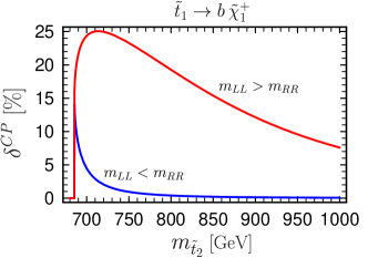
Figure 7: Effect on mass splitting of $\tilde{t}_{1}$ and $\tilde{t}_{2}$ for $\delta^{CP}$ as a function of $m_{\tilde{t}_{2}}$ ($M_{\tilde{Q}},M_{\tilde{U}}$ varied) for $m_{\tilde{t}_{1}}=650$ GeV

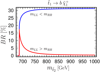
Figure 8: Effect on mass splitting of $\tilde{t}_{1}$ and $\tilde{t}_{2}$ for $BR$ as a function of $m_{\tilde{t}_{2}}$ ($M_{\tilde{Q}},M_{\tilde{U}}$ varied) for $m_{\tilde{t}_{1}}=650$ GeV

For completeness, we also examined the process $\tilde{t}_{2}\to b\,\tilde{\chi}^{+}_{1}$. Because of the similar masses and large mixing of the stops, the resulting plots are alike. We obtain $\delta^{CP}=19\%$ and $BR=17\%$ at the reference point.

We also investigated the influence on the Yukawa couplings $h_{t}$ and $h_{b}$ taken to be running. In our scenario, the difference of the asymmetry $\delta^{CP}$ taken with running and non-running Yukawa couplings is negligible.

The theoretical uncertainty of the asymmetry $\delta^{CP}$ is estimated $\sim\!20\%$, due to higher order corrections Kraml:1996kz ; Guasch:2003ig .

For a measurement of the asymmetry $\delta^{CP}$ (Eq. (1)) at LHC, one has to consider the process

$$pp \to {\tilde{t}}_{1}\bar{\tilde{t}}_{1}+X\to(b\tilde{\chi}_{1}^{+})(\bar{b}\tilde{\chi}_{1}^{-})+X$$ (20)

$$\to (bW^{+}\tilde{\chi}_{1}^{0})(\bar{b}W^{-}\tilde{\chi}_{1}^{0})+X$$

$$\to \textrm{2 b-jets}+W^{+}+W^{-}+\not\!\!E_{T}+X$$

(where $X$ only contains the beam jets) with one $W^{+}$ decaying hadronically and the other one leptonically to get information on the charge of the $W$, and in turn of the chargino and the stop. We assume that the masses of ${\tilde{t}_{1}}$, ${\tilde{t}_{2}}$, $\tilde{\chi}_{1}^{\pm}$ and $\tilde{\chi}_{1}^{0}$ are known so that one has enough kinematical constraints to single out the respective decays MoortgatPick:2010wp . In such a way it should also be possible to separate off the production and decay of ${\tilde{t}_{1}}$ from those of ${\tilde{t}_{2}}$. For $\sqrt{s}=14$ TeV, $m_{\tilde{t}_{1}}=610$ GeV the cross section of $pp\to{\tilde{t}}_{1}\bar{\tilde{t}}_{1}$ is $\sigma=200$ fb at NLO according to Prospino Beenakker1998 . Assuming ${\cal L}=300\,\mathrm{fb}^{-1}$ and $BR(\tilde{t}_{1}\to b\,\tilde{\chi}^{+}_{1})=0.2$ we estimate a purely statistical relative error of the asymmetry $\Delta\delta^{CP}/\delta^{CP}=\pm 0.077$. The largest background is of course pair production of top quarks Dydak1996 . For a realistic estimate of the measurability a Monte Carlo study would be necessary, which is, however, beyond the scope of this article. For the same decay chain of ${\tilde{t}_{1}}$ such a study was done for an $e^{+}e^{-}$ collider Bartl:2009rt .

5 Conclusions

In the MSSM with complex parameters, loop corrections to the $\tilde{t}_{i}\to b\,\widetilde{\chi}^{+}_{k}$ decay can lead to a CP violating decay rate asymmetry $\delta^{CP}$. We studied this asymmetry at full one-loop level, analyzing the dependence on the parameters and phases. Below the threshold of the $\tilde{t}_{i}\to\tilde{g}\,t$ decay, $\delta^{CP}$ is $<\!1\%$. If this channel is open, a $\delta^{CP}$ up to $25\%$ is possible (mainly due to the gluino contribution in the self-energy loop), if the stop particles have a small mass splitting together with large mixing and the chargino is wino like.

Appendix A Masses and Mixing Matrices

The sfermion mass matrix in the basis $(\tilde{f}_{L},\tilde{f}_{R})$ with $\tilde{f}=\tilde{t},\tilde{b},\tilde{\tau},\dots$ is

$${\cal M}_{\tilde{f}}^{2}=\left(\begin{array}[]{cc}m_{\tilde{f}_{L}}^{2}&m_{f}a_{f}\\ m_{f}a_{f}^{*}&m_{\tilde{f}_{R}}^{2}\end{array}\right)$$ (21)

with the following entries

$$m_{\tilde{f}_{L}}^{2} = M_{\{\tilde{Q};\tilde{L}\}}^{2}+m_{f}^{2}$$ (22)

$$+m_{Z}^{2}\cos 2\beta(I_{f}^{3L}-e_{f}\sin^{2}\theta_{W})\,,$$

$$m_{\tilde{f}_{R}}^{2} = M_{\{\tilde{U};\tilde{D};\tilde{E}\}}^{2}+m_{f}^{2}+m_{Z}^{2}\cos 2\beta\,e_{f}\sin^{2}\theta_{W}\,,$$ (23)

$$m_{f}a_{f} = \biggl{\{}\begin{array}[]{l}m_{u}(A_{u}^{*}-\mu\cot\beta)\;\dots\;\textnormal{up-type sfermion}\,,\\ m_{d}(A_{d}^{*}-\mu\tan\beta)\;\dots\;\textnormal{down-type sfermion}\,.\end{array}$$ (25)

For the stops ($\tilde{f}=\tilde{t}$) we simply insert the corresponding values $I_{t}^{3L}=1/2$, $e_{t}=2/3$, $M_{\tilde{Q}}$, $M_{\tilde{U}}$, $m_{t}$ and $A_{t}$. Analogously, for the sbottoms ($\tilde{f}=\tilde{b}$) we have $I_{b}^{3L}=-1/2$, $e_{b}=-1/3$, $M_{\tilde{Q}}$, $M_{\tilde{D}}$, $m_{b}$ and $A_{b}$.
${\cal M}_{\tilde{f}}^{2}$ is diagonalized by the rotation matrix $R^{\tilde{f}}$ such that $R^{\tilde{f}}{\cal M}_{\tilde{f}}^{2}\,(R^{\tilde{f}})^{\dagger}={\rm diag}(m_{\tilde{f}_{1}}^{2},m_{\tilde{f}_{2}}^{2})$ and ${\tilde{f}_{1}\choose\tilde{f}_{2}}=R^{\tilde{f}}{\tilde{f}_{L}\choose\tilde{f}_{R}}$. We have

$$R^{\tilde{f}}=\left(\begin{array}[]{cc}R^{\tilde{f}}_{1L}&R^{\tilde{f}}_{1R}\\ R^{\tilde{f}}_{2L}&R^{\tilde{f}}_{2R}\end{array}\right)=\left(\begin{array}[]{cc}\cos\theta_{\tilde{f}}&e^{i\varphi_{\tilde{f}}}\sin\theta_{\tilde{f}}\\ -e^{-i\varphi_{\tilde{f}}}\sin\theta_{\tilde{f}}&\cos\theta_{\tilde{f}}\end{array}\right).$$ (27)

Using the unitarity property of the sfermion rotation matrices and the diagonalization equation for the sfermion mass matrix,

$${\cal M}_{\tilde{f}}^{2}=\left(\begin{array}[]{cc}m_{\tilde{f}_{L}}^{2}&m_{f}a_{f}\\ m_{f}a_{f}^{*}&m_{\tilde{f}_{R}}^{2}\end{array}\right)=(R^{\tilde{f}})^{\dagger}\left(\begin{array}[]{cc}m_{\tilde{f}_{1}}^{2}&0\\ 0&m_{\tilde{f}_{2}}^{2}\end{array}\right)R^{\tilde{f}}\,,$$ (28)

one can derive the following relations (we define $\Delta^{\tilde{f}}=1/(m_{\tilde{f}_{2}}^{2}-m_{\tilde{f}_{1}}^{2})$):

$$R^{\tilde{f}}_{22}R^{\tilde{f}*}_{21} = -R^{\tilde{f}}_{12}R^{\tilde{f}*}_{11}=m_{f}a_{f}\Delta^{\tilde{f}}\,,$$

$$R^{\tilde{f}}_{21}R^{\tilde{f}*}_{22} = -R^{\tilde{f}}_{11}R^{\tilde{f}*}_{12}=m_{f}a_{f}^{*}\Delta^{\tilde{f}}\,,$$

$$R^{\tilde{f}}_{11}R^{\tilde{f}*}_{11} = R^{\tilde{f}}_{22}R^{\tilde{f}*}_{22}=(m_{\tilde{f}_{2}}^{2}-m_{\tilde{f}_{L}}^{2})\Delta^{\tilde{f}}\,,$$

$$R^{\tilde{f}}_{12}R^{\tilde{f}*}_{12} = R^{\tilde{f}}_{21}R^{\tilde{f}*}_{21}=-(m_{\tilde{f}_{1}}^{2}-m_{\tilde{f}_{L}}^{2})\Delta^{\tilde{f}}\,.$$ (29)

The chargino mass matrix in the basis $(-i\lambda^{+},\psi^{1}_{H_{2}})$ is

$${\cal M}_{C}=\left(\begin{array}[]{cc}M_{2}&\sqrt{2}\,m_{W}\sin\beta\\ \sqrt{2}\,m_{W}\cos\beta&\mu\end{array}\right).$$ (30)

It is diagonalized by the two unitary matrices $U$ and $V$

$$U^{*}{\cal M}_{C}V^{\dagger}={\rm diag}(m_{\tilde{\chi}^{\pm}_{1}},m_{\tilde{\chi}^{\pm}_{2}})\,,$$ (31)

where $m_{\tilde{\chi}^{\pm}_{1,2}}$ are the masses of the physical chargino states.

Appendix B Interaction Lagrangian

In this section we give the parts of the interaction Lagrangian that we need for the calculation of the leading contributions. The chargino-squark-quark interaction is described by

$${\cal L}_{\tilde{\chi}^{+}q\tilde{q}^{\prime}} = \bar{t}(A^{R}_{ki}P_{R}+A^{L}_{ki}P_{L})\tilde{\chi}^{+}_{k}\,\tilde{b}_{i}$$ (32)

$$+\bar{b}(B^{R}_{ki}P_{R}+B^{L}_{ki}P_{L})\tilde{\chi}^{+c}_{k}\,\tilde{t}_{i}$$

$$+\overline{\tilde{\chi}^{+}_{k}}(A^{L*}_{ki}P_{R}+A^{R*}_{ki}P_{L})t\,\tilde{b}^{*}_{i}$$

$$+\overline{\tilde{\chi}^{+c}_{k}}(B^{L*}_{ki}P_{R}+B^{R*}_{ki}P_{L})b\,\tilde{t}^{*}_{i}\,.$$

The couplings are

$$A^{R}_{ki} = h^{*}_{b}R^{\tilde{b}*}_{i2}U_{k2}-gR^{\tilde{b}*}_{i1}U_{k1}$$

$$= \frac{g}{\sqrt{2}}\left(\frac{m_{b}}{m_{W}\cos\beta}U_{k2}R^{\tilde{b}*}_{i2}-\sqrt{2}U_{k1}R^{\tilde{b}*}_{i1}\right)\,,$$

$$A^{L}_{ki} = h_{t}R^{\tilde{b}*}_{i1}V^{*}_{k2}=\frac{gm_{t}}{\sqrt{2}m_{W}\sin\beta}V^{*}_{k2}R^{\tilde{b}*}_{i1}\,,$$

$$B^{R}_{ki} = h^{*}_{t}R^{\tilde{t}*}_{i2}V_{k2}-gR^{\tilde{t}*}_{i1}V_{k1}$$

$$= \frac{g}{\sqrt{2}}\left(\frac{m_{t}}{m_{W}\sin\beta}V_{k2}R^{\tilde{t}*}_{i2}-\sqrt{2}V_{k1}R^{\tilde{t}*}_{i1}\right)\,,$$

$$B^{L}_{ki} = h_{b}R^{\tilde{t}*}_{i1}U^{*}_{k2}=\frac{gm_{b}}{\sqrt{2}m_{W}\cos\beta}U^{*}_{k2}R^{\tilde{t}*}_{i1}\,,$$ (33)

where we used the relations $m_{t}=(h_{t}\,\nu\sin\beta)/\sqrt{2}$, $m_{b}=(h_{b}\,\nu\cos\beta)/\sqrt{2}$ and $m_{W}=g\nu/2$ to convert the coefficients.
The gluino-squark-quark interaction is

$${\cal L}_{\tilde{g}q\tilde{q}} = \overline{\tilde{g}_{\alpha}}(G^{R\alpha}_{i;uv}P_{R}+G^{L\alpha}_{i;uv}P_{L})q^{u}\tilde{q}^{\,v*}_{i}$$ (34)

$$+\overline{q^{u}}(G^{L\alpha*}_{i;uv}P_{R}+G^{R\alpha*}_{i;uv}P_{L})\tilde{g}_{\alpha}\,\tilde{q}^{\,v}_{i}\,,$$

where we used $u,v$ as the color index ($u,v=1,2,3$), $i$ as the mass index ($i=1,2$) and $\alpha$ as the gluon/gluino index ($\alpha=1,\ldots,8$). The couplings are

$$G^{R\alpha}_{i;uv} = T^{\alpha}_{uv}G^{R}_{i}\quad{\rm with}\ G^{R}_{i}=\sqrt{2}\,g_{s}R^{\tilde{q}}_{i2}\,e^{i\frac{\varphi_{\tilde{g}}}{2}}\,,$$

$$G^{L\alpha}_{i;uv} = T^{\alpha}_{uv}G^{L}_{i}\quad{\rm with}\ G^{L}_{i}=-\sqrt{2}\,g_{s}R^{\tilde{q}}_{i1}\,e^{-i\frac{\varphi_{\tilde{g}}}{2}}$$ (35)

with $T^{\alpha}_{uv}$ as the generator of the $\mathrm{SU(3)_{C}}$ group, $g_{s}$ as the coupling constant of the strong interaction and $\varphi_{\tilde{g}}$ as the gluino mass phase.

References

• (1) M. Dugan, B. Grinstein, and L. J. Hall, Nucl. Phys. B255, 413 (1985).
• (2) T. Ibrahim and P. Nath, Phys. Rev. D57, 478 (1998), arXiv:hep-ph/9708456.
• (3) M. Brhlik, G. J. Good, and G. L. Kane, Phys. Rev. D59, 115004 (1999), arXiv:hep-ph/9810457.
• (4) A. Bartl, T. Gajdosik, W. Porod, P. Stockinger, and H. Stremnitzer, Phys. Rev. D60, 073003 (1999), arXiv:hep-ph/9903402.
• (5) A. Pilaftsis, Nucl. Phys. B644, 263 (2002), arXiv:hep-ph/0207277.
• (6) A. Bartl, W. Majerotto, W. Porod, and D. Wyler, Phys. Rev. D68, 053005 (2003), arXiv:hep-ph/0306050.
• (7) V. D. Barger et al., Phys. Rev. D64, 056007 (2001), arXiv:hep-ph/0101106.
• (8) M. Pospelov and A. Ritz, Annals Phys. 318, 119 (2005), arXiv:hep-ph/0504231.
• (9) K. A. Olive, M. Pospelov, A. Ritz, and Y. Santoso, Phys. Rev. D72, 075001 (2005), arXiv:hep-ph/0506106.
• (10) S. Abel and O. Lebedev, JHEP 01, 133 (2006), arXiv:hep-ph/0508135.
• (11) S. Yaser Ayazi and Y. Farzan, Phys. Rev. D74, 055008 (2006), arXiv:hep-ph/0605272.
• (12) J. R. Ellis, J. S. Lee, and A. Pilaftsis, JHEP 10, 049 (2008), arXiv:0808.1819.
• (13) T. Gajdosik, Acta Physica Polonica B40, 3171 (2009), arXiv:0910.3512.
• (14) S. Kraml, Proceedings of SUSY07, Karlsruhe, Germany, 26 Jul - 1 Aug 2007 , 132 (2007), arXiv:0710.5117.
• (15) E. Christova, H. Eberl, W. Majerotto, and S. Kraml, Nucl. Phys. B639, 263 (2002), arXiv:hep-ph/0205227.
• (16) E. Christova, H. Eberl, E. Ginina, and W. Majerotto, JHEP 02, 075 (2007), arXiv:hep-ph/0612088.
• (17) E. Christova, H. Eberl, W. Majerotto, and S. Kraml, JHEP 12, 021 (2002), arXiv:hep-ph/0211063.
• (18) E. Christova, E. Ginina, and M. Stoilov, JHEP 11, 027 (2003), arXiv:hep-ph/0307319.
• (19) E. Ginina, contributed to 4th Advanced Research Workshop: Gravity, Astrophysics, and Strings at the Black Sea, Kiten, Bourgas, Bulgaria, 10-16 Jun 2007 (2008), arXiv:0801.2344.
• (20) E. Christova, H. Eberl, and E. Ginina, Talk given at Prospects for Charged Higgs Discovery at Colliders (CHARGED 2008), Uppsala, Sweden, 16-19 Sep 2008 (2008), arXiv:0812.0265.
• (21) E. Christova, H. Eberl, E. Ginina, and W. Majerotto, Phys. Rev. D79, 096005 (2009), arXiv:0812.4392.
• (22) M. Frank and I. Turan, Phys. Rev. D76, 076008 (2007), arXiv:0708.0026.
• (23) M. Frank and I. Turan, Phys. Rev. D76, 016001 (2007), arXiv:hep-ph/0703184.
• (24) A. Arhrib, R. Benbrik, M. Chabab, W. T. Chang, and T.-C. Yuan, Int. J. Mod. Phys. A22, 6022 (2008), arXiv:0708.1301.
• (25) H. Eberl, T. Gajdosik, W. Majerotto, and B. Schrausser, Phys. Lett. B618, 171 (2005), arXiv:hep-ph/0502112.
• (26) J. Ellis, F. Moortgat, G. Moortgat-Pick, J. M. Smillie, and J. Tattersall, Eur. Phys. J. C60, 633 (2009), arXiv:0809.1607.
• (27) F. Deppisch and O. Kittel, JHEP 09, 110 (2009), arXiv:0905.3088.
• (28) G. Moortgat-Pick, K. Rolbiecki, J. Tattersall, and P. Wienemann, JHEP 01, 004 (2010), arXiv:0908.2631.
• (29) S. M. R. Frank and H. Eberl, AIP Conf. Proc. 1200, 518 (2010), arXiv:0910.0154.
• (30) S. Frank, CP Violating Asymmetries Induced by Supersymmetry, Master’s thesis, Johannes Kepler University Linz, 2008, arXiv:0909.3969.
• (31) G. Passarino and M. J. G. Veltman, Nucl. Phys. B160, 151 (1979).
• (32) A. Denner, Fortschr. Phys. 41, 307 (1993), arXiv:0709.1075.
• (33) T. Hahn, Comput. Phys. Commun. 140, 418 (2001), arXiv:hep-ph/0012260.
• (34) J. S. Lee, M. Carena, J. Ellis, A. Pilaftsis, and C. E. M. Wagner, Comput. Phys. Commun. 180, 312 (2009), arXiv:0712.2360.
• (35) Particle Data Group, C. Amsler et al., Phys. Lett. B667, 1 (2008), and 2009 partial update for the 2010 edition.
• (36) W. C. Griffith et al., Phys. Rev. Lett. 102, 101601 (2009).
• (37) WMAP, E. Komatsu et al., Astrophys. J. Suppl. 180, 330 (2009), arXiv:0803.0547.
• (38) G. Belanger, F. Boudjema, S. Kraml, A. Pukhov, and A. Semenov, Phys. Rev. D73, 115007 (2006), arXiv:hep-ph/0604150.
• (39) G. Belanger, F. Boudjema, A. Pukhov, and A. Semenov, Comput. Phys. Commun. 176, 367 (2007), arXiv:hep-ph/0607059.
• (40) Heavy Flavor Averaging Group, E. Barberio et al., (2008), arXiv:0808.1297, and online update at http://www.slac.stanford.edu/xorg/hfag.
• (41) S. Kraml, H. Eberl, A. Bartl, W. Majerotto, and W. Porod, Phys. Lett. B386, 175 (1996), arXiv:hep-ph/9605412.
• (42) J. Guasch, W. Hollik, and J. Sola, (2003), arXiv:hep-ph/0307011.
• (43) G. Moortgat-Pick, K. Rolbiecki, and J. Tattersall, (2010), arXiv:1008.2206.
• (44) W. Beenakker, M. Kramer, T. Plehn, M. Spira, and P. M. Zerwas, Nucl. Phys. B515, 3 (1998), arXiv:hep-ph/9710451.
• (45) U. Dydak, CMS TN/96-022 (1996).
• (46) A. Bartl, W. Majerotto, K. Monig, A. N. Skachkova, and N. B. Skachkov, Phys. Part. Nucl. Lett. 6, 181 (2009), arXiv:0906.3805.