Finding the Maximizers of the Information Divergence from an Exponential Family

Abstract

This paper investigates maximizers of the information divergence from an exponential family $\mathcal{E}$. It is shown that the $rI$-projection of a maximizer $P$ to $\mathcal{E}$ is a convex combination of $P$ and a probability measure $P_{-}$ with disjoint support and the same value of the sufficient statistics $A$. This observation can be used to transform the original problem of maximizing $D(\cdot||\mathcal{E})$ over the set of all probability measures into the maximization of a function $\overline{D}_{r}$ over a convex subset of $\ker A$. The global maximizers of both problems correspond to each other. Furthermore, finding all local maximizers of $\overline{D}_{r}$ yields all local maximizers of $D(\cdot||\mathcal{E})$.

This paper also proposes two algorithms to find the maximizers of $\overline{D}_{r}$ and applies them to two examples, where the maximizers of $D(\cdot||\mathcal{E})$ were not known before.

1 Introduction

Let $\mathcal{X}$ be a finite set of cardinality $N$ and consider an exponential family $\mathcal{E}$ on $\mathcal{X}$. In this work this will mean that there exists a real-valued $h\times N$ matrix $A$ (whose columns $A_{x}$ are indexed by $x\in\mathcal{X}$) and a reference measure $r$ on $\mathcal{X}$ satisfying $r(x)>0$ for all $x\in\mathcal{X}$ such that $\mathcal{E}$ consists of all probability measures on $\mathcal{X}$ of the form

$$P_{\theta}(x)=\frac{r(x)}{Z_{\theta}}\exp\left(\sum_{i=1}^{h}\theta_{i}A_{i,x}\right).$$ (1)

In this formula $\theta\in\mathbb{R}^{h}$ is a vector of parameters and $Z_{\theta}$ ensures normalization. The matrix $A$ is called the sufficient statistics of $\mathcal{E}$. For technical reasons it will be assumed that the row span of $A$ contains the constant vector $(1,\dots,1)$, see section 2. The topological closure of $\mathcal{E}$ will be denoted by $\overline{\mathcal{E}}$.

The information divergence (also known as the Kullback-Leibler divergence or relative entropy) of two probability distributions $P$, $Q$ is defined as

$$D(P||Q)=\sum_{x\in\mathcal{X}}P(x)\log\left(\frac{P(x)}{Q(x)}\right).$$ (2)

Here we define $0\log 0=0\log(0/0)=0$. It is strictly positive unless $P=Q$, and it is infinite if the support of $P$ is not contained in the support of $Q$.

With these definitions Nihat Ay proposed the following problem, motivated by probabilistic models for evolution and learning in neural networks based on the infomax principle [2]:

• Given an exponential family $\mathcal{E}$, which probability measures $P$ maximize $D(P||\mathcal{E})$?

Here $D(P||\mathcal{E})=\inf_{Q\in\mathcal{E}}D(P||Q)$.

Already [2] contains a lot of properties of the maximizers, like the projection property and support restrictions, but only in the case where the $rI$-projection $P_{\mathcal{E}}$ of the maximizer lies in $\mathcal{E}$. The projection property means that the maximizer $P$ satisfies $P(x)=P_{\mathcal{E}}(\mathcal{Z})P_{\mathcal{E}}(x)$ for all $x\in\mathcal{Z}:=\operatorname{supp}(P)$. In [13] František Matúš computed the first order optimality conditions in the general case, showing that the projection property also holds if $P_{\mathcal{E}}\in\overline{\mathcal{E}}\setminus\mathcal{E}$. For further results on the maximization problem see [3, 14, 15].

In this work it is shown that the original maximization problem can be solved by studying the related problem:

• Maximize the function $\overline{D}_{r}(u)=\sum_{x\in X}u(x)\log\frac{|u(x)|}{r(x)}$ for all $u\in\ker A$ such that $||u||_{1}\leq 2$ and $\sum_{x}u_{x}=0$.

Here, $||u||_{1}$ is the $\ell_{1}$-norm of $u$. Theorem 3 will show that there is a bijection between the global maximizers of these two maximization problems. Furthermore, knowing all local maximizers of $\overline{D}_{r}$ yields all local maximizers of $D(\cdot||\mathcal{E})$. This relation is a consequence of the projection property mentioned above.

In Section 2 some known properties of exponential families and the information divergence are collected, including Matúš’s result on the first order optimality conditions of maximizers of $D(\cdot||\mathcal{E})$. In Section 3 the projection property is analyzed. It is easy to see that probability measures that satisfy the projection property and that do not belong to $\mathcal{E}$ come in pairs $(P_{+},P_{-})$ such that $P_{+}-P_{-}\in\ker A\setminus\{0\}$. This pairing is used in Section 4 to replace the original problem by the maximization of the function $\overline{D}_{r}$. Theorem 3 in this section investigates the relation between the maximizers of both problems. In Section 5 the first order conditions of $\overline{D}_{r}$ are computed. Section 6 discusses the case where $\dim\ker A=1$, demonstrating how the reformulation leads to a quick solution of the original problem. Section 7 gives some ideas how to solve the critical equations from Section 5. Section 8 presents an alternative method of computing the local maximizers of $D(\cdot||\mathcal{E})$, which uses the projection property more directly. Sections 7 and 8 contain two examples which demonstrate how the theory of this paper can be put to practical use.

2 Exponential families and the information divergence

The definition of an exponential family, as it will be used in this work, was already stated in the introduction. It is important to note that the correspondence between exponential families $\mathcal{E}$ on one side and sufficient statistics $A$ and reference measure $r$ on the other side is not unique. One reason for this lies in the normalization of probability measures: We can always add a constant row to the matrix $A$ without changing $\mathcal{E}$ (as a set). For this reason in the following it will be assumed that $A$ contains the constant row $(1,\dots,1)$ in its row space. This implies that every $u\in\ker A$ satisfies $\sum_{x\in\mathcal{X}}u(x)=0$.

In order to characterize the remaining ambiguity in the parametrization $(r,A)\mapsto\mathcal{E}$, denote by $\mathcal{E}_{r,A}$ the exponential family associated to a given matrix $A$ and a given reference measure. Then $\mathcal{E}_{r,A}=\mathcal{E}_{r^{\prime},A^{\prime}}$ as sets if and only if the following two conditions are satisfied:

• $r\in\mathcal{E}_{r^{\prime},A^{\prime}}$.

• The row span of $A$ equals the row span of $A^{\prime}$.

The introduction also featured the definition of the information divergence. In the following we will also use formula (2) for positive measures $Q$ which are not necessarily normalized. In this case

$$D(P||\lambda Q)=\sum_{x}P(x)\log\frac{P(x)}{\lambda Q(x)}=D(P||Q)-\log\lambda\quad\text{ for all }\lambda>0,$$ (3)

where $\sum_{x}P(x)=1$ was used.

The following theorem sums up the main facts about exponential families:

Theorem A.

Let $P$ be a probability measure on $\mathcal{X}$. Then there exists a unique probability measure $P_{\mathcal{E}}$ in $\overline{\mathcal{E}}$ such that $AP=AP_{\mathcal{E}}$. Furthermore, $P_{\mathcal{E}}$ has the following properties:

1. For all $Q\in\mathcal{E}$

   $$D(P||Q)=D(P||P_{\mathcal{E}})+D(P_{\mathcal{E}}||Q).$$ (4)

2. $P_{\mathcal{E}}$ satisfies

   $$D(P||\mathcal{E})=H_{r}(P_{\mathcal{E}})-H_{r}(P)$$ (5)

3. $P_{\mathcal{E}}$ maximizes the concave function

   $$H_{r}(Q):=-\sum_{x}Q(x)\log\frac{Q(x)}{r(x)}$$ (6)

   subject to the condition $AQ=AP$.

Sketch of proof.

Corollary 3.1 of [7] proves existence and uniqueness of $P_{\mathcal{E}}$ and the “Pythagorean identity” (4) for all probability measures $P$ and all probability measures $Q\in\overline{\mathcal{E}}$. It follows from (3) that

$$D(P||r)=D(P||P_{\mathcal{E}})+D(P_{\mathcal{E}}||r),$$ (7)

so statements 2. and 3. follow from $H_{r}(Q)=-D(Q||r)$. ∎

$P_{\mathcal{E}}$ is called the $rI$-projection of $P$ to $\mathcal{E}$, or simply the projection of $P$ to $\mathcal{E}$.

Note that the function $H_{r}$ introduced in the theorem satisfies $H_{r}(P)=-D(P||r)$. It can thus be interpreted as a negative relative entropy. In this work $H_{r}$ is prefered to its negative counterpart in order to keep the connection to the entropy $H$ visible in the important case that $r(x)=1$ for all $x\in\mathcal{X}$.

The map associated to the matrix $A$ is called the moment map. It maps the set of all probability measures on $\mathcal{X}$ onto the polytope $\mathcal{M}$ which is the convex hull of the columns of $A$. This polytope is called the convex support of $\mathcal{E}$. In the special case that $\mathcal{E}$ is a hierarchical model (see [12]), $\mathcal{M}$ is called the marginal polytope of $\mathcal{E}$.

Note that we can associate a point $A_{x}\in\mathcal{M}$ with each state $x\in\mathcal{X}$. Among these points are the vertices of $\mathcal{M}$, but not every point $A_{x}$ needs to be a vertex of $\mathcal{M}$.

Theorem B.

Let $P_{+}$ be a (local) maximizer of $D(\cdot||\mathcal{E})$ with support $\mathcal{Z}=\operatorname{supp}(P_{+})$ and $P_{\mathcal{E}}$ its $rI$-projection to $\mathcal{E}$. Then the following holds:

1. $P_{+}$ satisfies the projection property, i.e., up to normalization $P_{+}$ equals the restriction of $P_{\mathcal{E}}$ to $\mathcal{Z}$:

   $$P_{+}(x)=\begin{cases}\frac{P_{\mathcal{E}}(x)}{P_{\mathcal{E}}(\mathcal{Z})},&\text{ if }x\in\mathcal{Z},\\ 0,&\text{ else.}\end{cases}$$ (8)

2. Suppose $\mathcal{Y}:=\operatorname{supp}(P_{\mathcal{E}})\neq\mathcal{X}$. Then the moment map maps $\mathcal{Y}$ and $\mathcal{X}\setminus\mathcal{Y}$ into parallel hyperplanes.

3. The cardinality of $\mathcal{Z}$ is bounded by $\dim\mathcal{E}+1$.

Proof.

Statements 1. and 3. were already known to Ay[2] in the special case where $\mathcal{Y}=\mathcal{X}$. The general form of statement 3. is Proposition 3.2 of [15]. Statement 2. and the generalization of statement 1. are due to Matúš[13, Theorem 5.1]. ∎

The paper [13] contains further conditions on the maximizer. However, these will not be studied in this work.

Definition 1.

Any probability measure $P$ that satisfies (8) will be called a projection point. If $P$ satisfies conditions 1. and 2. of Theorem B, then $P$ will be called a quasi-critical point of $D(\cdot||\mathcal{E})$, or a $D$-quasi-critical point.

3 Projection points

In this section assume that $A$ does not have full rank. Otherwise the function $D(\cdot||\mathcal{E})$ is trivial.

Let $P_{+}$ be a projection point, and let $P_{\mathcal{E}}$ be its projection to $\mathcal{E}$. Denote $\mathcal{Z}=\operatorname{supp}(P_{+})$ and $\mathcal{Y}=\operatorname{supp}(P_{\mathcal{E}})$. Every measure $P_{\lambda}:=\lambda P_{+}+(1-\lambda)P_{\mathcal{E}}$ on the line through $P_{+}$ and $P_{\mathcal{E}}$ is normalized and has the same sufficient statistics as $P_{+}$ and $P_{\mathcal{E}}$. Fix $\lambda_{-}=-\frac{P_{\mathcal{E}}(\mathcal{Z})}{1-P_{\mathcal{E}}(\mathcal{Z})}$. Then

$$P_{\lambda_{-}}(x)=\begin{cases}-\frac{P_{\mathcal{E}}(\mathcal{Z})}{1-P_{\mathcal{E}}(\mathcal{Z})}\frac{P_{\mathcal{E}}(x)}{P_{\mathcal{E}}(\mathcal{Z})}+\frac{1}{1-P_{\mathcal{E}}(\mathcal{Z})}P_{\mathcal{E}}(x)=0&\text{ if }x\in\mathcal{Z},\\ (1-\lambda_{-})P_{\mathcal{E}}(x)=\frac{1+P_{\mathcal{E}}(\mathcal{Z})}{1-P_{\mathcal{E}}(\mathcal{Z})}P_{\mathcal{E}}(x)\geq 0&\text{ else.}\end{cases}$$ (9)

Thus $P_{-}:=P_{\lambda_{-}}$ is a probability measure with support equal to $\mathcal{Y}\setminus\mathcal{Z}$, and $u:=P_{+}-P_{-}$ lies in the kernel of $A$. Furthermore, $P_{-}$ is a second projection point with the same projection $P_{\mathcal{E}}$ to $\mathcal{E}$ as $P_{+}$.

The projection $P_{\mathcal{E}}$ can be written as a convex combination of $P_{+}$ and $P_{-}$, i.e., $P_{\mathcal{E}}=\mu P_{+}+(1-\mu)P_{-}$, where $\mu=\frac{\lambda_{-}}{\lambda_{-}-1}\in(0,1)$. Since the supports of $P_{+}$ and $P_{-}$ are disjoint we have $\mu=P_{\mathcal{E}}(\mathcal{Z})$ and $(1-\mu)=P_{\mathcal{E}}(\mathcal{X}\setminus\mathcal{Z})$. In other words,

$$P_{\mathcal{E}}(x)=\begin{cases}\mu P_{+}(x),&x\in\mathcal{Z},\\ (1-\mu)P_{-}(x),&x\notin\mathcal{Z}.\end{cases}$$ (10)

There are a lot of relations between $P_{+}$, $P_{-}$ and $P_{\mathcal{E}}$. They will be collected in the following Lemma in a slightly more general form.

Lemma 2.

Let $P_{+}$ and $P_{-}$ be two probability measures with disjoint supports such that $AP_{+}=AP_{-}$. Let $\hat{P}$ be the unique probability measure in the convex hull of $P_{+}$ and $P_{-}$ that maximizes the function

$$H_{r}(Q)=-\sum_{x}Q(x)\log\frac{Q(x)}{r(x)}.$$ (11)

Define $\mu=\hat{P}(\mathcal{Z})$, where $\mathcal{Z}=\operatorname{supp}(P_{+})$. Then the following equations hold:

$$\exp(H_{r}(\hat{P}))=\exp(H_{r}(P_{+}))+\exp(H_{r}(P_{-})),$$ (12a)

$$\frac{\mu}{1-\mu}=\exp\left(H_{r}(P_{+})-H_{r}(P_{-})\right),$$ (12b)

$$D(P_{+}||\hat{P})=H_{r}(P_{\mathcal{E}})-H_{r}(P_{+})=\log(1+\exp(H_{r}(P_{-})-H_{r}(P_{+}))).$$ (12c)

Proof.

The first observation is

$$H_{r}(P_{\mathcal{E}})=\mu H_{r}(P_{+})+(1-\mu)H_{r}(P_{-})+h(\mu,1-\mu),$$ (13)

where $h(\mu,1-\mu)=-\mu\log(\mu)-(1-\mu)\log(1-\mu)$.

Since $P_{\mathcal{E}}$ maximizies $H_{r}$ among all probability measures with the same sufficient statistics as $P_{+}$ and $P_{-}$, it follows that

$$\left.\frac{\partial\left(\mu^{\prime}H_{r}(P_{+})+(1-\mu^{\prime})H_{r}(P_{-})+h(\mu^{\prime},1-\mu^{\prime})\right)}{\partial\mu^{\prime}}\right|_{\mu^{\prime}=\mu}=\\ =H_{r}(P_{+})-H_{r}(P_{-})+\log(1-\mu)-\log(\mu)$$

must vanish, which rewrites to

$$\frac{\mu}{1-\mu}=\exp\left(H_{r}(P_{+})-H_{r}(P_{-})\right),$$ (14)

or

$$\mu=\frac{\exp(H_{r}(P_{+}))}{\exp(H_{r}(P_{+}))+\exp(H_{r}(P_{-}))}=\frac{1}{1+\exp(H_{r}(P_{-})-H_{r}(P_{+}))}.$$ (15)

This implies

$$h(\mu,1-\mu) =-\mu H_{r}(P_{+})+\mu\log\left(\exp(H_{r}(P_{+}))+\exp(H_{r}(P_{-}))\right)$$

$$\qquad-(1-\mu)H_{r}(P_{-})+(1-\mu)\log\left(\exp(H_{r}(P_{+}))+\exp(H_{r}(P_{-}))\right)$$

$$=-\mu H_{r}(P_{+})-(1-\mu)H_{r}(P_{-})+\log\left(\exp(H_{r}(P_{+}))+\exp(H_{r}(P_{-}))\right).$$

Comparison with equation (13) yields

$$\exp(H_{r}(P_{\mathcal{E}}))=\exp(H_{r}(P_{+}))+\exp(H_{r}(P_{-})),$$ (16)

which in turn simplifies (15) to

$$\mu=\exp(H_{r}(P_{+})-H_{r}(P_{\mathcal{E}})).$$ (17)

The Kullback-Leibler divergence equals

$$D(P_{+}||P_{\mathcal{E}})=\sum_{x\in\mathcal{Z}}P_{+}(x)\log\frac{1}{P_{\mathcal{E}}(\mathcal{Z})} =-\log(\mu)$$ (18a)

$$=H_{r}(P_{\mathcal{E}})-H_{r}(P_{+})$$ (18b)

$$=\log(1+\exp(H_{r}(P_{-})-H_{r}(P_{+}))).$$ (18c)

∎

As an easy consequence

$$\exp(-D(P_{+}||\mathcal{E}))+\exp(-D(P_{-}||\mathcal{E}))=1,$$ (19)

from which we see that in general $P_{+}$ and $P_{-}$ will not be both maximizers of $D(\cdot||\mathcal{E})$. Furthermore it follows that $D(P||\mathcal{E})\geq\log(2)$ for any global maximizer $P$ (assuming that $A$ does not have full rank).

4 Decomposition of Kernel Elements

Now suppose that $u$ is an arbitrary nonzero element from the kernel of $A$. Then $u=u_{+}-u_{-}$, where $u_{+}$ and $u_{-}$ are positive vectors of disjoint support. Since $A$ contains the constant vector $(1,\dots,1)$ in its rowspan, it follows that the $\ell_{1}$-norms of $u_{+}$ and $u_{-}$ are equal. Thus $u=d_{u}(P_{+}-P_{-})$, where $d_{u}=||u_{+}||_{1}=||u_{-}||_{1}=\frac{1}{2}||u||_{1}>0$ is called the degree of $u$ and $P_{+}$ and $P_{-}$ are two probability measures with disjoint supports. Since $P_{+}$ and $P_{-}$ have the same image under $A$, they have the same projection to $\mathcal{E}$, which will be denoted by $P_{\mathcal{E}}$.

Let $\hat{P}$ be the convex combination of $P_{+}$ and $P_{-}$ that maximizes $H_{r}$. Note that in general $\hat{P}\neq P_{\mathcal{E}}$. Still Lemma 2 applies. Furthermore

$$D(P_{+}||\mathcal{E})=H_{r}(P_{\mathcal{E}})-H_{r}(P_{+})\geq D(P_{+}||\hat{P})=H_{r}(\hat{P})-H_{r}(P_{+}),$$ (20)

since $P_{\mathcal{E}}$ maximizes $H_{r}$ when the image under $A$ is constrained (see Theorem A).

These facts can be used to relate two different optimization problems. The first one is the maximization of the information divergence from $\mathcal{E}$. The second one is the maximization of the function

$$\overline{D}_{r}:\ker A\to\mathbb{R},u\mapsto\sum_{x}u(x)\log\frac{|u(x)|}{r(x)}$$ (21)

subject to the constraint $d_{u}=\frac{1}{2}||u||_{1}=1$. From what has been said above, if $d_{u}=1$ then $u=Q_{+}-Q_{-}$ for two probability measures $Q_{+},Q_{-}$ with disjoint support, and in this case

$$\overline{D}_{r}(u)=H_{r}(Q_{-})-H_{r}(Q_{-}).$$ (22)

Since $\overline{D}_{r}$ is a continuous function from the compact $\ell_{1}$-sphere of radius $2$ in $\ker A$, a maximum is guaranteed to exist.

Theorem 3.

Let $\mathcal{E}$ be an exponential family with sufficient statistics $A$.

1. If $u=Q_{+}-Q_{-}\in\ker A\setminus\{0\}$ is a global maximizer of $\overline{D}_{r}$ subject to $d_{u}=\frac{1}{2}||u||_{1}=1$, then the positive part $Q_{+}$ of $u$ globally maximizes $D(\cdot||\mathcal{E})$.

2. Let $P_{+}$ be a local maximizer of the information divergence. There exists a unique probability measure $P_{-}$ with support disjoint from $P_{+}$ such that $P_{+}-P_{-}\in\ker A$ is a local maximizer of $\overline{D}_{r}$. If $P_{+}$ is a global maximizer, then $P_{+}-P_{-}$ is a global maximizer.

Proof.

(1) Consider global maximizers first:

Choose probability measures $Q_{+}$ and $Q_{-}$ of disjoint support such that $u=Q_{+}-Q_{-}$ maximizes $\overline{D}_{r}$. Denote by $\hat{Q}$ the probability measure from the convex hull of $Q_{+}$ and $Q_{-}$ that maximizes $H_{r}$. In addition, let $P_{+}$ be a global maximizer of $D(\cdot||\mathcal{E})$. Construct $P_{-}$ as in section 3. From (12c) and (20) it follows that

$$\log(1+\exp(H_{r}(P_{-})-H_{r}(P_{+}))) =D(P_{+}||\mathcal{E})\geq D(Q_{+}||\mathcal{E})$$

$$\geq D(Q_{+}||\hat{Q})=H_{r}(\hat{Q})-H_{r}(Q_{+})$$

$$=\log(1+\exp(H_{r}(Q_{-})-H_{r}(Q_{+}))).$$ (23)

The maximality property of $Q_{+}-Q_{-}$ implies that all terms of (23) are equal. This proves the global part of the theorem.

(2) Now suppose that $P_{+}$ is a local maximizer of the information divergence and define $P_{-}$ as above. Choose a neighbourhood $U$ of $P_{-}$ such that $D(P^{\prime}||\mathcal{E})\leq D(P_{+}||\mathcal{E})$ for all $P^{\prime}\in U$. Since the map $u\mapsto(u_{+},u_{-})$ is continuous, there is a neighbourhood $U^{\prime}$ of $P_{+}-P_{-}$ such that $Q^{\prime}_{+}-Q^{\prime}_{-}\in U^{\prime}\Longrightarrow Q^{\prime}_{+}\in U$ for all probability measure $Q^{\prime}_{+},Q^{\prime}_{-}$. It follows that

$$\log(1+\exp(H_{r}(P_{-})-H_{r}(P_{+})))=D(P_{+}||\mathcal{E})\geq D(Q^{\prime}_{+}||\mathcal{E})\\ \geq H_{r}(\hat{Q}^{\prime})-H_{r}(Q_{+}^{\prime})=\log(1+\exp(H_{r}(Q_{-}^{\prime})-H_{r}(Q_{+}^{\prime}))).$$ (24)

for all $Q^{\prime}_{+}-Q^{\prime}_{-}$ from the neighbourhood $U^{\prime}$ of $P_{+}-P_{-}$. Thus $P_{+}-P_{-}$ is a local maximizer.

$P_{-}$ is unique since it is characterized as the unique maximizer of the concave function $H_{r}$ under the linear constraints $P_{+}-P_{-}\in\ker A$ and $\operatorname{supp}(P_{+})\cap\operatorname{supp}(P_{-})=\emptyset$. ∎

Remark 4.

There are several possibilities to reformulate the problem of maximizing $\overline{D}_{r}$. To see this, note that $\overline{D}_{r}$ is homogeneous of degree one, since

$$\overline{D}_{r}(\alpha u)=\alpha\sum_{x}u(x)\log\frac{|u(x)|}{r(x)}+\alpha\left(\sum_{x}u(x)\right)\log|\alpha|=\alpha\overline{D}_{r}(u)$$ (25)

for all $u\in\ker A$ and $\alpha\in\mathbb{R}$. This means that, when maximizing $\overline{D}_{r}$, the constraint $d_{u}=1$ is equivalent to $d_{u}\leq 1$. Under the inequality constraint the maximization is over a polytope, while under the equality constraint the maximization is over the boundary of the same polytope.

A third alternative is the maximization of the function

$$\overline{D}_{r}^{1}:\;\ker A\setminus\{0\}\to\mathbb{R},\quad u\mapsto\frac{1}{d_{u}}\overline{D}_{r}(u).$$ (26)

The solutions of this last problem need to be normalized in order to compare this maximization problem with the formulations.

Remark 5.

It is an open question when the projection $P_{\mathcal{E}}$ of a maximizer $P_{+}$ lies in the interior of the probability simplex. More generally one could ask for the support of $P_{\mathcal{E}}$. Since $\operatorname{supp}(P_{\mathcal{E}})=\operatorname{supp}(P_{+}-P_{-})$ this question can also be studied with the help of the theorem.

In many cases the support of $P_{\mathcal{E}}$ will be all of $\mathcal{X}$. However, the construction of Example 10 shows that $P_{\mathcal{E}}$ can have any support (of cardinality at least two). See also [13].

5 First order conditions

Theorem 3 implies that all maximizers of $D(\cdot||\mathcal{E})$ are known once all maximizers of $\overline{D}_{r}$ are found. The latter can be computed by solving the first order conditions. To simplify the notation define

$$u(B):=\sum_{x\in B}u(x)$$ (27)

if $u\in\mathbb{R}^{\mathcal{X}}$ is any vector and $B\subseteq\mathcal{X}$.

Proposition 6.

Let $u\in\ker A$ be a local maximizer of $\overline{D}_{r}$ subject to $d_{u}=\frac{1}{2}||u||_{1}$. The following statements hold:

1. $v(u=0):=\sum_{x:u(x)=0}v(x)=0$ for all $v\in\ker A$.

2. $u$ satisfies

   $$\sum_{x:u\neq 0}v(x)\log\frac{|u(x)|}{r(x)}+\sum_{x:u=0}v(x)\log\frac{|v(x)|}{r(x)}\geq d^{\prime}_{u}(v)\overline{D}_{r}(u)$$ (28)

   for all $v\in\ker A$, where $d_{u}^{\prime}(v):=v(u>0)+v_{+}(u=0)$.

3. If $v\in\ker A$ satisfies $\operatorname{supp}(v)\subseteq\operatorname{supp}(u)$, then

   $$\sum_{x:u\neq 0}v(x)\log\frac{|u(x)|}{r(x)}=d^{\prime}_{u}(v)\overline{D}_{r}(u).$$ (29)

Proof.

First note that the degree $d_{v}=\sum_{x}v_{+}(x)=\sum_{x}v_{-}(x)=\frac{1}{2}||v||_{1}$ is piecewise linear in the following sense:

• Let $u,v\in\ker A$. Then there exists $\lambda_{1}>0$ such that

  $$d_{u+\lambda v}=d_{u}+\lambda d^{\prime}_{u}(v)\text{ for all }0\leq\lambda\leq\lambda_{1},$$ (30)

  where $d^{\prime}_{u}(v)=\sum_{x:u>0}v(x)+\sum_{x:u=0}v_{+}(x)=v(u>0)+v_{+}(u=0)\in\mathbb{R}$ depends only on $u$ and $v$ (but not on $\lambda$).

Fix $u,v\in\ker A$. If $\epsilon>0$ is small enough then

$$\overline{D}_{r}(u+\epsilon v) =\sum_{x}u(x)\log\frac{|u(x)|}{r(x)}+\sum_{x:u\neq 0}u(x)\log\left(1+\epsilon\frac{v(x)}{u(x)}\right)$$

$$\qquad+\epsilon\sum_{x}v(x)\log\frac{|u(x)+\epsilon v(x)|}{r(x)}$$

$$=\overline{D}_{r}(u)+\epsilon\left(\sum_{x:u\neq 0}v(x)\log\frac{|u(x)|}{r(x)}+\sum_{x:u=0}v(x)\log\frac{|v(x)|}{r(x)}\right)$$

$$\qquad+\epsilon\log|\epsilon|v(u=0)+\epsilon v(u\neq 0)+o(\epsilon),$$

where $\log(1+\epsilon x)=1+\epsilon x+o(\epsilon)$ was used.

Using (30) and (26) yields

$$\overline{D}_{r}^{1}(u+\epsilon v) =\overline{D}_{r}(u)-\epsilon\frac{d_{u}^{\prime}(v)}{d_{u}^{2}}\overline{D}_{r}(u)$$

$$\qquad+\frac{\epsilon}{d_{u}}\left(\sum_{x:u\neq 0}v(x)\log\frac{|u(x)|}{r(x)}+\sum_{x:u=0}v(x)\log\frac{|v(x)|}{r(x)}\right)$$

$$\qquad+\frac{1}{d_{u}}\epsilon\log|\epsilon|v(u=0)+\epsilon v(u\neq 0)+o(\epsilon)$$

$$=\overline{D}_{r}^{1}(u)-\epsilon\frac{d^{\prime}_{u}(v)}{d_{u}}\overline{D}_{r}^{1}(u)$$

$$\qquad+\frac{\epsilon}{d_{u}}\left(\sum_{x:u\neq 0}v(x)\log\frac{|u(x)|}{r(x)}+\sum_{x:u=0}v(x)\log\frac{|v(x)|}{r(x)}\right)$$

$$\qquad+\frac{1}{d_{u}}\epsilon\log|\epsilon|v(u=0)+\epsilon v(u\neq 0)+o(\epsilon).$$ (31)

Now let $u$ be a local maximizer of $\overline{D}_{r}$ in $\ker A$ subject to $d_{u}=1$. Then $u$ is also a local maximizer of $\overline{D}_{r}^{1}$ by Remark 4. Therefore the first statement follows from the facts that the derivative of $\epsilon\log\epsilon$ diverges at zero and the coefficient $\frac{1}{d_{u}}v(u=0)$ changes its sign if $v$ is replaced by $-v$. Since $v(u\neq 0)=v(\mathcal{X})-v(u=0)=0$ the inequality follows for all $v\in\ker A$. If $\operatorname{supp}(v)\subseteq\operatorname{supp}(u)$ then $d^{\prime}_{u}(-v)=-v(u>0)=-d^{\prime}_{u}(v)$. In this case the left hand side of the inequality changes its sign when $v$ is replaced by $-v$, thus it holds as an equality. ∎

Definition 7.

A point $u\in\ker A$ is called a quasi-critical point of $\overline{D}_{r}$ if it satisfies the conditions 1. and 3. of proposition 6.

The importance of this definition is that every local extremum of $\overline{D}_{r}$ is also a quasi-critical point by the above proposition. This means that any convergent numerical optimisation algorithm will at least find a quasi-critical point.

Remark 8.

Condition 1. of Proposition 6 depends on $u$ only through the support of $u$. Therefore it can be used as a necessary condition to test whether a maximizer of $\overline{D}_{r}$ can have a given support. Since this equation is linear in $v$ it is enough to check it for a basis of $\ker A$.

Remark 9.

Condition 3. of Proposition 6 is also linear in $v$, since $d^{\prime}_{u}(v)=v(u>0)$ is linear in this case. Moreover, it is trivially satisfied for $v=u$. This means that it is enough to check condition 3 on a basis of any subspace $K\subset\ker A$ such that the span of $K$ and $u$ contains all $v\in\ker A$ with $\operatorname{supp}(v)\subseteq\operatorname{supp}(u)$. A possible choice is

$$K^{u}=\{v\in\ker A:\operatorname{supp}(v)\subseteq\operatorname{supp}(u)\text{ and }d^{\prime}_{u}(v)=0\}.$$ (32)

In this subspace, the equations of proposition 6, 3. simplify to

$$\sum_{x:u\neq 0}v(x)\log\frac{|u(x)|}{r(x)}=0$$ (33)

for all $v\in K$.

6 The codimension one case

In this section the theory developed in the previous sections will be applied to the case where the exponential family has codimension one.

Example 10.

If $\ker A$ is onedimensional, then it is spanned by a single vector $u=P_{+}-P_{-}$, where $P_{+}$ and $P_{-}$ are two probability measures. If $H_{r}(P_{+})=H_{r}(P_{-})$, then both $P_{+}$ and $P_{-}$ are global maximizers of $D(\cdot||\mathcal{E})$. Otherwise assume that $H_{r}(P_{+})<H_{r}(P_{-})$. Then $P_{+}$ is the global maximizer of $D(\cdot||\mathcal{E})$. Note that $-u$ is another local maximizer of $\overline{D}_{r}$. It is easy to see that $P_{-}$ is also a local maximizer of $D(\cdot||\mathcal{E})$.

This example can serve as a source of examples and counterexamples. For example, it is easy to see that for a general exponential family, $\operatorname{supp}(P_{\mathcal{E}})$ can be an arbitrary set $\mathcal{Y}$ of cardinality greater or equal to two: Just choose two measures $P_{+}$, $P_{-}$ of disjoint support such that $\operatorname{supp}(P_{+})\cup\operatorname{supp}(P_{-})=\mathcal{Y}$, let $u=P_{+}-P_{-}$ and choose a matrix $A$ such that $\ker A$ is spanned by $u$. In the same way one can prove the following statements:

• Any set $\mathcal{Y}\subsetneq\mathcal{X}$ with cardinality less than $|\mathcal{X}|-1$ is the support of a global maximizer $P$ of $D(\cdot||\mathcal{E})$ for some exponential family $\mathcal{E}$.

• Any measure supported on a set $\mathcal{Y}\subsetneq\mathcal{X}$ with cardinality less than $|\mathcal{X}|$ is a local maximizer of $D(\cdot||\mathcal{E})$ for some exponential family $\mathcal{E}$.

• Any measure supported on a set $\mathcal{Y}\subsetneq\mathcal{X}$ with cardinality less than $|\mathcal{X}|-1$ is a global maximizer of $D(\cdot||\mathcal{E})$ for some exponential family $\mathcal{E}$.

Of course, these statements are not true anymore, when the reference measure is fixed or when the class of exponential families is restricted in any way.

Example 11.

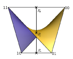
Figure 1: The binary independence model.

As a special case of the previous example, consider the binary independence model with $\mathcal{X}=\{00,01,10,11\}$,

$$A=\left(\begin{matrix}\smash{\overset{00}{1}}&\smash{\overset{01}{1}}&\smash{\overset{10}{0}}&\smash{\overset{11}{0}}\\ 0&0&1&1\\ 1&0&1&0\\ 0&1&0&1\end{matrix}\right),$$ (34)

and $r(x)=1$ for all $x\in\mathcal{X}$. It is easy to see that $\mathcal{E}$ consists of all probability measures $P$ which factorize as $P(x_{1}x_{2})=P_{1}(x_{1})P_{2}(x_{2})$, justifying the name of this model. The kernel is spanned by

$$u=(+1,-1,-1,+1),$$ (35)

corresponding to two global maximizers $P_{+}=\frac{1}{2}(\delta_{00}+\delta_{11})$ and $P_{-}=\frac{1}{2}(\delta_{01}+\delta_{10})$ (see figure 1).

7 Solving the critical equations

Finding the maximizers of $\overline{D}_{r}$ has some advantages over directly finding the maximizers of $D(\cdot||\mathcal{E})$, mainly because of two reasons:

1. The dimension of the problem is reduced: Instead of maximizing over the whole probability simplex the maximization takes place over a convex subset of the kernel of the matrix $A$. Therefore the dimension of the problem is reduced by the dimension of the exponential family.

2. A projection on the exponential family is not needed: $\overline{D}_{r}$ can be computed by a “simple” formula.

A numerical search for the maximizers using gradient search algorithms is now feasible for larger models. However, there may be a lot of local maximizers, so it is still a difficult problem to find the global maximizers of $D(\cdot||\mathcal{E})$. Of course, the above ideas can also be used with symbolic calculations in order to investigate the maximizers of $D(\cdot||\mathcal{E})$.

In the following assume that the sufficient statistics matrix $A$ has only integer entries. In this case the $\ker A$ has a basis of integer vectors. An important class of examples where this condition is satisfied are hierarchical models.

Under these assumptions we turn to the equations of Proposition 6. The main observation is that equation (29) is algebraic for suitable $u$ once we fix the sign vector of $u$. This motivates to look independently at each possible sign vector $\sigma$ that occurs in $\ker A$.

Remark 12.

Before investigating the critical equations some short remarks on the sign vectors are necessary. The set of possible sign vectors occuring in a vector space (in this case $\ker A$) forms a (realizable) oriented matroid. A sign vector $\sigma$ is called an (oriented) circuit if its support $\{x\in\mathcal{X}:\sigma_{x}\neq 0\}$ is inclusion minimal. See the first chapter of [5] for an introduction to oriented matroids.

Every sign vector can be written as a composition $\sigma_{1}\circ\dots\circ\sigma_{n}$ of circuits, where $\circ$ is the associative operation defined by

$$(\sigma_{i}\circ\sigma_{i+1})_{x}=\begin{cases}(\sigma_{i})_{x}&\text{ if }(\sigma_{i})_{x}\neq 0,\\ (\sigma_{i+1})_{x}&\text{ else }.\end{cases}$$ (36)

There is a free software package TOPCOM[16] which computes the signed circuits of a matrix. However, this package does not (yet) compute all the sign vectors, but this second step is easy to implement.

There is a second possible algorithm for computing all sign vectors of an oriented matroid, which shall only be sketched here, since it uses the complicated notion of duality (see [5] for the details): Namely, the set of all sign vectors is characterized by the so-called orthogonality property, meaning that the set of all sign vectors can be computed by calculating all cocircuits and checking the orthogonality property on each possible vector $\sigma\in\{0,\pm 1\}^{\mathcal{X}}$.

The nonzero sign vectors $\sigma$ occuring in a vector space always come in pairs $\pm\sigma$. It is customary to list only one representative of each such pair. This is not a problem, since the function $\overline{D}_{r}$ is antisymmetric, i.e., a local maximizer $u$ with sign vector $\operatorname{sgn}(u)=-\sigma$ corresponds to a local minimizer $-u$ with sign vector $\sigma$, and both will be quasi-critical points of $\overline{D}_{r}$.

Now fix a sign vector $\sigma$ and choose $u_{0}\in\ker A$ such that $\operatorname{sgn}(u_{0})=\sigma$ and $d_{u_{0}}=1$. Denote $\mathcal{Y}:=\operatorname{supp}(\sigma)=\operatorname{supp}(u_{0})$. Define $d^{\sigma}(v):=\sum_{x:\sigma_{x}>0}v(x)$. This implies $d^{\sigma}(v)=d^{\prime}_{u_{0}}(v)$ whenever $\operatorname{supp}(v)\subseteq\operatorname{supp}(u_{0})=\operatorname{supp}(\sigma)$. Let

$$K^{\sigma}:=\big{\{}v\in\ker A:d^{\sigma}(v)=0\text{ and }\operatorname{supp}(v)\subseteq\operatorname{supp}(\sigma)\big{\}}.$$ (37)

If $u\in\ker A$ satisfies $d_{u}=1$ and $\operatorname{sgn}(u)=\sigma$, then $u-u_{0}\in K^{\sigma}$. By definition $u$ is a quasi-critical point of $\overline{D}_{r}$ if and only if

$$\sum_{x\in\mathcal{Y}}v(x)\log\frac{|u(x)|}{r(x)}=0\text{ for all }v\in K^{\sigma}$$ (38)

(see Remark 9). These equations are linear in $v$, so it is enough to consider them for a spanning set of $K^{\sigma}$. Since by assumption the matrix $A$ has only integer entries the set

$$K^{\sigma}_{\mathbb{Z}}:=K^{\sigma}\cap\mathbb{Z}^{\mathcal{X}}$$ (39)

contains a spanning set of $K^{\sigma}$. Therefore $u$ is a quasi-critical point of $\overline{D}_{r}$ if and only if

$$\sum_{x\in\mathcal{Y}}v(x)\log\frac{|u(x)|}{r(x)}=0\text{ for all }v\in K^{\sigma}_{\mathbb{Z}}.$$ (40)

Exponentiating these equations gives

$$\prod_{x\in\mathcal{Y}:v(x)>0}\left(\frac{\sigma_{x}u(x)}{r(x)}\right)^{v(x)}=\prod_{x\in\mathcal{Y}:v(x)<0}\left(\frac{\sigma_{x}u(x)}{r(x)}\right)^{-v(x)}\text{ for all }v\in K^{\sigma}_{\mathbb{Z}}.$$ (41)

This is a system of polynomial equations. Every solution $u\in u_{0}+K^{\sigma}$ to this system that satisfies $\operatorname{sgn}(u)=\sigma$ is a quasi-critical point of $\overline{D}_{r}$ and thus a potential maximizer.

At this point it is possible to do one more simplification: If $v\in K_{\mathbb{Z}}^{\sigma}$, then $v(\sigma<0)=v(\sigma\neq 0)-v(\sigma>0)=0$. It follows that $v_{+}(\sigma<0)+v_{-}(\sigma<0)=0$, so

$$\prod_{x:v(x)>0}(\sigma_{x})^{v(x)}=(-1)^{v_{+}(\sigma<0)}=(-1)^{v_{-}(\sigma<0)}=\prod_{x:v(x)<0}(\sigma_{x})^{-v(x)}$$ (42)

All in all this yields:

Proposition 13.

Fix a sign vector $\sigma\in\{\pm 1\}^{\mathcal{X}}$. Let $u\in\ker A$ satisfy $d_{u}=1$ and

$$\prod_{x\in\mathcal{Y}}\left(\frac{u(x)}{r(x)}\right)^{v_{+}(x)}=\prod_{x\in\mathcal{Y}}\left(\frac{u(x)}{r(x)}\right)^{v_{-}(x)}$$ (43)

for all $v=v_{+}-v_{-}\in K_{\mathbb{Z}}^{\sigma}$. If $\operatorname{sgn}\left(u\right)=\sigma$, then $u$ is a quasi-critical point of $\overline{D}_{r}$. Every quasi-critical point of $\overline{D}_{r}$ arises in this way.

Remark 14.

Note that the system of equations (43) still contains infinitely many equations. The argument before equation (39) shows that a finite number of equations is enough. However, there are different possible choices for this finite set (at least a basis of $K_{\mathbb{Z}}^{\sigma}$ is needed), and the choice may have a large computational impact. This issue will be addressed below.

Proposition 13 shows that the maximizers of $\overline{D}_{r}$ can be found by analyzing all the solutions to the algebraic systems of equations (43) for all different possible sign vectors $\sigma$. Since the analysis of systems of polynomials works best over the complex numbers, in the following these equations will be considered as complex equations in the variables $u(x)$. Of course, only real solutions with the right sign pattern will be candidate solutions of the original maximization problem.

From now on fix $\sigma$ again. Define $I_{2}^{\sigma}\subseteq\mathbb{C}[u(x):x\in\mathcal{Y}]$ to be the ideal generated by all equations (43) in the polynomial ring $\mathbb{C}[u(x):x\in\mathcal{Y}]$ with one variable for each $x\in\mathcal{Y}$. Similarly, let $I_{1}^{\sigma}\subseteq\mathbb{C}[u(x):x\in\mathcal{Y}]$ be the ideal generated by the equations

$$\sum_{x\in\mathcal{Y}}A_{i,x}u(x)=0,\qquad\text{ for all }i.$$ (44)

Finally let $I^{\sigma}:=I_{1}^{\sigma}+I_{2}^{\sigma}$. The set of all common complex solutions of all equations in $I^{\sigma}$ is an algebraic subvariety of $\mathbb{C}^{\mathcal{Y}}$ and will be denoted by $X^{\sigma}$.

Remark 15.

Note that we omitted the equation $d_{u}-1=0$ in the definition of the ideal. It is easy to see that we can ignore this condition at first, because every solution satisfying $\operatorname{sgn}(u)=\sigma$ has $d(u)\neq 0$ and can thus be normalized to a solution with $d_{u}=1$. In other words, the original problem is solved once all points on the variety $X^{\sigma}$ that satisfy the sign condition are known. The algebraic reason for this fact is that all the defining equations of $I$ are homogeneous. This means that we can also replace $X^{\sigma}$ by the projective variety corresponding to $I^{\sigma}$, which is another interpretation of the fact that the normalization does not matter at this point.

Both ideals $I_{1}^{\sigma}$ and $I_{2}^{\sigma}$ taken for themselves are very nice: $I_{1}^{\sigma}$ corresponds to a system of linear equations, so it can be treated by the methods of linear algebra. On the other hand, $I_{2}^{\sigma}$ is a system of binomial equations, and there are a lot of theoretical results and fast algorithms for binomial equations[8, 11]. However, the sum of a linear ideal and a binomial ideal can be arbitrarily complicated. In fact, it is easy to see that any ideal can be reparameterized as a sum of a linear ideal and a binomial ideal: For example, a polynomial equation $\sum_{i}m_{i}=0$, where $m_{i}$ are arbitrary monomials, is equivalent to the system of equations

$$z_{i}-m_{i}=0,\text{ for all }i,$$

$$\sum_{i}z_{i}=0,$$

where one additional variable $z_{i}$ has been introduced for every monomial. Still, the two ideals $I_{1}^{\sigma}$ and $I_{2}^{\sigma}$ under consideration here are closely related, so there is hope that general statements can be made.

$X^{\sigma}$ equals the intersection of $X_{1}^{\sigma}$ and $X_{2}^{\sigma}$, where $X_{1}^{\sigma}$ and $X_{2}^{\sigma}$ are the varieties of $I_{1}^{\sigma}$ and $X_{2}^{\sigma}$ respectively. The variety $X_{1}^{\sigma}$ is easy to determine: By definition it is given by the (complex) kernel of $A$ restricted to $\mathcal{Y}$:

$$X_{1}^{\sigma}=\ker_{\mathbb{C}}A\cap\mathbb{C}^{\mathcal{Y}}.$$ (45)

The variety $X_{2}^{\sigma}$ is a little bit more complicated, but still a lot can be said.

By definition, $I_{2}^{\sigma}$ is generated by a countable collection of binomials. In fact, Hilbert’s Basissatz shows that a finite subset of the generators of $I_{2}^{\sigma}$ is sufficient to generate the ideal. In general it can be a difficult task to find such a finite subset, but since equations (43) correspond to directional derivatives, it is sufficient to consider them for any basis $B$ of $K^{\sigma}$ (see Remark 14). So denote the ideal generated by the equations corresponding to a basis $B$ of $\ker A$ by $I_{2}(B)$. In general $I_{2}(B)$ will have a different solution variety $V(I_{2}(B))$ than $I_{2}^{\sigma}$, and moreover $V(I_{2}(B))$ will depend on $B$. From what was said above all these varieties agree on the orthant of $\mathbb{R}^{\mathcal{X}}$ defined by $\operatorname{sgn}=\sigma$. The presence of additional (complex) solutions outside this orthant may complicate the algebraic analysis. It is obvious that all the ideals $I_{2}(B)$ are contained in $I_{2}^{\sigma}$. This means that $I_{2}^{\sigma}$ has the smallest solution set, so a finite generating set of $I_{2}^{\sigma}$ would be useful.

More precisely, since the ideal $I_{2}^{\sigma}$ is generated by binomials, the theory of [8] applies. Corollary 2.6 of this work implies that the ideal $I_{2}^{\sigma}$ is a prime ideal. This means that $X_{2}^{\sigma}$ is irreducible, i.e., it can not be written as a union of two proper subvarieties. Binomial prime ideals are also called toric ideals[8, remark before Corollary 2.6]. However, it is easy to construct examples such that $I_{2}(B)$ is not irreducible.

Fortunately there are fast computer algorithms, implemented in the software package 4ti2[1], which can be used to compute a finite generating set of $I_{2}^{\sigma}$ [10]. These algorithms compute finite generating sets of so-called lattice ideals. It turns out that $I_{2}^{\sigma}$ becomes a lattice ideal after a rescaling of the coordinates. To be concrete, writing $u_{r}(x):=\frac{u(x)}{r(x)}$ yields a new, equivalent ideal $I_{2,r}^{\sigma}\subseteq\mathbb{C}[u_{r}(x):x\in\mathcal{Y}]$ generated by the binomials

$$\prod_{x:v>0}u_{r}(x)^{v(x)}=\prod_{x:v<0}u_{r}(x)^{-v(x)},\quad\text{ for all }v\in K^{\sigma}_{\mathbb{Z}}.$$ (46)

The ideal $I_{2,r}^{\sigma}$ is called a lattice ideal, since it is related to the integer lattice $K^{\sigma}_{\mathbb{Z}}\subseteq\mathbb{Z}^{\mathcal{Y}}$.

Now we turn to $X^{\sigma}=X_{1}^{\sigma}\cap X_{2}^{\sigma}$. Even though $X_{1}^{\sigma}$ and $X_{2}^{\sigma}$ are irreducible, in general $X^{\sigma}$ will be reducible. This means that we can write $X^{\sigma}$ as a finite union of irreducible components $X^{\sigma}=V^{\sigma}_{1}\cup\dots\cup V^{\sigma}_{c}$. To each of these components $V^{\sigma}_{i}$ corresponds a polynomial ideal $I_{i}^{\sigma}$, and we have $u\in X^{\sigma}$ if and only if $u$ solves (at least) one of these ideals. The procedure to obtain the ideals $I_{i}^{\sigma}$ is called primary decomposition.

If an irreducible component $V^{\sigma}_{i}$ is zero-dimensional, then it consists of only one point, and it is easy to check whether this unique element $u\in X^{\sigma}_{i}$ satisfies $\operatorname{sgn}(u)=\sigma$. However, components of positive dimension may arise. In this case it is not easy to see whether these components contain elements $u$ satisfying $\operatorname{sgn}(u)=\sigma$. Fortunately, in many cases this information is not required:

Theorem 16.

Let $u$ be an element of an irreducible component $V$ of $X^{\sigma}$ such that $d_{\sigma}(u)=1$. Suppose there exists $u_{0}\in V$ such that $d_{\sigma}(u_{0})=1$ and $\operatorname{sgn}(u_{0})=\sigma$. Then

$$\overline{D}_{r}(u_{0})=\sum_{x\in\mathcal{Y}}\mathfrak{Re}(u(x))\log\frac{|u(x)|}{r(x)}.$$ (47)

Proof.

Let

$$V^{\prime}:=\{v\in V:v(x)\neq 0\text{ for all }x\in\mathcal{Y}\text{, and }d_{\sigma}(v)\neq 0\}.$$ (48)

Then $V^{\prime}$ is a Zariski-open subset of $V$, hence $V^{\prime}$ is irreducible. This implies that $V^{\prime}$ is pathconnected, so there exists a smooth path $\gamma:[0,1]\to V^{\prime}$ from $u$ to $u_{0}$. This is obvious if $V^{\prime}$ is regular, since then $V^{\prime}$ is a locally pathconnected and connected complex manifold. It follows that all regular points can be connected by a smooth path. Finally, every singular point $p$ can be linked by a smooth path to some regular point in any neighbourhood of $p$. By Remark 15 this path can be chosen such that $d_{\sigma}(\gamma_{t})=1$ for all $t\in[0,1]$.

Fix a point $u\in V^{\prime}$ and fix a convention for the logarithm. For every $x\in\mathcal{Y}$ the logarihm can be continued to a map $t\mapsto\log^{t,x}(\gamma_{t}(x))$. For every $t\in[0,1]$ define a linear functional $s_{t}:K^{\sigma}_{\mathbb{C}}\to\mathbb{C}$ via

$$s_{t}(v)=\frac{1}{2\pi i}\sum_{x\in\mathcal{Y}}v(x)\log^{t,x}\frac{\sigma_{x}\gamma_{t}(x)}{r(x)}.$$ (49)

By definition of $X^{\sigma}$ it follows that $s_{t}$ takes only integer values on $K^{\sigma}_{\mathbb{Z}}$, and $s_{t}$ can be identified with an element of the dual lattice $K^{\sigma*}_{\mathbb{Z}}$ of $K_{\mathbb{Z}}^{\sigma}$. Since $K_{\mathbb{Z}}^{\sigma*}$ is a discrete subset of the dual vector space $K_{\mathbb{C}}^{\sigma*}$ and since the map $t\mapsto s_{t}$ is continuous $s_{t}$ is constant along $\gamma$.

Now consider the function $f(t)=\sum_{x\in\mathcal{Y}}\gamma_{t}(x)\log^{t,x}\left(\frac{\sigma_{x}\gamma_{t}(x)}{r(x)}\right)$. Its derivative is $f^{\prime}(t)=\sum_{x\in\mathcal{Y}}\gamma^{\prime}_{t}(x)\log^{t,x}\left(\frac{\sigma_{x}\gamma_{t}(x)}{r(x)}\right)=2\pi is_{0}(\gamma^{\prime}_{t})$, where $\gamma^{\prime}_{t}(x)=\frac{\partial}{\partial t}\gamma_{t}(x)\in K_{\mathbb{Z}}^{\sigma}$. It follows that $f(1)-f(0)=2\pi is_{0}(\gamma_{1}-\gamma_{0})$. In other words,

$$\sum_{x\in\mathcal{Y}}u_{0}(x)\log^{1,x}\frac{\sigma_{x}u_{0}(x)}{r(x)}=\sum_{x\in\mathcal{Y}}u(x)\log\frac{\sigma_{x}u(x)}{r(x)}+2\pi is_{0}(u_{0}-u).$$ (50)

If $\log^{1,x}(\sigma_{x}u_{0}(x))=\log^{x}(\sigma_{x}u_{0}(x))+2\pi ik_{x}$ with $k_{x}\in\mathbb{Z}$, then

$$\overline{D}_{r}(u_{0})=f(0)+2\pi i\left(s_{0}(u_{0}-u)-\sum_{x\in\mathcal{Y}}u_{0}(x)k_{x}\right).$$ (51)

Taking the real parts of this equation gives

$$\overline{D}_{r}(u_{0}) =\mathfrak{Re}(f(0))+2\pi s_{0}(\mathfrak{Im}(u))$$

$$=\mathfrak{Re}(f(0))-i\sum_{x\in\mathcal{Y}}\mathfrak{Im}(u(x))\log\frac{\sigma_{x}u(x)}{r(x)}$$

$$=\mathfrak{Re}\left(\sum_{x\in\mathcal{Y}}\mathfrak{Re}(u(x))\log\frac{\sigma_{x}u(x)}{r(x)}\right)$$

$$=\sum_{x\in\mathcal{Y}}\mathfrak{Re}(u(x))\log\frac{|u(x)|}{r(x)}.$$

By continuity this formula continues to hold on the closure of $V^{\prime}$, which equals $V$. ∎

The theorem implies that in many cases only one point $u$ from each irreducible component of $X^{\sigma}$ needs to be tested. Only if $\sum_{x\in\mathcal{Y}}\mathfrak{Re}(u(x))\log\frac{|u(x)|}{r(x)}$ is exceptionally large it is necessary to analyze this irreducible component further and see if there is a real point $u_{0}$ from the same irreducible component that satisfies the sign condition.

Remark 17.

The above theorem also makes it possible to use methods of numerical algebraic geometry[17]. These methods can determine the number of irreducible components and their dimensions. Additionally it is possible to sample points from any irreducible component. In fact, each component is represented by a so-called witness set, a set of elements of this component. These points can then be used to numerically evaluate $\overline{D}_{r}$. One implementation, available on the Internet, is Bertini[4].

Let $x\in\mathcal{Y}$. For every irreducible component $X^{\sigma}_{i}$ there are the following alternatives:

• Either $u(x)=0$ for all $u\in X^{\sigma}_{i}$. In this case $\operatorname{sgn}(u)\neq\sigma$ on $X^{\sigma}_{i}$.

• Or $u(x)=0$ holds only on a subset of measure zero.

The reason for this is that the equation $u(x)=0$ defines a closed subset of $X^{\sigma}_{i}$, and either this closed subset is all of $X^{\sigma}_{i}$, or it has codimension one (this argument needs the irreducibility of $X^{\sigma}_{i}$).

When computing the primary decomposition the irreducible components of the first kind can be excluded algebraically by a method called saturation: Namely, the variety corresponding to the saturation

$$\left(I^{\sigma}:(\prod_{x\in\mathcal{Y}}u(x))^{\infty}\right)=\Big{\{}f\in\mathbb{C}[u(x)]:fm\in I^{\sigma}\text{ for some monomial }m\in\mathbb{C}[u(x)]\Big{\}}$$ (52)

consists only of those irreducible components of $X^{\sigma}$ which are not contained in any coordinate plane. In the same way we may also saturate by the polynomial $d^{\sigma}(M)$, since any solution $M$ with $\operatorname{sgn}(M)=\sigma$ will have $0\neq d(M)=d^{\sigma}(M)$.

The main reason why saturation is important is that it may reduce the complexity of symbolic calculations.

Example 18.

The above ideas can be applied to the hierarchical model (see [12]) of pair interactions among four binary random variables (the “binary 4-2 model”). This exponential family consists of all probability distributions of full support which factor as a product of functions that depend on only two of the four random variables.

The maximization problem of this model is related to orthogonal latin squares: If the binary random variables are replaced by random variables of size $k$, then the maximizer of the corresponding 4-2 model is easy to find if two orthogonal latin squares of size $k$ exist[14], and in this case the maximum value of $D(\cdot||\mathcal{E})$ equals $2\log(k)$. From this point of view, the following discussion will give an extremely complicated proof of the trivial fact that there are no two orthogonal latin squares of size two.

The sufficient statistics may be chosen as

$$A_{4-2}=\left(\begin{matrix}1\phantom{+}0\phantom{+}0\phantom{+}0\phantom{+}1\phantom{+}0\phantom{+}0\phantom{+}0\phantom{+}1\phantom{+}0\phantom{+}0\phantom{+}0\phantom{+}1\phantom{+}0\phantom{+}0\phantom{+}0\\ 0\phantom{+}1\phantom{+}0\phantom{+}0\phantom{+}0\phantom{+}1\phantom{+}0\phantom{+}0\phantom{+}0\phantom{+}1\phantom{+}0\phantom{+}0\phantom{+}0\phantom{+}1\phantom{+}0\phantom{+}0\\ 0\phantom{+}0\phantom{+}1\phantom{+}0\phantom{+}0\phantom{+}0\phantom{+}1\phantom{+}0\phantom{+}0\phantom{+}0\phantom{+}1\phantom{+}0\phantom{+}0\phantom{+}0\phantom{+}1\phantom{+}0\\ 1\phantom{+}0\phantom{+}1\phantom{+}0\phantom{+}0\phantom{+}0\phantom{+}0\phantom{+}0\phantom{+}1\phantom{+}0\phantom{+}1\phantom{+}0\phantom{+}0\phantom{+}0\phantom{+}0\phantom{+}0\\ 0\phantom{+}1\phantom{+}0\phantom{+}1\phantom{+}0\phantom{+}0\phantom{+}0\phantom{+}0\phantom{+}0\phantom{+}1\phantom{+}0\phantom{+}1\phantom{+}0\phantom{+}0\phantom{+}0\phantom{+}0\\ 0\phantom{+}0\phantom{+}0\phantom{+}0\phantom{+}1\phantom{+}0\phantom{+}1\phantom{+}0\phantom{+}0\phantom{+}0\phantom{+}0\phantom{+}0\phantom{+}1\phantom{+}0\phantom{+}1\phantom{+}0\\ 1\phantom{+}0\phantom{+}1\phantom{+}0\phantom{+}1\phantom{+}0\phantom{+}1\phantom{+}0\phantom{+}0\phantom{+}0\phantom{+}0\phantom{+}0\phantom{+}0\phantom{+}0\phantom{+}0\phantom{+}0\\ 0\phantom{+}1\phantom{+}0\phantom{+}1\phantom{+}0\phantom{+}1\phantom{+}0\phantom{+}1\phantom{+}0\phantom{+}0\phantom{+}0\phantom{+}0\phantom{+}0\phantom{+}0\phantom{+}0\phantom{+}0\\ 0\phantom{+}0\phantom{+}0\phantom{+}0\phantom{+}0\phantom{+}0\phantom{+}0\phantom{+}0\phantom{+}1\phantom{+}0\phantom{+}1\phantom{+}0\phantom{+}1\phantom{+}0\phantom{+}1\phantom{+}0\\ 1\phantom{+}1\phantom{+}0\phantom{+}0\phantom{+}0\phantom{+}0\phantom{+}0\phantom{+}0\phantom{+}1\phantom{+}1\phantom{+}0\phantom{+}0\phantom{+}0\phantom{+}0\phantom{+}0\phantom{+}0\\ 0\phantom{+}0\phantom{+}1\phantom{+}1\phantom{+}0\phantom{+}0\phantom{+}0\phantom{+}0\phantom{+}0\phantom{+}0\phantom{+}1\phantom{+}1\phantom{+}0\phantom{+}0\phantom{+}0\phantom{+}0\\ 0\phantom{+}0\phantom{+}0\phantom{+}0\phantom{+}1\phantom{+}1\phantom{+}0\phantom{+}0\phantom{+}0\phantom{+}0\phantom{+}0\phantom{+}0\phantom{+}1\phantom{+}1\phantom{+}0\phantom{+}0\\ 1\phantom{+}1\phantom{+}0\phantom{+}0\phantom{+}1\phantom{+}1\phantom{+}0\phantom{+}0\phantom{+}0\phantom{+}0\phantom{+}0\phantom{+}0\phantom{+}0\phantom{+}0\phantom{+}0\phantom{+}0\\ 0\phantom{+}0\phantom{+}1\phantom{+}1\phantom{+}0\phantom{+}0\phantom{+}1\phantom{+}1\phantom{+}0\phantom{+}0\phantom{+}0\phantom{+}0\phantom{+}0\phantom{+}0\phantom{+}0\phantom{+}0\\ 0\phantom{+}0\phantom{+}0\phantom{+}0\phantom{+}0\phantom{+}0\phantom{+}0\phantom{+}0\phantom{+}1\phantom{+}1\phantom{+}0\phantom{+}0\phantom{+}1\phantom{+}1\phantom{+}0\phantom{+}0\\ 1\phantom{+}1\phantom{+}1\phantom{+}1\phantom{+}0\phantom{+}0\phantom{+}0\phantom{+}0\phantom{+}0\phantom{+}0\phantom{+}0\phantom{+}0\phantom{+}0\phantom{+}0\phantom{+}0\phantom{+}0\\ 0\phantom{+}0\phantom{+}0\phantom{+}0\phantom{+}1\phantom{+}1\phantom{+}1\phantom{+}1\phantom{+}0\phantom{+}0\phantom{+}0\phantom{+}0\phantom{+}0\phantom{+}0\phantom{+}0\phantom{+}0\\ 0\phantom{+}0\phantom{+}0\phantom{+}0\phantom{+}0\phantom{+}0\phantom{+}0\phantom{+}0\phantom{+}1\phantom{+}1\phantom{+}1\phantom{+}1\phantom{+}0\phantom{+}0\phantom{+}0\phantom{+}0\\ 1\phantom{+}1\phantom{+}1\phantom{+}1\phantom{+}1\phantom{+}1\phantom{+}1\phantom{+}1\phantom{+}1\phantom{+}1\phantom{+}1\phantom{+}1\phantom{+}1\phantom{+}1\phantom{+}1\phantom{+}1\end{matrix}\right)$$

Here, the columns are ordered in such a way that the column number $i+1$ corresponds to the state $x_{i}\in\mathcal{X}=\{0,1\}^{4}$ that is indexed by the binary representation of $i\in\{0,\dots,15\}$.

The software package TOPCOM[16] is used to calculate the oriented circuits of $\ker A$, from which all sign vectors are computed by composition. Up to symmetry there are 73 different sign vectors occuring in $\ker A$. Here, the symmetry of the model is generated by the permutations of the four binary units and the relabelings $0\leftrightarrow 1$ of each unit.

From these 73 sign vectors only 20 satisfy condition 1. of Proposition 6. The sign vectors of small support are easy to handle: There are two sign vectors $\sigma_{1},\sigma_{2}$ whose support has cardinality eight. They are in fact oriented circuits, which implies that, up to normalization, there are two unique elements $u_{1},u_{2}\in\ker A$ such that $\operatorname{sgn}(u_{i})=\sigma_{i}$, $i=1,2$. They satisfy $\overline{D}_{r}(u_{i})=0$, so they are surely not global maximizers.

There are three sign vectors whose support has cardinality twelve. Let $\sigma$ be one of these. Then the restriction $\operatorname{supp}(u)\subseteq\operatorname{supp}(\sigma)$ selects a two-dimensional subspace of $\ker A$, and it is easy to see that $\overline{D}_{r}=0$ on this subspace.

There remain 15 sign vectors that have a full support. For every such sign vector $\sigma$ the system of the algebraic equations in $I_{1}^{\sigma}$ and $I_{2}^{\sigma}$ has to be solved. To reduce the number of equations and the number of variables one may parametrize the solution set $\ker_{\mathbb{C}}A$ of $I_{1}^{\sigma}$ by finding a basis $u_{1},\dots,u_{5}$ of $\ker A$. Then this parametrization is plugged into the equations of $I_{2}^{\sigma}$. Some of these systems are at the limit of what today’s desktop computer can handle. Therefore care has to be taken how to formulate these equations. The general strategy is the following:

1. At first, compute a basis $v_{1},\dots,v_{k-1}$ of $K_{\mathbb{Z}}^{\sigma}$ by using a Gram-Schmidt-like algorithm: Renumber the $u_{i}$ such that $d_{\sigma}(u_{5})\neq 0$ and let

   $$v_{i}:=\frac{d_{\sigma}(u_{5})}{g}u_{i}-\frac{d_{\sigma}(u_{i})}{g}u_{5},$$ (53)

   where $g=\gcd(d_{\sigma}(u_{5}),d_{\sigma}(u_{i}))$.

2. Let $I$ be the ideal in the variables $\lambda_{1},\dots,\lambda_{5}$ generated by the equations

   $$\prod_{x:v_{i}>0}u(x)^{v_{i}(x)}-\prod_{x:v_{i}<0}u(x)^{-v_{i}(x)},\text{ for all }i=1,\dots,4,$$ (54)

   where $u(x)=\sum_{i=1}^{5}\lambda_{i}u_{i}(x)$.

3. Compute the saturation $J=(I:\prod_{x\in\mathcal{X}}u(x)^{\infty})$.

4. Compute the primary decomposition of $J$.

Note that the ideal $I$ in the second step corresponds to the ideal $I_{2}(B)$ defined above for the basis $B=\{v_{1},\dots,v_{4}\}$, where the variables $u(x)$ have been restricted to the linear subspace $\ker_{\mathbb{C}}A$. The ideal $J$ obtained by saturation in the third step is then independent of $B$.

Unfortunately, this simple algorithm does not work for all sign vectors. Some further tricks are needed to compute the primary decomposition within a reasonable time.

A basis of $\ker A$ is given by the rows $u_{1},\dots,u_{5}$ of the matrix

$$\left(\begin{matrix}\;1\phantom{+}{-1}\phantom{+}{-1}\phantom{+}\phantom{-}1\phantom{+}{-1}\phantom{+}\phantom{-}1\phantom{+}\phantom{-}1\phantom{+}{-1}\phantom{+}{-1}\phantom{+}\phantom{-}1\phantom{+}\phantom{-}1\phantom{+}{-1}\phantom{+}\phantom{-}1\phantom{+}{-1}\phantom{+}{-1}\phantom{+}\phantom{-}1\\ \;1\phantom{+}\phantom{-}0\phantom{+}{-1}\phantom{+}\phantom{-}0\phantom{+}{-1}\phantom{+}\phantom{-}0\phantom{+}\phantom{-}1\phantom{+}\phantom{-}0\phantom{+}{-1}\phantom{+}\phantom{-}0\phantom{+}\phantom{-}1\phantom{+}\phantom{-}0\phantom{+}\phantom{-}1\phantom{+}\phantom{-}0\phantom{+}{-1}\phantom{+}\phantom{-}0\\ \;1\phantom{+}{-1}\phantom{+}\phantom{-}0\phantom{+}\phantom{-}0\phantom{+}{-1}\phantom{+}\phantom{-}1\phantom{+}\phantom{-}0\phantom{+}\phantom{-}0\phantom{+}{-1}\phantom{+}\phantom{-}1\phantom{+}\phantom{-}0\phantom{+}\phantom{-}0\phantom{+}\phantom{-}1\phantom{+}{-1}\phantom{+}\phantom{-}0\phantom{+}\phantom{-}0\\ \;1\phantom{+}{-1}\phantom{+}{-1}\phantom{+}\phantom{-}1\phantom{+}\phantom{-}0\phantom{+}\phantom{-}0\phantom{+}\phantom{-}0\phantom{+}\phantom{-}0\phantom{+}{-1}\phantom{+}\phantom{-}1\phantom{+}\phantom{-}1\phantom{+}{-1}\phantom{+}\phantom{-}0\phantom{+}\phantom{-}0\phantom{+}\phantom{-}0\phantom{+}\phantom{-}0\\ \;1\phantom{+}{-1}\phantom{+}{-1}\phantom{+}\phantom{-}1\phantom{+}{-1}\phantom{+}\phantom{-}1\phantom{+}\phantom{-}1\phantom{+}{-1}\phantom{+}\phantom{-}0\phantom{+}\phantom{-}0\phantom{+}\phantom{-}0\phantom{+}\phantom{-}0\phantom{+}\phantom{-}0\phantom{+}\phantom{-}0\phantom{+}\phantom{-}0\phantom{+}\phantom{-}0\end{matrix}\right).$$

This basis has the following property: Let $u=\sum_{i=1}^{5}\lambda_{i}u_{i}$. If $\lambda_{j}=0$ for some $j=2,3,4,5$, then $\overline{D}(u)=0$. The reason is that if one $\lambda_{j}$ vanishes, then it is easy to see that there is bijection between the positive and negative entries of $u$ such that corresponding entries have the same absolute value. This implies that, in order to determine the global maximizer of this model one may saturate $J$ by the product $\lambda_{2}\lambda_{3}\lambda_{4}\lambda_{5}$.

Replacing $J$ by $\left(J:(\lambda_{2}\lambda_{3}\lambda_{4}\lambda_{5})^{\infty}\right)$ makes it possible to solve all but one system of equations. For the last sign vector $\sigma$ a special measure is necessary: The complexity of the above algorithm depends on the chosen basis $v_{1},v_{2},v_{3},v_{4}$ of $K^{\sigma}_{\mathbb{Z}}$. The $\ell_{1}$-norm of each vector $v_{i}$ equals twice the degree of the corresponding equation. Thus it is advisable to choose the vectors $v_{1},v_{2},v_{3},v_{4}$ as short as possible. As a first approximation, one may try to use a basis of circuit vectors, i.e., vectors whose support is minimal. This approach provides a basis $v_{1},v_{2},v_{3},v_{4}$ for $K_{\mathbb{Z}}^{\sigma}$ of the last sign vector, such that the rest of the algorithm sketched above works.

The calculations were performed with the help of Singular[9]. The primary decompositions were done using the algorithm of Gianni, Trager and Zacharias (GTZ) implemented in the library solve.lib. Analyzing the results yields the following theorem, confirming a conjecture by Thomas Kahle (personal communication):

Theorem 19.

The binary 4-2 model has, up to symmetry, a unique maximizer of the information divergence, which is the uniform distribution over the states $0001$, $0010$, $0100$, $1000$ and $1111$. The maximal value of $\overline{D}$ is $\log 3-\frac{1}{3}\log 5\approx 0.56213298$, it is reached at

$$u=\frac{1}{15}(-5,3,3,-1,3,-1,-1,-1,3,-1,-1,-1,-1,-1,-1,3).$$ (55)

The maximum value of the $D(\cdot||\mathcal{E})$ is $=\log(1+3\cdot 5^{\frac{1}{3}})\approx 1.0132035$.

8 Computing the projection points

The theory of this paper motivates a second method for computing the maximizers of $D(\cdot||\mathcal{E})$, which is more elementary than solving the critical equations. However, knowing the critical equations sheds new light on this method.

Let $P_{+}$ be a projection point and construct $P_{-}$ as in section 3. Then $u=P_{+}-P_{-}$ and the common $rI$-projection $P_{\mathcal{E}}$ of $P_{+}$ and $P_{-}$ satisfy

$$u(x)=\begin{cases}\frac{1}{\mu}P_{\mathcal{E}}(x)&\text{ if }x\in\mathcal{Z},\\ -\frac{1}{1-\mu}P_{\mathcal{E}}(x)&\text{ if }x\notin\mathcal{Z}.\end{cases}$$ (56)

On the other hand, $P_{\mathcal{E}}$ lies in the closure of the exponential family. Suppose that $P_{\mathcal{E}}$ has full support. Then the exponential parameterization (1) implies that there exist $\alpha_{1},\dots,\alpha_{h}>0$

$$P_{\mathcal{E}}(x)=\frac{r(x)}{Z_{\alpha}}\prod_{i=1}^{h}\alpha_{i}^{A_{i,x}}.$$ (57)

Assume that $\sigma=\operatorname{sgn}(P_{+}-P_{-})$ has full support and define a $(h+1)\times\mathcal{X}$-matrix $A^{\sigma}$ as follows: Take the matrix $A$ and add a zeroth row with entries

$$A^{\sigma}_{0,x}:=1-\sigma_{x}\in\{0,1\}.$$ (58)

Then equations (56) and (57) together show that $u$ has the form

$$u(x)=r(x)\prod_{i=0}^{h}\alpha_{i}^{A^{\sigma}_{i,x}}$$ (59)

for suitably chosen $\alpha_{i}$. Here, $\alpha_{0}=-\frac{\mu}{1-\mu}<0$, and all the other parameters are positive. The normalization can be achieved since the row span of $A$ contains the constant vector. Thus the projection points, which project into $\mathcal{E}$, can be found by plugging the parameterization (59) into the equation $Au=0$ and solving for the $\alpha_{i}$.

Again, this method simplifies if $A$ has only integer entries. Additionaly it is convenient to suppose that $A$ has only nonnegative entries. This nonnegativity requirement can always be supposed, since $A$ contains the constant row in its row span. In this case the parameterization (59) is monomial, so the equation $Au=0$ is equivalent to $h$ polynomial equations in the $h+1$ parameters $\alpha_{0},\dots,\alpha_{h}$.

This method is linked to the ideal $I_{2}^{\sigma}$ of the previous section. As stated there, $I_{2}^{\sigma}$ is related to the lattice ideal $I_{2,r}^{\sigma}$, which defines a toric variety. Every toric variety has a monomial “parameterization”, which induces the monomial parameterization (59). Unfortunately, in the general case this monomial parameterization is not surjective. However, equation (59) shows that it is “surjective enough”, at least in the case where $\sigma$ has full support.

It is possible to extend this analysis to the case where $\sigma$ does not have full support. Let $\mathcal{Y}=\operatorname{supp}(\sigma)$. First it is necessary to parameterize the set $\mathcal{E}^{\mathcal{Y}}$ of those probability distributions of $\overline{\mathcal{E}}$ whose support is $\mathcal{Y}$. One solution is to find an element $r_{\mathcal{Y}}\in\overline{\mathcal{E}}$ such that $\operatorname{supp}(r_{\mathcal{Y}})=\mathcal{Y}$. Then $\mathcal{E}^{\mathcal{Y}}$ equals the exponential family over the set $\mathcal{Y}$ with reference measure $r_{\mathcal{Y}}$ whose sufficient statistics matrix $A_{\mathcal{Y}}$ consists of those columns of $A$ corresponding to $\mathcal{Y}\subseteq\mathcal{X}$. This gives a monomial parameterization of $\mathcal{E}^{\mathcal{Y}}$ with at most $h$ parameters.

The equations obtained from $Au=0$ by plugging in a monomial parameterization for $u$ can be solved by primary decomposition. Every solution $(\alpha_{0},\dots,\alpha_{h})$ yields a point of $X^{\sigma}$. Theorem 16 applies in this context.

Example 20.

The above ideas can be used to find the maximizers of the independence model of three random variables of cardinalities 2, 3 and 3. This example is particularly interesting, since the global maximizers are known for those independence models where the cardinality of the state spaces of the random variables satisfy an inequality[3]. The cardinalities 2, 3 and 3 are the smallest set of cardinalities that violate this inequality.

A sufficient statistics of the model is given by

$$A_{2-3-3}=\left(\begin{tabular}[]{*{18}{c}}1&1&1&1&1&1&1&1&1&1&1&1&1&1&1&1&1&1\\ 1&0&0&1&0&0&1&0&0&1&0&0&1&0&0&1&0&0\\ 0&1&0&0&1&0&0&1&0&0&1&0&0&1&0&0&1&0\\ 1&1&1&0&0&0&0&0&0&1&1&1&0&0&0&0&0&0\\ 0&0&0&1&1&1&0&0&0&0&0&0&1&1&1&0&0&0\\ 1&1&1&1&1&1&1&1&1&0&0&0&0&0&0&0&0&0\end{tabular}\right).$$ (60)

The states are numbered in the ternary representation from $000$ to $122$, where the “highest” random variable only takes two values. The dimension of the model is $d=5$ and the state space has cardinality 18. Thus $\dim\ker A=18-5-1=12$. The symmetry group of the model is generated by the permutation of the two random variables of cardinality three and by the permutations within the state space of each random variable.

The cocircuits can be computed by TOPCOM. Testing all $3^{18}$ possible sign vectors of length 18 shows that there are $182\,796$ non-zero sign vectors in $\ker A$ (up to symmetry). Checking the support condition 1. leaves 975 sign vectors. Excluding all sign vectors where the support of both the negative and the positive part exceeds 6 (cf. Theorem B) reduces the problem to 240 sign vectors.

The 72 sign vectors that do not have full support can be treated as in the previous section. For the 168 sign vectors that have full support the corresponding systems of equations consist of $\dim\ker A-1=11$ equations of $\dim\ker A=12$ variables. These are too difficult to solve in this way, but they can be treated using the method proposed in this section, which “only” requires the primary decomposition of a system of $d=5$ polynomials in $d+1=6$ variables.

The analysis was carried out with the help of Singular. It proved to be advantageous to use the algorithm of Shimoyama and Yokoyama (SY) from the library solve.lib. The following result was obtained:

Theorem 21.

The maximal value of $D(\cdot||\mathcal{E})$ for the independence model of cardinalities 2, 3 and 3 equals $\log(3+2\sqrt{2})\approx 1.7627472$, and the maximal value of $\overline{D}_{r}$ is $\log(2(1+\sqrt{2}))\approx 1.5745208$. Up to symmetry there is a unique global maximizing probability distribution

$$(1-\frac{\sqrt{2}}{2})(\delta_{012}+\delta_{020})+(\sqrt{2}-1)\delta_{100}.$$ (61)

In order to compare the two methods of finding the maximiers of $\overline{D}_{r}$ resp. $D(\cdot||\mathcal{E})$ presented in this section and in the last section let $d$ be the dimension of the model and let $r=\dim\ker A$. All algorithms are most efficient if $A$ is chosen such that $h=d+1$. Then, for any sign vector $\sigma$ with full support, the algorithm on page 18 starts with $r-1$ equations (corresponding to a basis of $K_{\mathbb{C}}^{\sigma}$) in $r$ variables $\lambda_{1},\dots,\lambda_{r}$, which are then saturated. On the other hand, the method in this section starts with the $d+1$ equations $Au=0$ in the $d+2$ variables $\alpha_{0},\dots,\alpha_{d+1}$. Thus, generically, the first method should perform better when the codimension of the model is small, while the second method should perform better when the dimension of the model is small.

9 Conclusions

In this work a new method for computing the maximizers of the information divergence from an exponential family $\mathcal{E}$ has been presented. The original problem of maximizing $D(\cdot||\mathcal{E})$ over the set of all probability distributions is transformed into the maximization of a function $\overline{D}_{r}$ over $\ker A$, where $A$ is the sufficient statistics of $\mathcal{E}$. It has been shown that the global maximizers of both problems are equivalent. Furthermore, every local maximizer of $D(\cdot||\mathcal{E})$ yields a maximizer of $\overline{D}_{r}$. At present it is not known whether the converse statement also holds.

The two main advantages of the reformulation are:

1. A reduction of the dimension of the problem.

2. The function $\overline{D}_{r}$ can be computed by a formula.

If $\mathcal{E}$ has codimension one, then the first advantage is most visible. Even this simple case can be useful in order to obtain examples of maximizers having specific properties.

The maximizers of $\overline{D}_{r}$ can be computed by solving the critical equations. These equations are nice if they are considered separately for every sign vector $\sigma$ occuring in $\ker A$. There are some conditions which allow to exclude certain sign vectors from the beginning. If the matrix $A$ contains only integer entries, then the critical equations are algebraic, once the sign vector is fixed. In this case tools from commutative algebra can be used to solve these equations.

A second possibility is to compute the points satisfying the projection property. If $A$ is an integer matrix and if the sign vector is fixed, then one obtains algebraic equations which are related to the critical equations of $\overline{D}$. This method is more appropriate for exponential families of small dimension.

Of course, a problem with these two approaches is that every sign vector needs to be treated separately, and their number grows quickly. By contrast, the problem of finding the maximizers of $D(\cdot||\mathcal{E})$ becomes a smooth problem if one restricts the support of the possible maximizers. In general the set of possible support sets is much smaller than the set of sign vectors. Still, two examples have been given where the maximizers where not known before and where the separate analysis of each sign vector was feasible.

References

- [1] 4ti2 team. 4ti2—a software package for algebraic, geometric and combinatorial problems on linear spaces. Available at www.4ti2.de.
- [2] Nihat Ay. An information-geometric approach to a theory of pragmatic structuring. Annals of Probability, 30:416–436, 2002.
- [3] Nihat Ay and Andreas Knauf. Maximizing multi-information. Kybernetika, 42:517–538, 2006.
- [4] Daniel J. Bates, Jonathan D. Hauenstein, Andrew J. Sommese, and Charles W. Wampler. Bertini: software for numerical algebraic geometry. Available at http://www.nd.edu/sommese/bertini.
- [5] A. Björner, M. Las Vergnas, B. Sturmfels, N. White, and G. Ziegler. Oriented matroids. Encyclopedia of Mathematics and its Applications. Cambridge, 1993.
- [6] David A. Cox, John B. Little, and Don O’Shea. Ideals, varieties, and algorithms: an introduction to computational algebraic geometry and commutative algebra. Springer, 2008.
- [7] Imre Csiszár and Paul C. Shields. Information theory and statistics: a tutorial. Foundations and Trends in Communications and Information Theory. now Publishers, 2004.
- [8] David Eisenbud and Bernd Sturmfels. Binomial ideals. Duke Mathematical Journal, 84(1):1–45, 1996.
- [9] G.-M. Greuel, G. Pfister, and H. Schönemann. Singular 3-1-0 — A computer algebra system for polynomial computations. Available at http://www.singular.uni-kl.de, 2009.
- [10] Raymond Hemmecke and Peter Malkin. Computing generating sets of lattice ideals. Journal of Symbolic Computation, 2009. accepted.
- [11] Thomas Kahle. Decomposition of binomial ideals. AISM, 2009. submitted.
- [12] Steffen L. Lauritzen. Graphical models. Oxford Statistical Science Series. Oxford University Press, 1996.
- [13] František Matúš. Optimality conditions for maximizers of the information divergence from an exponential family. Kybernetika, 43(5):731–746, 2007.
- [14] František Matúš. Divergence from factorizable distributions and matroid representations by partitions. IEEE Trans. Inform. Theory, 55:5375–5381, 2009.
- [15] František Matúš and Nihat Ay. On maximization of the information divergence from an exponential family. In Proceedings of the WUPES’03, pages 199–204. University of Economics, Prague, 2003.
- [16] Jörg Rambau. TOPCOM: Triangulations Of Point Configurations and Oriented Matroids. In Arjeh M. Cohen, Xiao-Shan Gao, and Nobuki Takayama, editors, Mathematical Software—ICMS 2002, pages 330–340. World Scientific, 2002.
- [17] Andrew J. Sommese and Charles W. Wampler. The numerical solution of systems of polynomials arising in engineering and science. World Scientific Publishing Company, 2005.