Probability Density in the Complex Plane

Abstract

The correspondence principle asserts that quantum mechanics resembles classical mechanics in the high-quantum-number limit. In the past few years many papers have been published on the extension of both quantum mechanics and classical mechanics into the complex domain. However, the question of whether complex quantum mechanics resembles complex classical mechanics at high energy has not yet been studied. This paper introduces the concept of a local quantum probability density $\rho(z)$ in the complex plane. It is shown that there exist infinitely many complex contours $C$ of infinite length on which $\rho(z)\,dz$ is real and positive. Furthermore, the probability integral $\int_{C}\rho(z)\,dz$ is finite. Demonstrating the existence of such contours is the essential element in establishing the correspondence between complex quantum and classical mechanics. The mathematics needed to analyze these contours is subtle and involves the use of asymptotics beyond all orders.

I Introduction

In conventional quantum mechanics, operators such as the Hamiltonian $\hat{H}$ and the position $\hat{x}$ are ordinarily taken to be real in the sense that they are Hermitian (${\hat{H}}={\hat{H}}^{\dagger}$). The condition of Hermiticity allows the matrix elements of these operators to be complex, but guarantees that their eigenvalues are real. Similarly, in the study of classical mechanics the trajectories of particles are assumed to be real functions of time. However, in recent years both quantum mechanics and classical mechanics have been extended and generalized to the complex domain. In classical dynamical systems the complex as well as the real solutions to Hamilton’s differential equations of motion have been studied C1 ; C2 ; C3 ; C4 ; C5 ; C6 ; C7 ; C8 ; C9 ; D1 ; D2 ; D3 ; D4 ; D5 ; D6 ; D7 ; D8 ; D9 ; D10 . In this generalization of conventional classical mechanics, classical particles are not constrained to move along the real axis and may travel through the complex plane. In quantum mechanics the class of physically allowed Hamiltonians has been broadened to include non-Hermitian ${\cal P}{\cal T}$-symmetric Hamiltonians in addition to Hermitian Hamiltonians, and wave functions (solutions to the Schrödinger equation) are treated as functions of complex coordinates C1 ; E1 ; E2 ; E3 ; E4 ; E5 ; E6 ; E7 ; E8 ; E9 . Experimental observations of physical systems described by complex ${\cal P}{\cal T}$-symmetric Hamiltonians are now being reported FF1 ; FF2 ; FF3 ; FF4 ; S6 ; S7 ; S8 ; S9 .

The relationship between quantum mechanics and classical mechanics is subtle. Quantum mechanics is essentially wavelike; probability amplitudes are described by a wave equation and physical observations involve such wavelike phenomena as interference patterns and nodes. In contrast, classical mechanics describes the motion of particles and exhibits none of these wavelike features. Nevertheless, there is a connection between quantum mechanics and classical mechanics, and according to Bohr’s famous correspondence principle this subtle connection becomes more pronounced at high energy.

Pauling and Wilson H1 give a simple pictorial explanation of the correspondence principle and this explanation is commonly repeated in other standard texts on quantum mechanics (see, for example, Ref. H2 ). One compares the probability densities for a quantum and for a classical particle in a potential well. For the harmonic-oscillator Hamiltonian

$$H=p^{2}+x^{2}$$ (1)

the quantum energy levels are $E_{n}=2n+1$ ($n=0,\,1,\,2,\,3,\,\ldots$). The fourth eigenfunction $\psi_{4}(x)$ has four nodes, and the associated probability density $\rho(x)=|\psi_{4}(x)|^{2}$ also has four nodes (see Fig. 1). When $n=16$, the quantum probability density has 16 nodes (see Fig. 2). The probability density for a classical particle is inversely proportional to the speed of the particle and is thus a smooth nonoscillatory curve, while the quantum-mechanical probability density is oscillatory and has nodes. Figures 1 and 2 show that the classical probability at high energy is a local average of the quantum probability. (The nature of this averaging process can be studied by performing a semiclassical approximation of the quantum-mechanical wave function. However, we do not discuss semiclassical approximations here.)

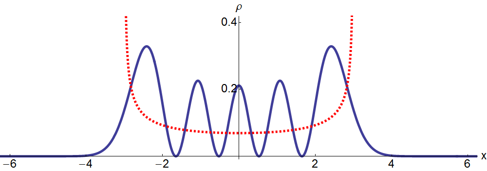
Figure 1: Graphical illustration of the correspondence principle. This figure compares the probability densities for a quantum and for a classical particle in a parabolic potential. The normalized quantum-mechanical probability density $\rho(x)=|\psi_{4}(x)|^{2}$ for a quantum particle of energy $E_{4}=9$ is plotted as a function of $x$ (solid curve); $\rho(x)$ is wavelike and exhibits four nodes. The normalized classical probability density for a particle of the same energy is also plotted (dotted curve); the classical probability density is not wavelike. Both probability densities are greatest near the turning points, which lie at $\pm 3$, because the speed of the particle is smallest in the vicinity of the turning points. Thus, the particle spends most of its time and is most likely to be found near the turning points. The classical probability density, which is the inverse of the speed $s$ of the particle, is infinite at the turning points because $s$ vanishes at the turning points, but this singularity is integrable.

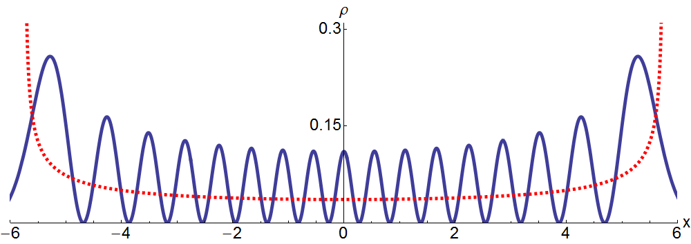
Figure 2: Comparison of the normalized probability densities for a quantum particle and for a classical particle of energy $E_{16}=33$ in a parabolic potential. The quantum probability density (solid curve) has 16 nodes and is wavelike while the classical probability density (dotted curve) is not wavelike; inside the potential well the quantum density oscillates about the classical density.

The objective of this paper is to extend and expand the work in a recent letter that examines the relationship between complex classical mechanics and complex quantum mechanics I0 . In particular, we show how to generalize the elementary Pauling-and-Wilson picture of the correspondence principle into the complex domain. We will see that in the complex domain some of the distinctions between classical mechanics and quantum mechanics become less pronounced. For example, in complex classical mechanics, particle trajectories can enter classically forbidden regions and consequently exhibit tunneling-like phenomena I1 ; I2 .

Figures 1 and 2 highlight an important difference between real classical systems and real quantum systems in the classically forbidden region: Outside the classically allowed region, which is delimited by the turning points, the classical probability density vanishes identically while the quantum-mechanical probability density is nonzero and decays exponentially. This discrepancy decreases as the energy increases because the quantum probability becomes more localized in the classically allowed region, but for any value of the energy there remains a sharp cutoff in the classical probability beyond the turning points.

In the physical world the cutoff at the boundary between the classically allowed and the classically forbidden regions is not perfectly sharp. For example, in classical optics it is known that below the surface of an imperfect conductor, the electromagnetic fields do not vanish abruptly. Rather, they decay exponentially as functions of the penetration depth. This effect is known as skin depth H3 . The case of total internal reflection is similar: When the angle of incidence is less than a critical angle, there is a reflected wave and no transmitted wave. However, the electromagnetic field does cross the boundary; this field is attenuated exponentially in a few wavelengths beyond the interface. Although this field does not vanish in the classically forbidden region, there is no flux of energy; that is, the Poynting vector vanishes in the classically forbidden region beyond the interface.

When classical mechanics is extended into the complex domain, classical particles are allowed to enter the classically forbidden region. However, in the forbidden region there is no particle flow parallel to the real axis. Rather, the flow of classical particles is orthogonal to the axis. This feature is analogous to the vanishing flux of energy in the case of total internal reflection as described above.

We illustrate these properties of complex classical mechanics by using the classical harmonic oscillator, whose Hamiltonian is given in (1). The classical equations of motion are

$$\dot{x}=2u,\quad\dot{y}=2v,\quad\dot{u}=-2x,\quad\dot{v}=-2y,$$ (2)

where the complex coordinate is $x+iy$ and the complex momentum is $u+iv$. For a particle having real energy $E$ and initial position $x(0)=a>\sqrt{E}$, $y(0)=0$, the solution to (2) is

$$x(t)=a\cos(2t),\quad y(t)=\sqrt{a^{2}-E}\sin(2t).$$ (3)

Thus, the possible classical trajectories are a family of ellipses parametrized by the initial position $a$:

$$\frac{x^{2}}{a^{2}}+\frac{y^{2}}{a^{2}-E}=1.$$ (4)

Four of these trajectories are shown in Fig. 3. Each trajectory has the same period $T=\pi$. The degenerate ellipse, whose foci are the turning points at $x=\pm\sqrt{E}$, is the familiar real solution. Note that classical particles may visit the real axis in the classically forbidden regions $|x|>\sqrt{E}$, but that the elliptical trajectories are orthogonal rather than parallel to the real axis.

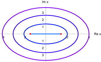
Figure 3: Classical trajectories in the complex plane for the harmonic-oscillator Hamiltonian (1). These trajectories are nested ellipses. Observe that when the harmonic oscillator is extended into the complex domain, the classical particles may pass through the classically forbidden regions outside the turning points. When the trajectories cross the real axis, they are orthogonal to it.

We can use the solution in (3) to extend the plots of classical probabilities in Figs. 1 and 2 to the complex plane. The speed $s$ of a classical particle at the complex coordinate point $x+iy$ is given by

$$s(x,y)=\left(E^{2}+x^{4}+y^{4}+2x^{2}y^{2}+2y^{2}E-2x^{2}E\right)^{1/4}.$$ (5)

If we assume that all ellipses are equally likely trajectories, then the relative probability density of finding the classical particle at the point $x+iy$ is $1/s(x,y)$. This function is plotted in Fig. 4. Figure 4 shows that the classical-mechanical probability density extends beyond the classically allowed region and into the complex plane. In this figure the distribution of classical probability in the complex plane falls off as the reciprocal of the distance from the origin. Thus, beyond the turning points on the real line the classical probability density is no longer identically zero, and what is more, it begins to resemble the quantum-mechanical probability density in the classically forbidden regions on the real axis in Figs. 1 and 2.

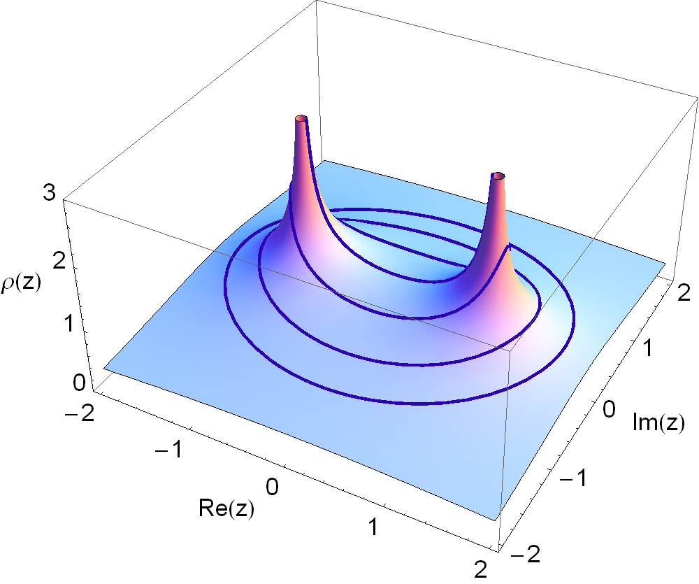
Figure 4: Classical-mechanical relative probability density for finding a particle at a point $x+iy$ in the complex plane for a particle subject to harmonic forces. The probability density resembles a pup tent with infinitely high tent poles located at the turning points. The complex classical ellipses in Fig. 3 are superposed on the tent canopy.

We emphasize that while the probability surface in Fig. 4 has the feature that it does not vanish on the real axis in the classically forbidden regions, it is entirely classical and thus there is none of the wavelike behavior that one would expect in quantum mechanics. This plot is two-dimensional and not one-dimensional, and this motivates us to define and calculate the complex analog of the quantum-mechanical probability density $\rho(z)$ in the complex-$z$ plane. As in conventional quantum mechanics, this probability density $\rho$ depends quadratically on the wave function $\psi$, and by virtue of the time-dependent Schrödinger equation, $\rho$ satisfies a local conservation law in the complex plane.

Extending the quantum-mechanical probability density into the complex plane is nontrivial because $\psi(z)$ is a complex-valued function of $z$, and as we will see, $\rho(z)$ is not the absolute square of $\psi$ and thus $\rho(z)$ is also a complex-valued function. In contrast with ordinary quantum theory, it is not clear whether $\rho(z)$ can be interpreted as a physical local probability density. To solve this problem we identify special curves in the complex-$z$ plane on which $\rho(z)dz$ is real and positive. We find these special curves by constructing a differential equation that these curves obey. Discovering these curves then allows us to formulate the complex version of the correspondence principle.

The complex correspondence principle is extremely delicate; understanding the probability density in complex quantum mechanics requires sophisticated mathematical tools, including the use of asymptotic analysis beyond Poincaré asymptotics; that is, asymptotic analysis of transcendentally small contributions. This paper is organized as follows: In Sec. II we obtain the form of the complex probability density in complex ${\cal P}{\cal T}$ quantum mechanics and discuss the specific case of the harmonic oscillator. Then, in Sec. III we give a simple example of a complex system, namely, a random walk with a complex bias, that has a real probability distribution in the complex plane. Next, in Sec. IV we study the special case of the complex probability for the ground state of the quantum harmonic oscillator. In Sec. V we consider the complex probability for the excited states of the harmonic oscillator. The quasi-exactly-solvable ${\cal P}{\cal T}$-symmetric anharmonic oscillator is discussed in Sec. VI. Finally, in Sec. VII we give some concluding remarks and discuss future directions for research.

II Local conservation law and probability density in the complex domain

In this section we derive a local conservation law associated with the time-dependent Schrödinger equation for a complex ${\cal P}{\cal T}$-symmetric Hamiltonian. Then we derive the formula for the local probability density and illustrate this derivation for the special case of the harmonic oscillator, which is the simplest Hamiltonian having ${\cal P}{\cal T}$ symmetry.

II.1 Local conservation law for ${\cal P}{\cal T}$ quantum mechanics

Consider the general quantum-mechanical Hamiltonian

$$\hat{H}=\hat{p}^{2}+V\left(\hat{x}\right).$$ (6)

The coordinate operator $\hat{x}$ and the momentum operator $\hat{p}$ satisfy the usual Heisenberg commutation relation $[\hat{x},\hat{p}]=i$. The effect of the parity (space-reflection) operator ${\cal P}$ is

$${\cal P}\hat{x}{\cal P}=-\hat{x}\quad{\rm and}\quad{\cal P}\hat{p}{\cal P}=-\hat{p},$$ (7)

and the effect of the time-reversal operator ${\cal T}$ is

$${\cal T}\hat{x}{\cal T}=\hat{x}\quad{\rm and}\quad{\cal T}\hat{p}{\cal T}=-\hat{p}.$$ (8)

Unlike ${\cal P}$, which is linear, ${\cal T}$ is antilinear:

$${\cal T}i{\cal T}=-i.$$ (9)

Thus, requiring that $\hat{H}$ be ${\cal P}{\cal T}$ symmetric gives the following condition on the potential:

$$V^{*}\left(-\hat{x}\right)=V\left(\hat{x}\right).$$ (10)

The time-dependent Schrödinger equation $i\psi_{t}=\hat{H}\psi$ in complex coordinate space is

$$i\psi_{t}(z,t)=-\psi_{zz}(z,t)+V(z)\psi(z,t).$$ (11)

We treat the coordinate $z$ as a complex variable, so the complex conjugate of (11) is

$$-i\psi^{*}_{t}(z^{*},t)=-\psi^{*}_{z^{*}z^{*}}(z^{*},t)+V^{*}(z^{*})\psi^{*}(z^{*},t).$$ (12)

Substituting $-z$ for $z^{*}$ in (12), we obtain

$$-i\psi^{*}_{t}(-z,t)=-\psi^{*}_{zz}(-z,t)+V(z)\psi^{*}(-z,t),$$ (13)

where we have used (10) to replace $V^{*}(-z)$ with $V(z)$. To derive a local conservation law we first multiply (11) by $\psi^{*}(-z,t)$ and obtain

$$i\psi^{*}(-z,t)\psi_{t}(z,t)=-\psi^{*}(-z,t)\psi_{zz}(z,t)+V(z)\psi^{*}(-z,t)\psi(z,t).$$ (14)

Next, we multiply (13) by $-\psi(z,t)$ and obtain

$$i\psi(z,t)\psi^{*}_{t}(-z,t)=\psi(z,t)\psi^{*}_{zz}(-z,t)-V(z)\psi(z,t)\psi^{*}(-z,t).$$ (15)

We then add (14) to (15) and get

$$\frac{\partial}{\partial t}\left[\psi(z,t)\psi^{*}(-z,t)\right]+\frac{\partial}{\partial z}\left[i\psi(z,t)\psi^{*}_{z}(-z,t)-i\psi^{*}(-z,t)\psi_{z}(z,t)\right]=0.$$ (16)

This equation has the generic form of a local continuity equation

$$\rho_{t}(z,t)+j_{z}(z,t)=0$$ (17)

with local density

$$\rho(z,t)\equiv\psi^{*}(-z,t)\psi(z,t)$$ (18)

and local current

$$j(z,t)\equiv i\psi_{z}^{*}(-z,t)\psi(z,t)-i\psi^{*}(-z,t)\psi_{z}(z,t).$$ (19)

Note that the density $\rho(z,t)$ in (18) is not the absolute square of $\psi(z,t)$. Rather, because ${\cal P}{\cal T}$ symmetry is unbroken, $\psi^{*}(-z,t)=\psi_{z}(z,t)$ and thus $\rho(z,t)=[\psi(z,t)]^{2}$. It is this fact that allows us to extend the density into the complex-$z$ plane as an analytic function.

II.2 Probability density for ${\cal P}{\cal T}$ quantum mechanics

While (17) has the form of a local conservation law, the local density $\rho(z,t)$ in (18) is a complex-valued function. Thus, it is not clear whether $\rho(z,t)$ can serve as a probability density because for a locally conserved quantity to be interpretable as a probability density, it must be real and positive and its spatial integral must be normalized to unity. With this in mind, we show how to identify a contour $C$ in the complex-$z$ plane on which $\rho(z,t)$ can be interpreted as being a probability density. On such a contour $\rho(z,t)$ must satisfy three conditions:

$${\it Condition~{}I:}\quad{\rm Im}\,[\rho(z)\,dz]=0,$$ (20)

$${\it Condition~{}II:}\quad{\rm Re}\,[\rho(z)\,dz]>0,$$ (21)

$${\it Condition~{}III:}\quad\int_{C}\rho(z)\,dz=1.$$ (22)

A complex contour $C$ that fulfills the above three requirements depends on the wave function $\psi(z,t)$ and thus it is time dependent. However, for simplicity, in this paper we restrict our attention to the wave functions $\psi(z,t)=e^{iE_{n}t}\psi_{n}(z)$, where $E_{n}$ is an eigenvalue of the Hamiltonian and $\psi_{n}(z)$ is the corresponding eigenfunction of the time-independent Schrödinger equation. For this choice of $\psi(z,t)$ the local current $j(z,t)$ vanishes, and $\rho(z)$ and the contour $C$ on which it is defined is time independent. (We postpone consideration of time-dependent contours to a future paper.)

This paper considers two ${\cal P}{\cal T}$-symmetric Hamiltonians, the quantum harmonic oscillator

$$\hat{H}=\hat{p}^{2}+\hat{x}^{2}$$ (23)

and the quasi-exactly-solvable quantum anharmonic oscillator FF5

$$\hat{H}=\hat{p}^{2}-\hat{x}^{4}+2ia\hat{x}^{3}+(a^{2}-2b)\hat{x}^{2}-2i(ab-J)\hat{x}.$$ (24)

For these Hamiltonians the eigenfunctions have a particularly simple form. The eigenfunctions of the harmonic oscillator are Gaussians multiplied by Hermite polynomials:

$$\psi_{n}(z)=e^{-z^{2}/2}{\rm He}_{n}(z).$$ (25)

Analogously, the quasi-exactly-solvable eigenfunctions of the quartic oscillator in (24) are exponentials of a cubic multiplied by polynomials, as discussed in Sec. VI.

II.3 Quantum harmonic oscillator

To find the probability density for the quantum harmonic oscillator in the complex-$z$ plane, we use the eigenfunctions in (25) to construct $\rho(z)$ according to (18) and then we impose the three conditions in (20) – (22). The function $\rho(z)$ has the general form

$$\rho(z,t)=e^{-x^{2}+y^{2}-2ixy}[S(x,y)+iT(x,y)],$$ (26)

where $z=x+iy$ and $S(x,y)$ and $T(x,y)$ are polynomials in $x$ and $y$:

$$S(x,y)={\rm Re}\,\left([{\rm He}_{n}(z)]^{2}\right)\quad{\rm and}\quad T(x,y)={\rm Im}\,\left([{\rm He}_{n}(z)]^{2}\right).$$ (27)

Thus, $\rho\,dz$ has the form

$$\rho\,dz=e^{-x^{2}+y^{2}}[\cos(2xy)-i\sin(2xy)][S(x,y)+iT(x,y)](dx+i\,dy).$$ (28)

Imposing Condition I in (20), we get a nonlinear differential equation for the contour $y(x)$ in the $z=x+iy$ plane on which the imaginary part of $\rho\,dz$ vanishes:

$$\frac{dy}{dx}=\frac{S(x,y)\sin(2xy)-T(x,y)\cos(2xy)}{S(x,y)\cos(2xy)+T(x,y)\sin(2xy)}.$$ (29)

On this contour we must then impose Conditions II and III in (21) and (22). To do so we calculate the real part of $\rho\,dz$:

$${\rm Re}\,(\rho\,dz) = e^{-x^{2}+y^{2}}\left\{[S(x,y)\cos(2xy)+T(x,y)\sin(2xy)]dx\right.$$ (30)

$$\qquad+\left.[S(x,y)\sin(2xy)-T(x,y)\cos(2xy)]dy\right\}.$$

Thus, using (29), we get

$${\rm Re}\,(\rho\,dz)=e^{-x^{2}+y^{2}}\frac{[S(x,y)]^{2}+[T(x,y)]^{2}}{S(x,y)\cos(2xy)+T(x,y)\sin(2xy)}\,dx$$ (31)

or, alternatively,

$${\rm Re}\,(\rho\,dz)=e^{-x^{2}+y^{2}}\frac{[S(x,y)]^{2}+[T(x,y)]^{2}}{S(x,y)\sin(2xy)-T(x,y)\cos(2xy)}\,dy.$$ (32)

Equations (31) and (32) suggest that there may be some potentially serious problems with establishing the existence of a contour $y(x)$ in the complex plane on which $\rho$ could be interpreted as a probability density. First, it appears that if the contour $y(x)$ should pass through a zero of either the numerator or the denominator of the right side of (29), then the sign of ${\rm Re}\,(\rho\,dz)$ will change, which would violate the requirement of positivity in (21). However, in our detailed mathematical analysis of these equations in Sec. IV we establish the surprising result that the sign of ${\rm Re}\,(\rho\,dz)$ actually does not change. Second, if the contour $y(x)$ passes through a zero of the numerator or the denominator of the right side of (29), one might expect $\rho$ to be singular at this point. Indeed, it is singular, and one might therefore worry that the integral in (22) would diverge and thus violate condition III that the total probability be normalized to unity. However, we show in Sec. IV that the singularity in $\rho$ is an integrable singularity, and thus the probability is normalizable.

III Complex random walks

To illustrate at an elementary level the concept of a local positive probability density along a contour in the complex plane, we consider in this section the case of a one-dimensional classical random walk determined by tossing a coin having an imaginary bias. For a conventional one-dimensional random walk, the walker visits sites on the real-$x$ axis, and there is a probability density of finding the random walker at any given site. However, for the present problem the random walker can be thought of as moving along a contour in the complex-$z$ plane. For this introductory problem the contour is merely a straight line parallel to the real-$x$ axis.

In the conventional formulation of a one-dimensional random-walk problem the random walker may visit the sites $x_{n}=n\delta$, where $n=0,\,\pm 1,\,\pm 2,\,\pm 3,\,\ldots$ on the $x$ axis. These sites are separated by the characteristic length $\delta$. At each time step the walker tosses a fair coin (a coin with an equal probability $1/2$ of getting heads or tails). If the result is heads, the walker then moves one step to the right, and if the result is tails, the walker then moves one step to the left. To describe such a random walk we introduce the probability distribution $P(n,k)$, which represents the probability of finding the random walker at position $x_{n}$ at time $t_{k}=k\tau$, where $k=0,\,1,\,2,\,3,\,\ldots$. The interval between these time steps is the characteristic time $\tau$. The probability distribution $P(n,k)$ satisfies the partial difference equation

$$P_{n,k}=\textstyle{\frac{1}{2}}P_{n+1,k-1}+\textstyle{\frac{1}{2}}P_{n-1,k-1}.$$ (33)

Let us generalize this random-walk problem by considering the possibility that the coin is not fair; we will suppose that the coin has an imaginary bias. Let us assume that at each step the “probability” of the random walker moving to the right is

$$\alpha=\textstyle{\frac{1}{2}}+i\beta\delta$$ (34)

and that the “probability” of moving to the left is

$$1-\alpha=\textstyle{\frac{1}{2}}-i\beta\delta=\alpha^{*}.$$ (35)

The parameter $\beta$ is a measure of the imaginary unfairness of the coin. Note that $\alpha+\alpha^{*}=1$, so the total “probability” of a move is still unity. Now, (33) generalizes to

$$P(n,k)=\alpha P(n-1,k-1)+\alpha^{*}P(n+1,k-1).$$ (36)

We wish to interpret $P(n,k)$ as a probability density, but such an interpretation is unusual because $P(n,k)$ obeys the complex equation (36) and is consequently complex-valued. Although this equation is complex, it is ${\cal P}{\cal T}$ symmetric because it is invariant under the combined operations of parity and time reversal. Parity interchanges the probabilities (34) and (35) for rightward and leftward steps and thus has the effect of interchanging the indices $n+1$ and $n-1$ in (36). Time reversal is realized by complex conjugation.

We choose the simple initial condition that the random walker stands at the origin $n=0$ at time $k=0$:

$$P(0,0)=1.$$ (37)

For this initial condition the exact solution to (36) is

$$P(n,k) = \frac{k!\alpha^{\frac{k+n}{2}}\left(\alpha^{*}\right)^{\frac{k-n}{2}}}{\left(\frac{k+n}{2}\right)!\left(\frac{k-n}{2}\right)!}$$ (38)

$$= \frac{k!\alpha^{\frac{k+n}{2}}(1-\alpha)^{\frac{k-n}{2}}}{\left(\frac{k+n}{2}\right)!\left(\frac{k-n}{2}\right)!}.$$

This solution is manifestly ${\cal P}{\cal T}$ symmetric because it is invariant under combined space reflection $n\to-n$ and time reversal (complex conjugation).

Now let us find the continuum limit of this complex random walk. To do so we introduce the continuous variables $t$ and $x$ according to

$$t\equiv k\tau\quad{\rm and}\quad x\equiv n\delta$$ (39)

subject to the requirement that the diffusion constant $\sigma$ given by the ratio

$$\sigma\equiv\delta^{2}/\tau$$ (40)

is held fixed. We then let $\delta\to 0$ and define $\rho(x,t)$ to be the probability density:

$$\rho(x,t)\equiv\lim_{\delta\to 0}\frac{P(n,k)}{\delta}=\frac{1}{\sqrt{2\pi\sigma t}}e^{-\frac{(x-2i\sigma\beta t)^{2}}{2\sigma t}}.$$ (41)

The function $\rho(x,t)$ solves the complex diffusion equation

$$\rho_{t}(x,t)=\sigma\rho_{xx}(x,t)-2i\sigma\beta\rho_{x}(x,t)$$ (42)

and satisfies the delta-function initial condition $\lim_{t\to 0}\rho(x,t)=\delta(x)$, where $x$ is real.

Observe that there is a contour in the complex-$x$ plane on which the probability density $\rho(x,t)$ is real. For this simple problem the contour is merely the straight horizontal line

$${\rm Im}\,x=2\sigma\beta t.$$ (43)

At $t=0$ this line lies on the real axis, but as time increases, this line moves vertically at the constant velocity $2\sigma\beta$. Thus, even though the probability density is a complex function of $x$ and $t$, we can identify a contour in the complex-$x$ plane on which the probability is real and positive and hence may be interpreted as a conventional probability density.

The situation for complex quantum mechanics is not so simple. For the quantum problem we seek a complex contour that satisfies the three conditions (20) - (22). On such a contour the probability density $\rho(z,t)$ for finding a particle in the complex-$z$ plane at time $t$ is in general not real. Rather, it is the product $\rho\,dz$ (which represents the local contribution to the total probability) that is real and positive. In the case of the complex random-walk problem in this section the contour happens to be a horizontal line, and thus both the infinitesimal line segment $dx$ and the probability density $\rho$ are individually real and positive.

IV Probability Density Associated with the Ground State of the Harmonic Oscillator

In Sec. II we showed that for the quantum harmonic oscillator, the differential equation (29) defines a complex contour $C$ on which $\rho\,dz$, the local contribution to the total probability, is real and positive. In this section we discuss the mathematical techniques needed to analyze differential equations of this form. Surprisingly, even the simplest version of (29),

$$\frac{dy}{dx}=\sin(2xy)/\cos(2xy),$$ (44)

which is associated with the ground state of the harmonic oscillator, does not have a closed-form solution. Note that (44) is the special case of (29) for which $S=1$ and $T=0$.

First-order differential equations of the general form $y^{\prime}(x)=f(\alpha x+\beta y)$ (where $\alpha$ and $\beta$ are constants) and the general form $y^{\prime}(x)=f(y/x)$ have simple quadrature solutions, but finding exact closed-form solutions to differential equations of the general form $y^{\prime}(x)=f(xy)$ is hopeless. Analyzing the behavior of solutions to equations such as (44) requires the use of powerful asymptotic techniques explained in this section.

IV.1 Toy model

We begin by examining a simplified toy-model version of (44), namely,

$$\frac{dy}{dx}=\cos(xy),$$ (45)

which is given as a practice problem in Ref. FF6 . Numerical solutions to this equation for various initial conditions $y(0)=1.0,\,2.0,\,3.0,\,4.0,\,4.5,\,5.0,\,5.5,\,6.0$ are shown in Fig. 5. Observe that the solutions become quantized; that is, after leaving the $y$ axis, they bunch together into isolated discrete strands, which then decay smoothly to 0. The first bunch of solutions all have one maximum, the second bunch all have two maxima, and so on.

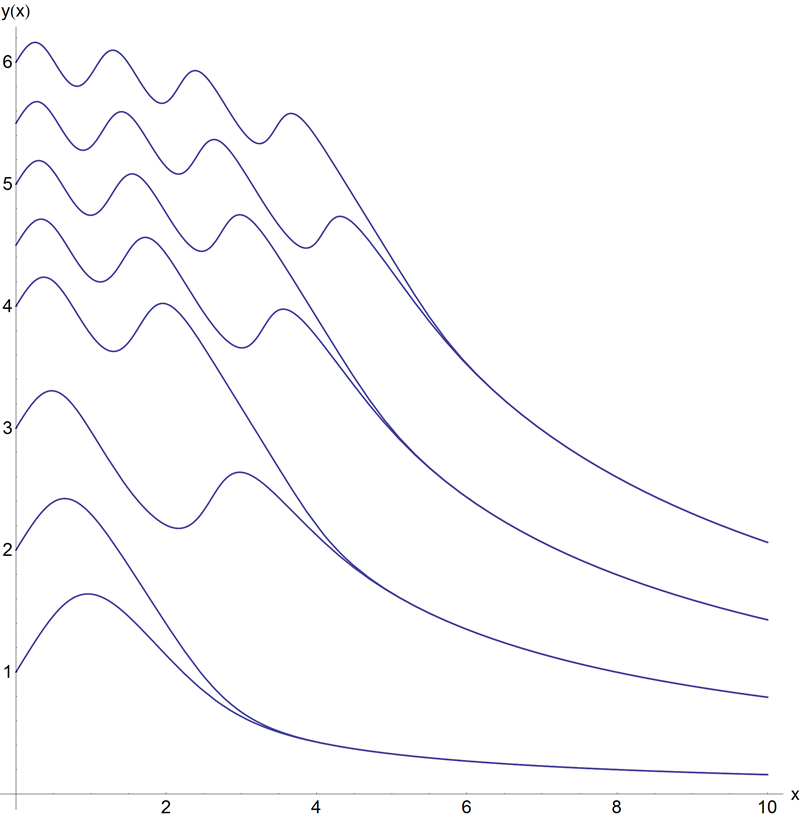
Figure 5: Solutions to the differential equation $y^{\prime}(x)=\cos(xy)$ for various initial conditions. Note that the solutions bunch together into discrete strands as $x$ increases.

We cannot solve (45) exactly, but we can use asymptotics to determine the features of the solutions in Fig. 5. To do so, we must first examine the behavior of the quantized strands for large $x$. Note that each strand becomes horizontal as $x\to\infty$ and that the solutions to the differential equation have zero slope on the hyperbolas

$$xy=\left(n+\textstyle{\frac{1}{2}}\right)\pi,$$ (46)

where $n$ is an integer (see Fig. 6). This suggests that the possible leading asymptotic behavior of $y(x)$ for large $x$ is given by

$$y(x)\sim\frac{\left(n+\textstyle{\frac{1}{2}}\right)\pi}{x}\quad(x\to\infty).$$ (47)

To verify (47) one must determine the higher-order corrections to this asymptotic behavior. These corrections take the form of a series in inverse powers of $x$:

$$y(x) \sim \frac{\left(n+\textstyle{\frac{1}{2}}\right)\pi}{x}\left[1+(-1)^{n}\frac{1}{x^{2}}+\frac{3}{x^{4}}+(-1)^{n}\frac{90+\left(n+\textstyle{\frac{1}{2}}\right)^{2}\pi^{2}}{6x^{6}}+\frac{315+8\left(n+\textstyle{\frac{1}{2}}\right)^{2}\pi^{2}}{3x^{8}}\right.$$ (48)

$$\qquad\left.+(-1)^{n}\frac{37800+1440\left(n+\textstyle{\frac{1}{2}}\right)^{2}\pi^{2}+3\left(n+\textstyle{\frac{1}{2}}\right)^{4}\pi^{4}}{40x^{10}}+\ldots\right]\quad(x\to\infty).$$

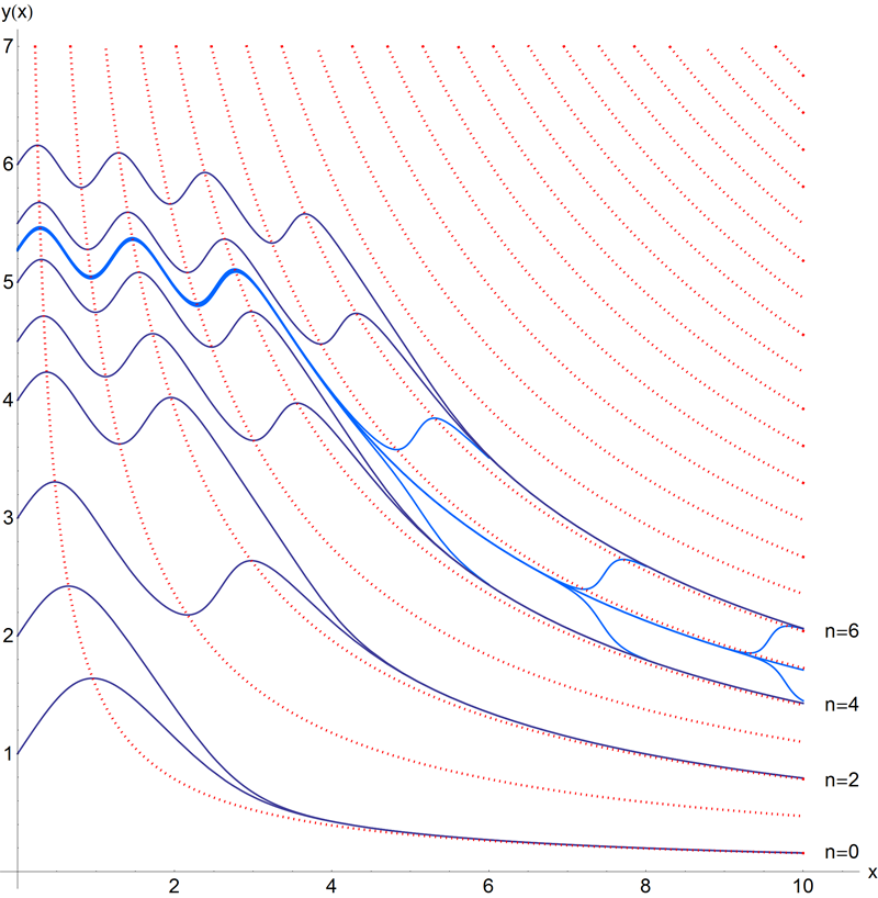
Figure 6: Solutions (solid lines) to $y^{\prime}(x)=\cos(xy)$ for various initial conditions. The slope of $y(x)$ vanishes on the hyperbolas (dotted lines) $xy=\left(n+\textstyle{\frac{1}{2}}\right)\pi$, where $n=0,\,1,\,2,\,\ldots$. Asymptotic analysis beyond all orders explains why solutions bunch together and approach the even-numbered hyperbolas. When $n$ is odd, the curves near the hyperbolas are unstable and veer away from the hyperbolas. To illustrate this instability, three initial conditions on either side of the separatrix initial condition $y(0)=5.276\,032\,283\,736\,901\,518\,295\,442\ldots$ are shown. The solutions beginning at $y(0)=5.287$ and at $y(0)=5.266$ veer off between $x=4$ and $x=5$, those beginning at $y(0)=5.276\,032\,296$ and at $y(0)=5.276\,032\,267$ veer off near $x=7$, and those beginning at $y(0)=5.276\,032\,283\,736\,901\,784$ and at $y(0)=5.276\,032\,283\,736\,901\,484$ veer off near $x=9$.

A remarkable feature of the asymptotic behavior in (48) is that there is no arbitrary constant. In general, the exact solution to an ordinary differential equation of order $N$ must contain $N$ arbitrary constants of integration and the asymptotic behavior of the solution must also have $N$ arbitrary constants. (The constant $n$ is not arbitrary because it is required to take on integer values.) Thus, the paradox is that the complete asymptotic description of the solution to (45) must contain an arbitrary constant, and yet no such constant appears to any order in the asymptotic series in (48).

The resolution of this puzzle is that there is an arbitrary constant of integration in the asymptotic behavior (48), but it cannot be seen at the level of Poincaré asymptotics. In Poincaré asymptotics one ignores transcendentally small (exponentially small) contributions to the asymptotic behavior because such contributions are subdominant (negligible compared with every term in the asymptotic series). The missing constant of integration in (48) can only be found at the level of hyperasymptotics (asymptotics beyond all orders) FF7 ; FF8 ; FF9 .

To find the missing constant of integration, we first observe that the difference of two solutions to (45) that belong to different bunches (that is, corresponding to different values of $n$) approaches zero like $1/x$ for large $x$:

$$y_{m}(x)-y_{n}(x)\sim\frac{(m-n)\pi}{x}\quad(x\to\infty).$$ (49)

However, the difference between two solutions belonging to the same bunch is exponentially small. To see this, let $y(x)$ and $u(x)$ be two solutions in the $n$th bunch and let $D(x)=y(x)-u(x)$ be their difference. Then $D(x)$ obeys the differential equation

$$\frac{dD}{dx} = \cos(xy)-\cos(xu)$$ (50)

$$= -2\sin\left[\textstyle{\frac{1}{2}}xD(x)\right]\sin\left[\textstyle{\frac{1}{2}}x(y+u)\right]$$

$$\sim -xD(x)\sin\left[\left(n+\textstyle{\frac{1}{2}}\right)\pi+(-1)^{n}\left(n+\textstyle{\frac{1}{2}}\right)\pi/x^{2}+\ldots\right]\quad(x\to\infty)$$

$$\sim -xD(x)(-1)^{n}\cos\left[\left(n+\textstyle{\frac{1}{2}}\right)\pi/x^{2}+\ldots\right]\quad(x\to\infty)$$

$$\sim -xD(x)(-1)^{n}\left[1-\textstyle{\frac{1}{2}}\left(n+\textstyle{\frac{1}{2}}\right)^{2}\pi^{2}/x^{4}+\ldots\right]\quad(x\to\infty),$$

where we have assumed that $D(x)$ is exponentially small and hence that the average of $y(x)$ and $u(x)$ is given by (48). Thus, the solution for $D(x)$ is

$$D(x)\sim Ce^{-(-1)^{n}x^{2}/2}\left[1-(-1)^{n}\frac{\left(n+\textstyle{\frac{1}{2}}\right)^{2}\pi^{2}}{4x^{2}}+\ldots\right]\quad(x\to\infty),$$ (51)

where $C$ is an arbitrary multiplicative constant of integration because the differential equation (50) is linear.

The derivation of (51) is valid only when $n$ is an even integer because the function $D(x)$ is exponentially small only when $n$ is even. When $n$ is odd, the result in (51) is of course not valid; however, we learn from this asymptotic analysis that the asymptotic solutions in (48) are unstable for odd $n$. That is, nearby solutions veer off as $x$ increases and become part of the adjacent bunches of solutions (see Fig. 6). One solution, called a separatrix, lies at the boundary between solutions that veer upward and solutions that veer downward; the separatrices are the solutions whose asymptotic behaviors are given by (47) and (48) for odd $n$. On Fig. 6 the separatrix corresponding to $n=5$ is shown; this separatrix evolves from the initial condition $y(0)=5.276\,032\,283\,736\,901\,518\,295\,442\ldots$.

IV.2 Stokes’ wedges and complex probability contours

The complex probability density $\rho(z)$ for the quantum harmonic oscillator is the square of the eigenfunctions of the time-independent Schrödinger equation. These eigenfunctions vanish like $e^{-z^{2}/2}$ as $z\to\pm\infty$ on the real axis. More generally, these eigenfunctions vanish exponentially in two Stokes’ wedges of angular opening $\pi/2$ centered on the positive-real and the negative-real axes. We refer to these Stokes’ wedges as the good Stokes’ wedges because this is where the probability integral (22) converges. Conversely, the eigenfunctions grow exponentially as $|z|\to\infty$ in two bad Stokes’ wedges of angular opening $\pi/2$ centered on the positive-imaginary and negative-imaginary axes. The probability integral clearly diverges if the integration contour terminates in a bad wedge.

Our objective is to find a path in the complex-$z$ plane on which the probability is real and positive. This path then serves as the integration contour for the integral in (22). The total probability can only be normalized to unity if this integral converges. Therefore, this contour of integration must originate inside one good Stokes’ wedge and terminate inside the other good Stokes’ wedge.

When we began working on this problem, we were surprised and dismayed to find that, apart from the trivial contour lying along the real axis, a continuous path originating and terminating in the good Stokes’ wedges simply does not exist! The (wrong) conclusion that one might draw from the nonexistence of a continuous integration path is that it is impossible to extend the quantum-mechanical harmonic oscillator (and quantum mechanics in general) into the complex domain without losing the possibility of having a local probability density.

To investigate the provenance of these difficulties it is necessary to perform an asymptotic analysis of the differential equation (44) that defines the integration contour. Using the techniques explained in the previous subsection, we find that deep inside the Stokes’ wedges, the solutions to this differential equation approach the centers of the wedges. Specifically, in the good Stokes’ wedge

$$y(x)\sim\frac{n\pi}{2x}\quad(x\to+\infty),$$ (52)

where $n$ is an integer, while inside the bad Stokes’ wedge

$$x(y)\sim\frac{(m+\textstyle{\frac{1}{2}})\pi}{2y}\quad(y\to+\infty),$$ (53)

where $m$ is an integer. Thus, as $|z|\to\infty$, the integration paths become quantized in the same manner as solutions to the toy-model discussed above. However, solutions deep in the good wedges are all unstable (like the odd-$n$ solutions in the toy model), while solutions deep in the bad wedges are all stable (like the even-$n$ solutions in the toy model). Thus, as $|z|\to\infty$ in a bad wedge, all solutions combine into quantized bunches and then approach the curves in (53). On the other hand, as $|z|\to\infty$ in a good wedge, all solutions except for the isolated separatrices in (52) peel off, turn around, and leave the Stokes’ wedge. These solutions then approach infinity in one of the bad Stokes’ wedges. This behavior is illustrated in Fig. 7.

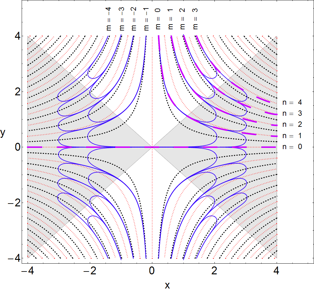
Figure 7: Numerical solutions (solid curves) to the differential equation (44) in the complex-$z=x+iy$ plane. These solutions have vanishing slope on the lightly dotted hyperbolas and infinite slope on the heavily dotted hyperbolas. There are two “good” Stokes’ wedges (dark shading) inside of which $\rho(z)$ decays to 0 exponentially as $|z|\to\infty$ along the solution curves and there are two “bad” Stokes’ wedges (unshaded) inside of which $\rho(z)$ grows exponentially as $|z|\to\infty$ along the solution curves. Note that as a typical solution curve goes more deeply into a good Stokes’ wedge, the curve becomes unstable and eventually turns around. The solution curve then leaves the good Stokes’ wedge and is pulled around into a bad Stokes’ wedge. In the bad Stokes’ wedge curves are stable and continue on to $\pm i\infty$. The only curves that ever reach $\pm\infty$ in the good Stokes’ wedges are separatrices. Five such separatrix paths labeled $n=0$, $n=1$, $\ldots$, $n=4$ are shown as heavy dashed curves. One special separatrix path runs along the real axis and connects the good Stokes’ wedge at $-\infty$ to the good Stokes’ wedge at $+\infty$. This is the only continuous unbroken curve that connects the two good Stokes’ wedges. Eight bunches of curves (labeled by $m$) that enter the bad Stokes’ wedges are shown.

Because of the inherent instability in the differential equation (44), only a discrete set of separatrix solutions actually enter and remain inside the good Stokes’ wedges. Finding these special curves is the analog of calculating the eigenvalues of a time-independent Schrödinger equation. It is only possible to satisfy the boundary conditions on the eigenfunctions of a Schrödinger equation for a discrete set of eigenvalues. Thus, by analogy we could refer to these special separatrix paths in the complex plane as eigenpaths AAA . With the single exception of the path that runs along the real axis, all eigenpaths terminating in a good Stokes’ wedge must originate in a bad Stokes’ wedge, as shown in Fig. 7.

Thus, it appears that apart from the real axis there is no path along which the probability integral (22) converges. Despite this apparently insurmountable problem, it is actually possible to find contours in the complex-$z$ plane on which the probability density satisfies the three requirements (20) – (22), as we explain in the next subsection.

IV.3 Resolution of the problem posed in Subsection IV.2

Amazingly, it is possible to overcome the difficulties described in Subsec. IV.2. In this subsection we use asymptotic analysis beyond all orders to show that if the probability integral (22) is taken on a contour $C_{1}$ that enters a bad Stokes’ wedge and continues off to $\infty$ in the wedge and then the integration path emerges from the bad wedge along a different contour $C_{2}$, the combined integral along $C_{1}+C_{2}$ exists if $C_{1}$ and $C_{2}$ are solutions to (44). This conclusion is valid even though the integrals along $C_{1}$ and along $C_{2}$ are separately very strongly (exponentially!) divergent. This is the principal result of this paper.

Recall that on every contour that solves the differential equation (44), the infinitesimal probability $\rho(z)\,dz$ is real. Now the objective is to select from all these contours those special contours on which the integral (22) exists. For the ground state of the harmonic oscillator this integral becomes

$$I=\int dy\,e^{y^{2}}e^{-[x(y)]^{2}}\frac{1}{\sin[2yx(y)]}.$$ (54)

To analyze the integral (54) we must use the Poincaré asymptotic series expansion of $x(y)$ for large $y$,

$$x(y)\sim\frac{\left(m+\textstyle{\frac{1}{2}}\right)\pi}{2y}\left(1+\frac{1}{2y^{2}}+\frac{3}{4y^{4}}+\frac{45-\left(m+\textstyle{\frac{1}{2}}\right)^{2}\pi^{2}}{24y^{6}}+\ldots\right)\quad(y\to+\infty),$$ (55)

whose leading asymptotic behavior is given in (53). The coefficients in this asymptotic series are easily derived from the differential equation (44). The asymptotic behavior of $x(y)$ beyond all orders is also required. To find this behavior, we let $u(y)$ and $v(y)$ be two solutions to $\frac{dx}{dy}=\cos(2xy)/\sin(2xy)$ having the same value of $n$ (that is, belonging to the same bunch). The Poincaré asymptotic behavior of these solutions is given in (55), but if we define $D(y)\equiv u(y)-v(y)$, we find that

$$D(y)\sim Ce^{-y^{2}}\left[1+\frac{\left(m+\textstyle{\frac{1}{2}}\right)^{2}\pi^{2}}{4y^{2}}+\frac{12\left(m+\textstyle{\frac{1}{2}}\right)^{2}\pi^{2}+\left(m+\textstyle{\frac{1}{2}}\right)^{4}\pi^{4}}{32y^{4}}+\ldots\right]\quad(y\to+\infty),$$ (56)

where $C$ is an arbitrary constant.

Consider an integration contour that enters the bad Stokes’ wedge centered on the positive imaginary axis. This contour starts at $y=Y$, follows the path $x=u(y)$, and runs up to $y=+\infty$. The contour then leaves the wedge along the path $v(y)$, and it returns to $y=Y$. Such a contour is shown in Fig. 8. The total contribution along both paths $u(y)$ and $v(y)$ to this integral is

$$I = \int_{Y}^{\infty}dy\,e^{y^{2}}\left(\frac{e^{-[u(y)]^{2}}}{\sin[2yu(y)]}-\frac{e^{-[v(y)]^{2}}}{\sin[2yv(y)]}\right)$$ (57)

$$= \int_{Y}^{\infty}dy\,e^{y^{2}}\frac{\sin[2yv(y)]e^{-[u(y)]^{2}}-\sin[2yu(y)]e^{-[v(y)]^{2}}}{\sin[2yu(y)]\sin[2yv(y)]}.$$

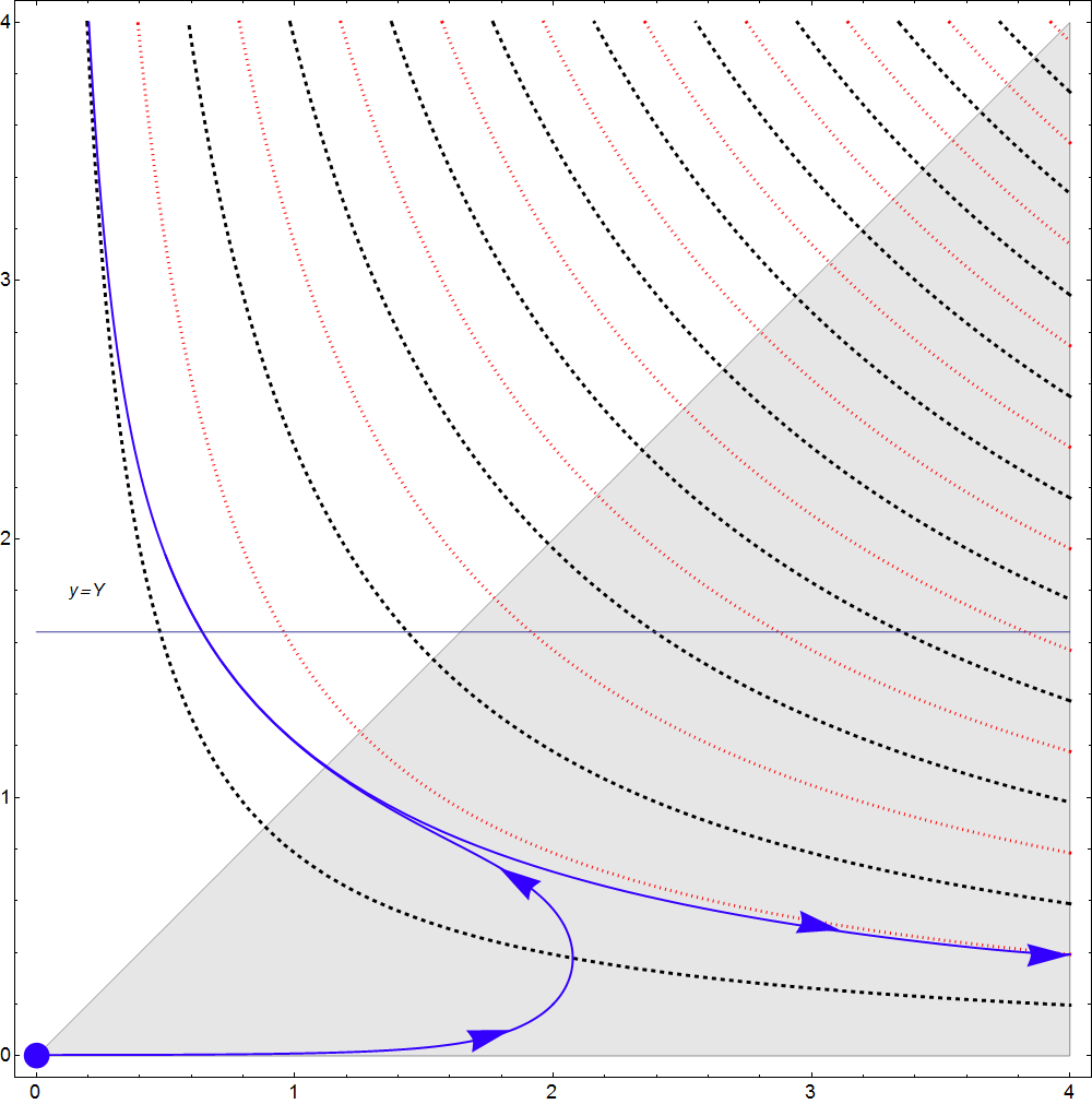
Figure 8: A contour in the complex-$z$ plane comprised of two numerical solutions to (44). The first path starts on the positive-imaginary axis at $y=0.003\,324\,973\,872\,707\,912$ (the starting point is indicated by a dot), and after it becomes vertical, it veers off to $y=\infty$ in the bad Stokes’ wedge. The second path is the separatrix belonging to the same bunch as the first path. This separatrix leaves the bad Stokes’ wedge and runs to $x=\infty$ in the good Stokes’ wedge. Even though the probability density blows up exponentially in the bad Stokes’ wedge, it is shown in (65) that the integral of the probability density from the value $y=Y$ up to $y=\infty$ along the first path and then from $y=\infty$ down to $y=Y$ along the second (separatrix) path is convergent.

Let us now investigate the convergence of this integral. We approximate the denominator of the integrand by using ordinary Poincaré asymptotics in which we ignore the transcendentally small difference between $u(y)$ and $v(y)$. We first establish that

$$2yu(y)\sim 2yv(y) \sim \sin\left[\left(m+\textstyle{\frac{1}{2}}\right)\pi+\frac{\left(m+\textstyle{\frac{1}{2}}\right)\pi}{2y^{2}}+\frac{3\left(m+\textstyle{\frac{1}{2}}\right)\pi}{4y^{4}}+\ldots\right]$$ (58)

$$\sim (-1)^{m}\cos\left[\frac{\left(m+\textstyle{\frac{1}{2}}\right)\pi}{2y^{2}}+\frac{3\left(m+\textstyle{\frac{1}{2}}\right)\pi}{4y^{4}}+\ldots\right]$$

$$\sim (-1)^{m}\left[1-\frac{\left(m+\textstyle{\frac{1}{2}}\right)^{2}\pi^{2}}{8y^{4}}+\ldots\right]\quad(y\to+\infty).$$

Thus, the denominator is given approximately by

$$\sin[2yu(y)]\sin[2yv(y)]\sim 1-\frac{\left(m+\textstyle{\frac{1}{2}}\right)^{2}\pi^{2}}{4y^{4}}+{\rm O}\left(\frac{1}{y^{6}}\right)\quad(y\to+\infty).$$ (59)

Next, we approximate the numerator of (57). Since $u(y)$ and $v(y)$ are small as $y\to+\infty$, we expand the exponentials. Keeping two terms in the expansion, we find that

$$\sin[2yv(y)]e^{-[u(y)]^{2}}-\sin[2yu(y)]e^{-[v(y)]^{2}}$$

$$\qquad\sim\sin[2yv(y)]\left(1-[u(y)]^{2}+\ldots\right)-\sin[2yu(y)]\left(1-[v(y)]^{2}+\ldots\right)$$ (60)

as $y\to+\infty$. Let us see what happens if we neglect the terms of order $u^{2}$ and $v^{2}$ and keep only the first pair of terms in (60). Using the trigonometric identity

$$\sin\alpha-\sin\beta=2\cos\left(\frac{\alpha+\beta}{2}\right)\sin\left(\frac{\alpha-\beta}{2}\right),$$ (61)

we find that the numerator has the following hyperasymptotic form:

$$\sin[2yv(y)]-\sin[2yu(y)] \sim 2\cos\left[\left(m+\textstyle{\frac{1}{2}}\right)\pi+\frac{\left(m+\textstyle{\frac{1}{2}}\right)\pi}{2y^{2}}+\frac{3\left(m+\textstyle{\frac{1}{2}}\right)\pi}{4y^{4}}\right]\sin(-yD)$$ (62)

$$\sim 2yD(y)(-1)^{m}\sin\left[\frac{\left(m+\textstyle{\frac{1}{2}}\right)\pi}{2y^{2}}+\frac{3\left(m+\textstyle{\frac{1}{2}}\right)\pi}{4y^{4}}\right]$$

$$\sim (-1)^{m}\frac{D(y)}{y}\left[\left(m+\textstyle{\frac{1}{2}}\right)\pi+\frac{3\left(m+\textstyle{\frac{1}{2}}\right)\pi}{2y^{2}}+{\rm O}\left(\frac{1}{y^{4}}\right)\right].$$

Hence, the leading-order contribution to the integrand of the integral in (57) gives

$$\int_{Y}^{\infty}dy\,e^{y^{2}}(-1)^{m}\frac{D(y)}{y}\left(m+\textstyle{\frac{1}{2}}\right)\pi.$$ (63)

Thus, apart from an overall multiplicative constant, this integral has the form $\int_{Y}^{\infty}dy/y$. This integral is not exponentially divergent, but it is still logarithmically divergent and thus it is not acceptable.

Fortunately, this logarithmic divergence cancels if we include higher-order terms in (60) in the calculation; including the quadratic terms in the expansion of the exponentials is sufficient to make the integral (57) converge. In addition to the terms that we examined in (62), we also consider

$$[v(y)]^{2}\sin[2yu(y)]-[u(y)]^{2}\sin[2yv(y)]$$

$$\qquad=\left([v(y)]^{2}-[u(y)]^{2}\right)\sin[2yu(y)]+[u(y)]^{2}\left(\sin[2yu(y)]-\sin[2yv(y)]\right)$$

$$\qquad\sim-\pi(-1)^{m}\left(m+\textstyle{\frac{1}{2}}\right)D(y)\left[\frac{1}{y}+\frac{1}{2y^{3}}+{\rm O}\left(\frac{1}{y^{5}}\right)\right]$$

$$\qquad\qquad+(-1)^{m}\left(m+\textstyle{\frac{1}{2}}\right)^{3}\pi^{3}D(y)\left[\frac{1}{4y^{3}}+{\rm O}\left(\frac{1}{y^{5}}\right)\right]\quad(y\to+\infty).$$ (64)

We combine this asymptotic contribution to the numerator of the integrand of (57) with the leading-order contribution in (62) and obtain a further cancellation. The resulting integral

$$\int_{Y}^{\infty}dy\,(-1)^{m}e^{y^{2}}D(y)\frac{\left(m+\textstyle{\frac{1}{2}}\right)\pi}{y^{3}}=C(-1)^{m}\left(m+\textstyle{\frac{1}{2}}\right)\int_{Y}^{\infty}\frac{dy}{y^{3}}$$ (65)

converges! Because this integral is convergent, a contour can begin at a point on the positive imaginary axis, run into and back out of the bad Stokes’ wedge at $y=+\infty$, and then terminate in the good Stokes’ wedge at $x=+\infty$. Such a contour, which begins at $y=0.003\,324\,973\,872\,707\,912$ on the imaginary axis, is shown in Fig. 9.

Finally, if we reflect this contour about the $y$ axis, we get a complete path originating in the left good Stokes’ wedge at $x=-\infty$, crossing the $y$ axis horizontally, and eventually terminating in the right good Stokes’ wedge at $x=+\infty$. Such a contour is shown in the upper plot in Fig. 9. Note that a contour that leaves the bad Stokes’ wedge need not leave on a separatrix path that terminates in the good Stokes’ wedge; instead, it can leave the bad Stokes’ wedge and follow a path that turns around and returns to the bad Stokes’ wedge. Such a path, which is shown in the lower plot in Fig. 9, finally leaves the bad Stokes’ wedge on a separatrix path and terminates in the good Stokes’ wedge. Thus, the contour can be multiply thatched before it eventually terminates in the good Stokes’ wedge.

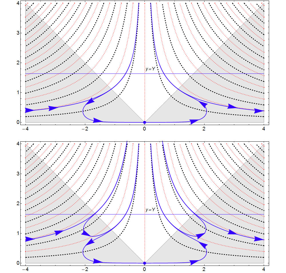
Figure 9: Complex contours that run from one good Stokes’ wedge to the other. In the upper plot a contour begins at $x=-\infty$ in the left good Stokes’ wedge (shaded region), leaves the good Stokes’ wedge along a separatrix path, and runs up to $i\infty$ in the bad Stokes’ wedge (unshaded region). The contour then continues downward along a path in the same bunch, crosses the imaginary axis at $y=0.003\,324\,973\,872\,707\,912$, and heads upwards into the same bad Stokes’ wedge. Finally, the contour re-emerges from the bad Stokes’ wedge and continues towards $x=+\infty$ along a separatrix path in the right good Stokes’ wedge. Contours have zero slope on the lightly dotted lines and infinite slope on the heavily dotted lines. In the lower plot the contour connecting the two good Stokes’ wedges visits the bad Stokes’ wedge four times instead of twice.

We remark that the device described here, in which the contour enters and then leaves a bad Stokes’ wedge, does not work with the method of steepest descents, which is a standard technique used to find the asymptotic behavior of integrals. When a steepest path runs off to $\infty$, it can only do so in a good Stokes’ wedge and not in a bad Stokes’ wedge; otherwise, the integral would diverge. In contrast, for the problem discussed in this paper the path of real probability has no choice; it necessarily enters the bad Stokes’ wedge, and it is the stable bunching of contours into quantized strands that saves the day.

IV.4 Safely crossing lightly dotted lines and heavily dotted lines

There is one more potential problem that must be considered before we can claim to have a complete contour on which the probability density is positive and normalizable. It is necessary to show that the sign of the probability density does not change if the contour crosses one of the hyperbolas $2xy=n\pi$ on which $y^{\prime}(x)=0$, or $2xy=\left(m+\textstyle{\frac{1}{2}}\right)\pi$, on which $y^{\prime}(x)=\infty$. These hyperbolas are shown as lightly dotted and heavily dotted lines in Fig. 9.

We can see that the contours in Fig. 9 cross both lightly and heavily dotted lines. When this happens, the sign of the denominators in (31) or (32) change, so at first one might think that the probability density along the contour would not remain positive. To address this concern, we rewrite each of the differential probabilities (31) and (32) as a differential probability proportional to the infinitesimal path length element $ds$ by using the standard formula $ds=\sqrt{dx^{2}+dy^{2}}$. Thus, in (31), for example, we eliminate $dx$ in favor of $ds$ and obtain

$$dx=\frac{ds}{\sqrt{1+\left(\frac{dy}{dx}\right)^{2}}}.$$ (66)

We then substitute the differential equation (29) into (66) and get

$${\rm Re}(\rho dz)=e^{-x^{2}+y^{2}}\sqrt{[S(x,y)]^{2}+[T(x,y)]^{2}}ds.$$ (67)

Clearly, this form of the infinitesimal probability contribution along the contour is explicitly positive and cannot change sign.

Where is the error in the reasoning that led us to worry that the sign of ${\rm Re}(\rho dz)$ might change? We note that the contour in Fig. 9 crosses a heavily dotted line near $x=2$ and $y=1/2$. Thus, the denominator of (31) does indeed change sign. However, as the probability curve becomes vertical, it simultaneously changes direction (that is, it runs backward). This is equivalent to $dx$ changing sign, and this change in sign compensates for the change in sign of the denominator. Thus, all along the contour the infinitesimal contributions to the total probability remain positive.

V Complex Probability Density for Higher-Energy States of the Harmonic Oscillator

In this section we generalize the analysis of Sec. IV to the excited states of the quantum harmonic oscillator. The eigenfunctions of these states differ from the ground state in that they have nodes on the real axis. As a consequence, the functions $S(x,y)$ and $T(x,y)$ in (26) become more complicated and as a result the differential equation (29), which determines the probability eigenpaths, is correspondingly more challenging to analyze.

The first excited state $\psi_{1}(z)=ze^{-z^{2}/2}$, whose energy is 3, has a single node, which is located at the origin. For this eigenfunction $S(x,y)=x^{2}-y^{2}$ and $T(x,y)=2xy$. Thus, the differential equation (29) becomes

$$\frac{dy}{dx}=\frac{(x^{2}-y^{2})\sin(2xy)-2xy\cos(2xy)}{(x^{2}-y^{2})\cos(2xy)+2xy\sin(2xy)}.$$ (68)

It is necessary to determine the asymptotic behavior of solutions to this equation near the node at the origin in the $(x,y)$ plane. To do so we seek a leading asymptotic behavior of the form $y(x)\sim ax+\ldots$ as $x\to 0$. Substituting this behavior into (68) gives an algebraic equation for $a$:

$$a=\frac{2a}{a^{2}-1}.$$ (69)

The solutions to this equation are $a=0$ and $a=\pm\sqrt{3}$, which indicates that eigenpaths can enter or leave the node in one of six possible directions separated by $60^{\circ}$. (These paths are indicated on Fig. 10, except that the trivial path along the real axis has been omitted.) Apart from the behavior in the vicinity of the node, the eigenpaths shown in this figure are qualitatively similar to those shown in Figs. 7 and 9.

Figure 10 shows that there are many compound eigenpaths connecting the two good Stokes’ wedges in addition to the conventional path along the real axis. A typical eigenpath begins in the left good Stokes’ wedge and runs along a separatrix into one of the bad Stokes’ wedges centered on the positive- or negative-imaginary axes. The path then emerges from and returns to the bad Stokes’ wedge several times before crossing the imaginary axis. This path crosses the imaginary axis in two possible ways: (i) The path may cross the imaginary axis at the node, and if it does, the path may form a cusp. (ii) The path may cross the imaginary axis at a point other that is not a node, in which case it must be horizontal at the crossing point. The path then enters and emerges from a bad Stokes’ wedge several more times before running off along a separatrix to infinity in the right good Stokes’ wedge.

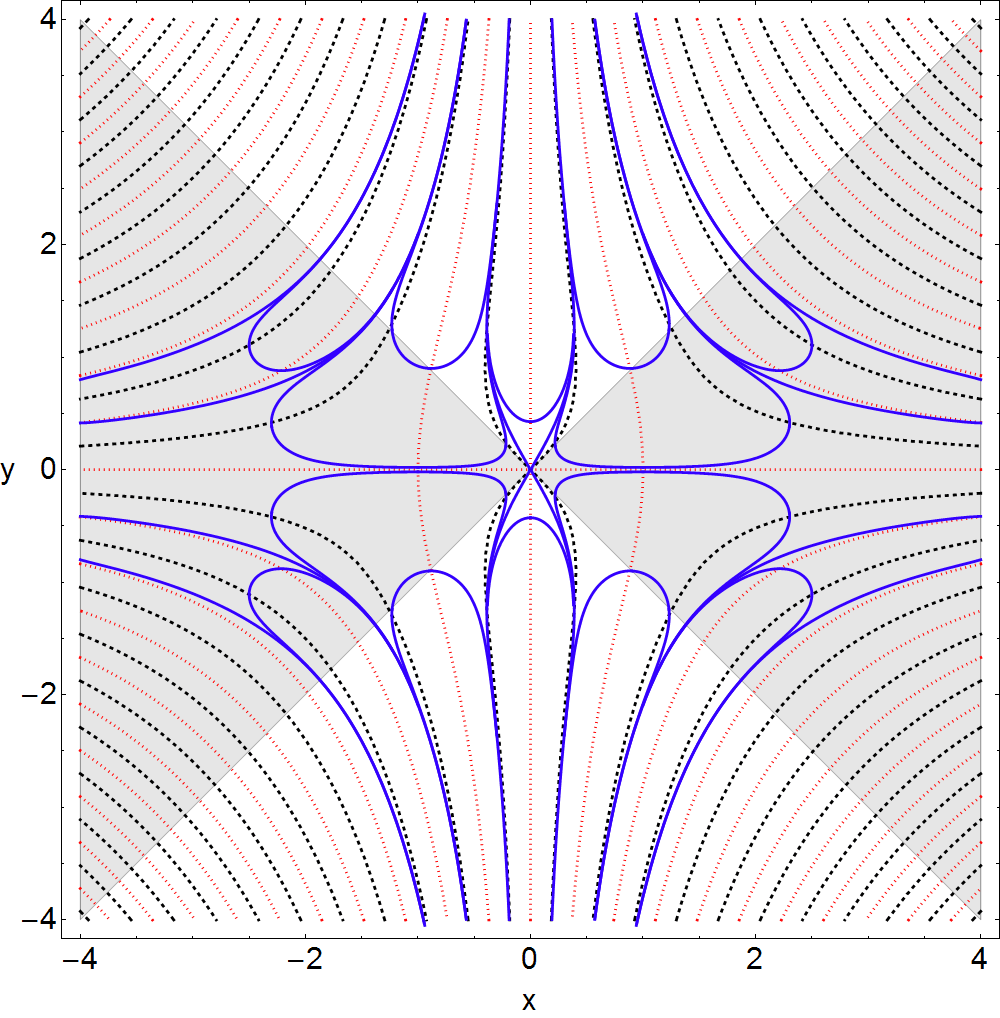
Figure 10: Complex contours that run from the left good Stokes’ wedge to the right good Stokes’ wedge for the first excited state of the quantum harmonic oscillator. Four contours (solid lines) that begin at $x=-\infty$ in the left good Stokes’ wedge (shaded region) are shown. These contours leave this Stokes’ wedge along separatrix paths and run off to $\pm i\infty$ in the upper and lower bad Stokes’ wedges (unshaded regions). After visiting a bad Stokes’ wedge one or more times, the contours pass through the node at the origin at $60^{\circ}$ angles to the horizontal. At this node the probability density vanishes. Then the contours repeat the process in the right-half plane and eventually enter the right good Stokes’ wedge along separatrix paths. Note that it is also possible to have a complex contour that does not pass through the node at the origin and still connects the good Stokes’ wedges. The solution curves are horizontal on the lightly dotted lines and vertical on the heavily dotted lines.

The eigenfunction representing the second excited state has the form $\psi_{2}(z)=(2z^{2}-1)e^{-z^{2}/2}$. The energy is 5. There are now two nodes, which are located on the real axis at $\pm 1/\sqrt{2}$. These nodes are shown on Fig. 11. The eigenpaths in Fig. 11 are qualitatively similar to those shown in Fig. 10. Like the eigenpaths shown in Fig. 10, the eigenpaths in Fig. 11 enter the nodes horizontally or at $\pm 60^{\circ}$ angles.

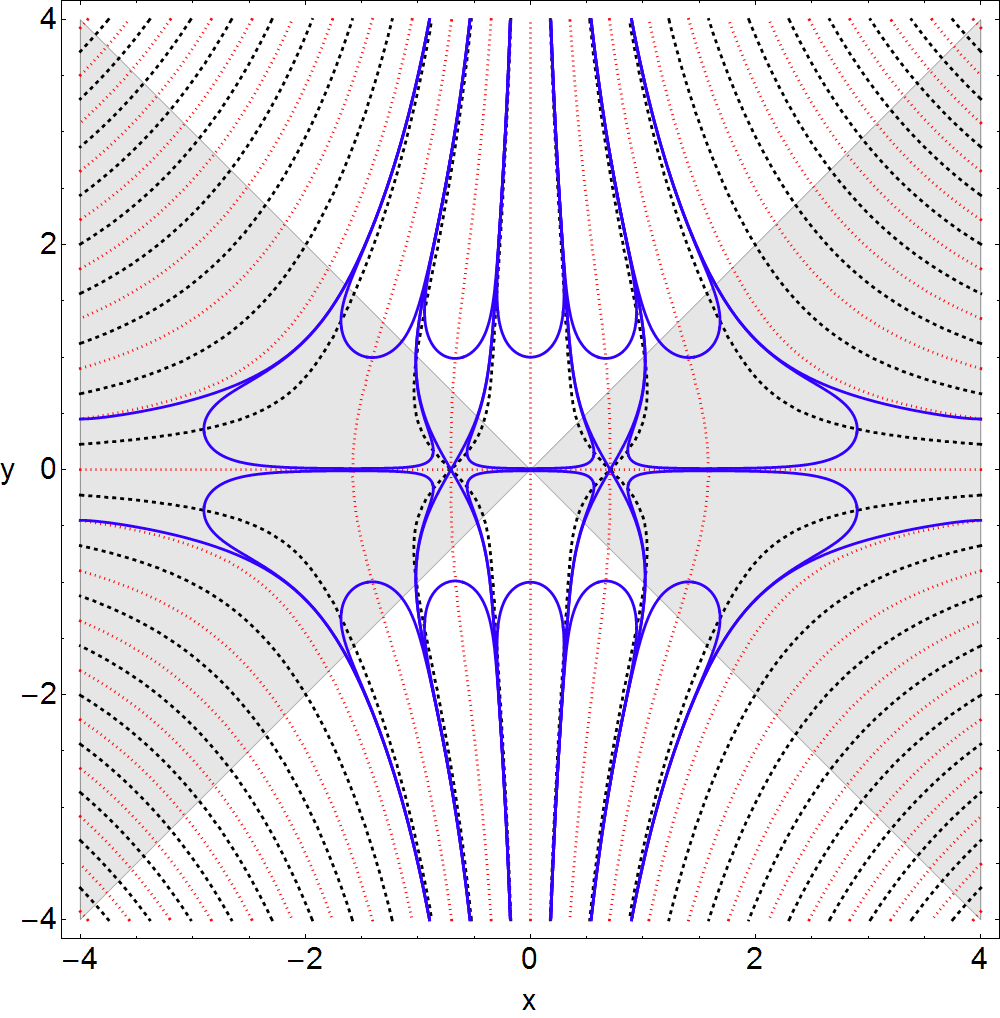
Figure 11: Complex contours that run from one good Stokes’ wedge to the other for the case of the second excited state of the quantum harmonic oscillator. Two contours (solid lines) that begin at $x=-\infty$ in the left good Stokes’ wedge (shaded region) are shown. These contours leave the left good Stokes’ wedge along separatrix paths and run off to $\pm i\infty$ in the upper and lower bad Stokes’ wedges (unshaded regions). After visiting the bad Stokes’ wedge one or more times, the contours pass through the left node on the real axis at $60^{\circ}$ angles to the horizontal. At this node the probability density vanishes. The contours then reenter the upper or lower bad Stokes’ wedges and pass through the right node on the real axis. After returning to the bad Stokes’ wedges yet again, the solution curves eventually enter the right good Stokes’ wedge along separatrix paths. The solution curves are horizontal on the lightly dotted lines and vertical on the heavily dotted lines.

VI Complex Probability Density for the Quasi-Exactly Solvable Anharmonic Oscillator

In this section we generalize the results of the previous two sections for the quantum harmonic oscillator to the more elaborate case of the quasi-exactly-solvable ${\cal P}{\cal T}$-symmetric anharmonic oscillator, whose Hamiltonian is given in (24). We consider here the special class of these Hamiltonians for which $b=0$ because the case $b\neq 0$ presents no additional features of interest. The time-independent Schrödinger equation for this Hamiltonian is

$$\left(-\frac{d^{2}}{dx^{2}}-x^{4}+2iax^{3}+a^{2}x^{2}-2iJx\right)\psi_{n}(x)=E_{n}\psi_{n}(x).$$ (70)

When $J$ is a positive integer, the first $J$ eigenfunctions have the form

$$\psi(x)=e^{-ix^{3}/3-ax^{2}/2}P_{J-1}(x),$$ (71)

where

$$P_{J-1}(x)=x^{J-1}+\sum_{k=0}^{J-2}c_{k}x^{k}$$ (72)

is a polynomial of degree $J-1$.

VI.1 Probability density in the complex plane for the ground state

We begin the analysis by considering the case $J=1$ for which the ground-state eigenfunction can be found exactly and in closed form:

$$\psi(x)=e^{-ix^{3}/3-ax^{2}/2}.$$ (73)

The associated ground-state energy is $E_{0}=a$. According to (18), the time-independent local probability density $\rho$ in the complex-$z$ plane for this eigenfunction is

$$\rho(z)=e^{-2iz^{3}/3-az^{2}}.$$ (74)

As in our study of the harmonic oscillator in Secs. IV and V, we take $z=x+iy$ and $dz=dx+idy$. We then obtain

$$\rho(z)dz=e^{2x^{2}y-2y^{3}/3-ax^{2}+ay^{2}}(\cos\theta-i\sin\theta)(dx+idy),$$ (75)

where

$$\theta=-2xy^{2}+2x^{3}/3+2axy.$$ (76)

Consequently, Condition I in (20), which requires that ${\rm Im}\,[\rho(z)dz]=0$, translates into the differential equation

$$\frac{dy}{dx}=\frac{\sin\theta}{\cos\theta}.$$ (77)

This differential equation is the analog of (44) for the harmonic oscillator. Also, Condition III in (22), which requires that the integral of ${\rm Re}\,[\rho(z)dz]$ exist, is the same as demanding that the following (equivalent) integrals exist:

$$\int{\rm Re}\,[dz\rho(z)] = \int(dx\cos\theta+dy\sin\theta)e^{2x^{2}y-2y^{3}/3-ax^{2}+ay^{2}}$$ (78)

$$= \int\frac{dy}{\sin\theta}e^{2x^{2}y-2y^{3}/3-ax^{2}+ay^{2}}$$

$$= \int\frac{dx}{\cos\theta}e^{2x^{2}y-2y^{3}/3-ax^{2}+ay^{2}}.$$ (79)

The integration contours for the integrals above must terminate in good Stokes’ wedges in order that the integrals converge. The locations and opening angles of the Stokes’ wedges are identified by determining where the probability density $\rho(z)$ is exponentially growing or decaying. There are six Stokes’ wedges, each having angular opening $\pi/3$. Of the three good Stokes’ wedges [where $\rho(z)$ decays exponentially] one is centered about the positive-imaginary axis and the other two lie adjacent to and below the positive-real and negative-real axes. One of the three bad Stokes’ wedges is centered about the negative-imaginary axis and the other two lie adjacent to and above the positive-real and negative-real axes. The good and bad Stokes’ wedges are shown in Fig. 12 as shaded and unshaded regions.

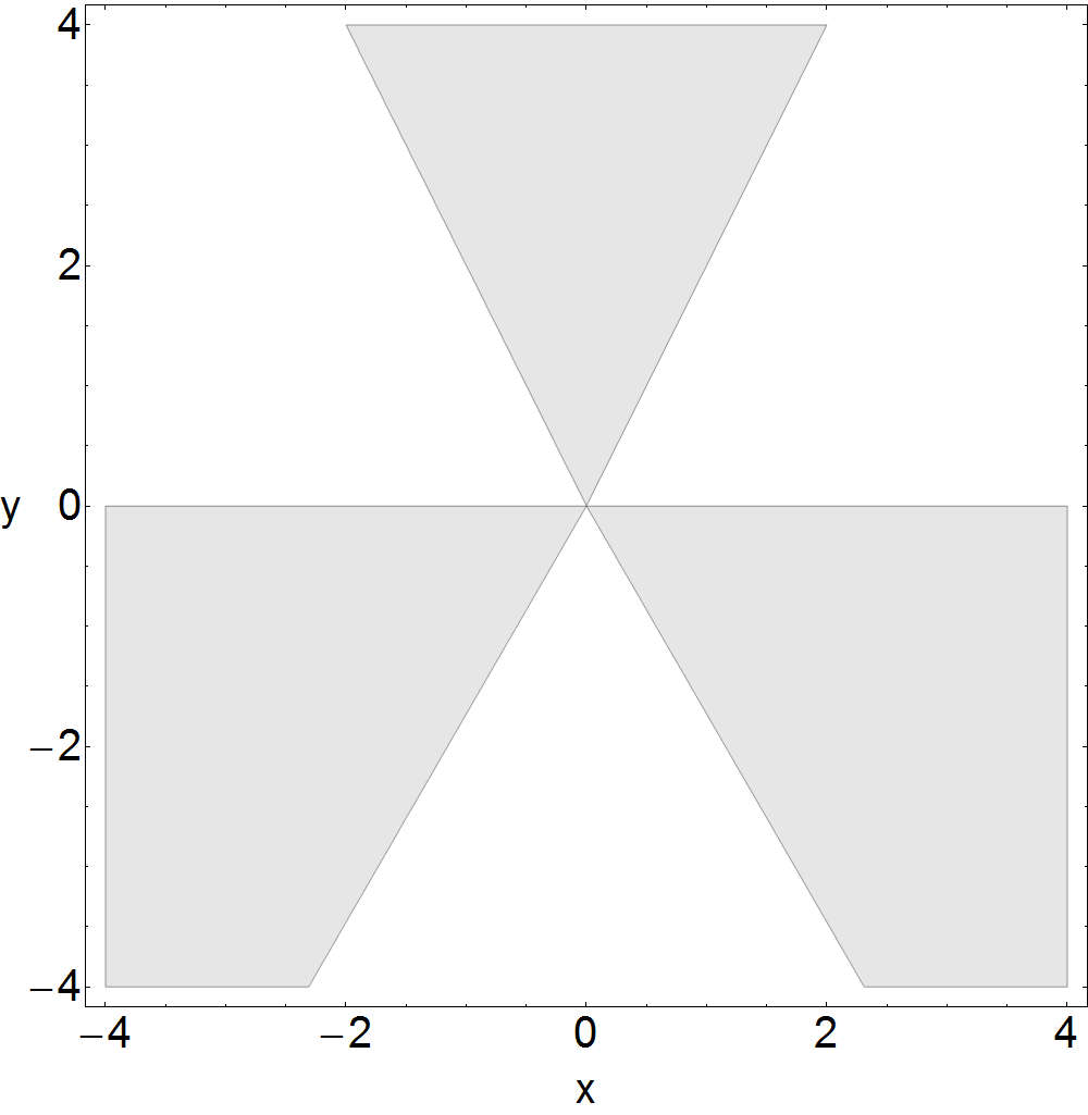
Figure 12: Good Stokes’ wedges (shaded regions) and bad Stokes’ wedges (unshaded regions) for the quasi-exactly-solvable ${\cal P}{\cal T}$ anharmonic oscillator in (70). In the three good Stokes’ wedges the eigenfunctions decay to zero like the exponential of a cubic [see (73)]. The eigenfunctions grow like the exponential of a cubic in the bad Stokes’ wedges.

1. Asymptotic analysis of solutions in the good Stokes’ wedge below the positive-real axis.

We begin by finding the asymptotic behavior of a function $y(x)$ that solves the differential equation (77) and which approaches the center of the good wedge that lies adjacent to and below the positive-real $z$ axis. (Because of ${\cal P}{\cal T}$ symmetry, which is simply left-right symmetry in the complex-$z$ plane, the left good wedge is treated in a similar fashion.) The center of this wedge lies at an angle of $-\pi/6$ in the complex-$z$ plane, so we seek a solution $y(x)$ that satisfies the asymptotic condition

$$y\sim-x/\sqrt{3}\quad(x\to+\infty).$$ (80)

The full asymptotic series approximation for such a solution has the form

$$y\sim-\frac{x}{\sqrt{3}}+A_{1}+\frac{A_{2}}{x}+\frac{A_{3}}{x^{2}}+\frac{A_{4}}{x^{3}}+\frac{A_{5}}{x^{4}}+\frac{A_{6}}{x^{5}}+\ldots\,.$$ (81)

To determine the coefficients in this series we observe that if we choose

$$A_{1}=\textstyle{\frac{1}{2}}a\quad{\rm and}\quad A_{2}=-\frac{1}{8}a^{2}\sqrt{3},$$ (82)

then $\theta\to 4A_{3}/\sqrt{3}$ as $x\to\infty$. Then, using the differential equation (77), we get $-1/\sqrt{3}=\tan(4A_{3}/\sqrt{3})$, which gives

$$A_{3}=\frac{\sqrt{3}}{4}\left(n-\frac{1}{6}\right)\pi.$$ (83)

With this choice of $A_{3}$, we can use the differential equation to determine all of the higher-order coefficients in the asymptotic expansion:

$$A_{4} = \frac{3\sqrt{3}a^{4}}{128},$$

$$A_{5} = \frac{9a^{2}-48a^{2}A_{3}}{128},$$

$$A_{6} = \frac{512\sqrt{3}A_{3}^{2}-384\sqrt{3}A_{3}-9a^{6}\sqrt{3}}{1024}.$$ (84)

Next, we perform an asymptotic analysis beyond all orders to determine whether the solutions whose asymptotic behavior is given in (81) are stable. Let

$$D(x)\equiv y_{1}(x)-y_{2}(x),$$ (85)

where $y_{1}$ and $y_{2}$ belong to the $n$th bunch of solutions. Then, $D(x)$ satisfies the differential equation

$$D^{\prime}(x)=\frac{\sin\theta_{1}}{\cos\theta_{1}}-\frac{\sin\theta_{2}}{\cos\theta_{2}}=\frac{\sin(\theta_{1}-\theta_{2})}{\cos\theta_{1}\cos\theta_{2}}.$$ (86)

If we now assume that $D(x)$ is small, we obtain the asymptotic approximation

$$\theta_{1}-\theta_{2}\sim(-4xy+2ax)D(x)\quad(x\to+\infty),$$ (87)

and since

$$\theta\sim\left(n-\frac{1}{6}\right)\pi+\frac{a^{2}}{32\sqrt{3}x^{2}}\quad(x\to+\infty),$$ (88)

we obtain the asymptotic approximation

$$\frac{1}{\cos^{2}\theta}\sim\frac{4}{3}-\frac{a^{2}}{4x^{2}}\quad(x\to+\infty).$$ (89)

Thus, $D(x)$ satisfies the approximate linear differential equation

$$D^{\prime}(x)\sim D(x)\left(\frac{16x^{2}}{3\sqrt{3}}+\frac{a^{2}}{\sqrt{3}}\right)\quad(x\to+\infty),$$ (90)

whose solution contains the arbitrary multiplicative constant $K$:

$$D(x)\sim Ke^{16\sqrt{3}x^{3}/27+a^{2}\sqrt{3}x/3}\quad(x\to+\infty).$$ (91)

Note that as $x\to\infty$, the difference function $D(x)$ grows exponentially with increasing $x$, which contradicts the assumption that $D(x)$ is small as $x\to+\infty$. We conclude that in the good wedge all solutions are unstable and that only a discrete set of isolated separatrix paths can continue deep into the good wedge without turning around and leaving the wedge. (For the case of the quantum harmonic oscillator the analogous unstable separatrix paths are shown in Fig. 7.)

Numerical analysis (for the case $a=1$) confirms that there exists just one unstable separatrix that runs directly from the left good Stokes’ wedge to the right good Stokes’ wedge. This path is displayed in Fig. 13. The path shown in this figure is the exact analog of the path in Fig. 7 that runs along the real axis from $-\infty$ to $\infty$ for the case of the quantum harmonic oscillator.

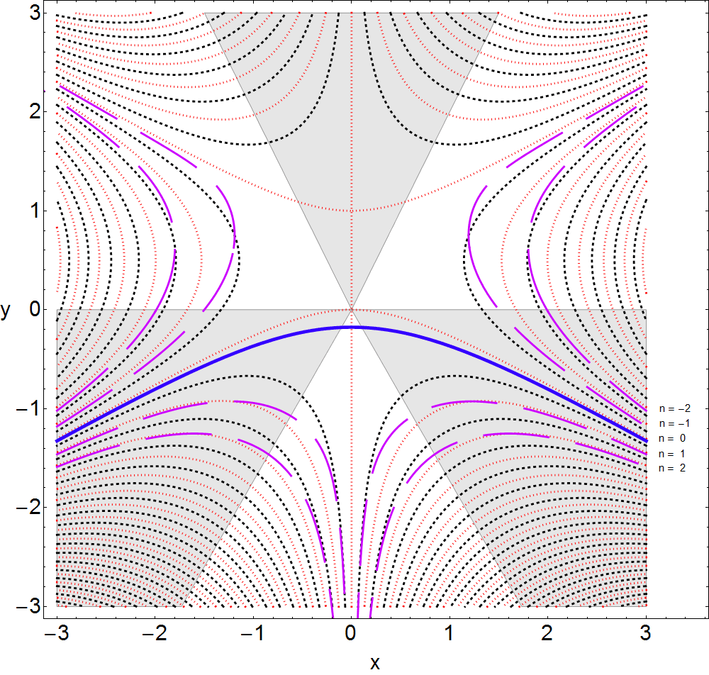
Figure 13: Separatrix paths for the ground state of the quasi-exactly-solvable ${\cal P}{\cal T}$ anharmonic oscillator whose Hamiltonian is given in (24). (We have chosen the value of the parameter $a$ to be $1$.) The asymptotic behavior of these paths in the right good Stokes’ wedge is given in (81). Exactly one separatrix path (heavy continuous line), which corresponds to the choice $n=0$ in (83), runs from the left good Stokes’ wedge directly to the right good Stokes’ wedge without veering into a bad Stokes’ wedge. This path, which is the analog of the path along the real axis for the quantum harmonic oscillator, crosses the imaginary axis at $y=-0.176\,651\,795\,619\,462\,368$. Other separatrix paths (heavy dashed lines) for the cases $n=\pm 1$ and $n=\pm 2$ are shown; these paths run from good Stokes’ wedges to bad Stokes’ wedges. The solutions to the differential equation are horizontal on the lightly dotted lines and vertical on the heavily dotted lines.

2. Asymptotic analysis of solutions in the bad Stokes’ wedge above the positive-real axis.

Next, we construct solutions to the differential equation (77) that approach the center of the bad wedge as $x\to\infty$. Since the center of the wedge lies at an angle of $\pi/6$ above the real axis, such solutions have the asymptotic form

$$y\sim\frac{x}{\sqrt{3}}+B_{1}+\frac{B_{2}}{x}+\frac{B_{3}}{x^{2}}+\frac{B_{4}}{x^{3}}+\frac{B_{5}}{x^{4}}+\frac{B_{6}}{x^{5}}\ldots\quad(x\to+\infty).$$ (92)

We determine $B_{1}$ and $B_{2}$ so that $\theta$ approaches a constant as $x\to+\infty$. We find that if

$$B_{1}=\textstyle{\frac{1}{2}}a\quad{\rm and}\quad B_{2}=\frac{1}{8}a^{2}\sqrt{3},$$ (93)

then $\theta\to-4B_{3}/\sqrt{3}$ as $x\to\infty$. Substituting into the differential equation we get $1/\sqrt{3}=\tan(-4B_{3}/\sqrt{3})$, which gives

$$B_{3}=\frac{\sqrt{3}}{4}\left(n-\frac{1}{6}\right)\pi.$$ (94)

The higher-order coefficients are

$$B_{4} = -\frac{3\sqrt{3}a^{4}}{128},$$

$$B_{5} = \frac{9a^{2}-48a^{2}B_{3}}{128},$$

$$B_{6} = \frac{-512\sqrt{3}B_{3}^{2}+384\sqrt{3}B_{3}+9a^{6}\sqrt{3}}{1024}.$$ (95)

We perform an asymptotic analysis beyond all orders to determine if such solutions are stable. To do so, we define $D(x)\equiv y_{1}(x)-y_{2}(x)$, where $y_{1}$ and $y_{2}$ belong to the $n$th bunch of solutions, and we find that

$$D(x)\sim Ke^{-16\sqrt{3}x^{3}/27-a^{2}\sqrt{3}x/3}\quad(x\to\infty),$$ (96)

where $K$ is an arbitrary constant. Since $D(x)$ vanishes exponentially for large $x$, the solutions in this bad wedge are all stable; that is, they bunch together as $x\to+\infty$. The result here is analogous to that in (56) for the harmonic oscillator.

Because these solutions are in a bad wedge, they blow up like the exponential of a cubic as they penetrate deeper into the wedge. Thus, the integral

$$\int_{z_{0}}^{\infty}{\rm Re}\,[dz\rho(z)]=\int_{z_{0}}^{\infty}\frac{dx}{\cos\theta}e^{2x^{2}y-2y^{3}/3-ax^{2}+ay^{2}}$$ (97)

diverges. Thus, the question is, Is it possible to have a contour that enters and leaves this wedge in such a way that this integral exists? That is, if $y_{1}(x)$ and $y_{2}(x)$ are two solutions that enter that bad Stokes’ wedge, does the integral

$$I=\int_{x=L}^{\infty}{\rm Re}\,[dz\rho(z)]=\int_{x=L}^{\infty}dx\,e^{-ax^{2}}\left(\frac{e^{2x^{2}y_{1}-2y_{1}^{3}/3+ay_{1}^{2}}}{\cos\theta_{1}}-\frac{e^{2x^{2}y_{2}-2y_{2}^{3}/3+ay_{2}^{2}}}{\cos\theta_{2}}\right)$$ (98)

converge? The answer to this question is no.

The problem here is that the cubic polynomial in the exponent,

$$2x^{2}y-\frac{2}{3}y^{3}+ay^{2}\sim\frac{16\sqrt{3}}{27}x^{3}+ax^{2}+{\rm O}(x)\quad(x\to\infty),$$ (99)

causes the integrand of the integral to blow up like the exponential of a cubic. Thus, we cannot use the argument used earlier for the harmonic oscillator, where we were able to expand the exponentials and to calculate the difference in terms of hyperasymptotics. Thus, even if the integration contour enters and leaves the wedge, the resulting integral will not converge. Hence, it is not possible to leave this bad wedge as we did for the bad wedge of the harmonic oscillator; a contour that enters this bad wedge is trapped forever.

3. Asymptotics of solutions in the bad Stokes’ wedge centered about the negative-imaginary axis.

This time we want to study the differential equation

$$\frac{dx}{dy}=\frac{\cos\theta}{\sin\theta}$$ (100)

and we want to investigate the integral in (78) for large negative $y$. This integral has the form

$$\int dy\,e^{-2y^{3}/3+ay^{2}}\frac{e^{2x^{2}y-ax^{2}}}{\sin\theta}.$$ (101)

A solution that approaches the center of the wedge has the form

$$x(y)\sim\frac{C_{1}}{y^{2}}+\frac{C_{2}}{y^{3}}+\frac{C_{3}}{y^{4}}+\frac{C_{4}}{y^{5}}+\frac{C_{5}}{y^{6}}+\frac{C_{6}}{y^{7}}+\ldots\,.$$ (102)

If we take

$$C_{2}=aC_{1}\quad{\rm and}\quad C_{3}=a^{2}C_{1},$$ (103)

then for large negative $y$ we get $\theta\sim-2C_{1}+{\rm O}\left(y^{-3}\right)$ and this balances $dx/dy={\rm O}\left(y^{-3}\right)$ if $\cos(-2C_{1})=0$, that is, if

$$C_{1}=-\textstyle{\frac{1}{2}}\left(n+\textstyle{\frac{1}{2}}\right)\pi.$$ (104)

We then get

$$C_{4} = (a^{3}-1)C_{1},$$

$$C_{5} = \textstyle{\frac{1}{2}}\left(2a^{4}-5a\right)C_{1},$$

$$C_{6} = \textstyle{\frac{1}{2}}\left(2a^{5}-9a^{2}\right)C_{1}.$$ (105)

Thus, as $y\to-\infty$, the asymptotic behavior of $x(y)$ is given by

$$x(y)\sim C_{1}\left(\frac{1}{y^{2}}+\frac{a}{y^{3}}+\frac{a^{2}}{y^{4}}+\frac{a^{3}-1}{y^{5}}+\frac{2a^{4}-5a}{2y^{6}}+\frac{2a^{5}-9a^{2}}{2y^{7}}+\ldots\right).$$ (106)

Now we test for stability: Let

$$D(y)\equiv x_{1}(y)-x_{2}(y)$$ (107)

be the difference of two solutions in the $n$th bunch. Then,

$$D^{\prime}(y)=\frac{\cos\theta_{1}}{\sin\theta_{1}}-\frac{\cos\theta_{2}}{\sin\theta_{2}}=\frac{\sin(\theta_{2}-\theta_{1})}{\sin\theta_{1}\sin\theta_{2}}.$$ (108)

But for large negative $y$,

$$\theta_{2}-\theta_{1}\sim 2D(y)(y^{2}-x^{2}-ay)\quad(y\to-\infty).$$ (109)

The denominator is just $[\sin\left(n+\textstyle{\frac{1}{2}}\right)\pi]^{2}=1$, so (108) becomes

$$D^{\prime}(y)\sim 2D(y)(y^{2}-x^{2}-ay)\quad(y\to-\infty),$$ (110)

and since $x\sim C_{1}y^{-2}$, we get

$$D(y)\sim e^{2y^{3}/3-ay^{2}}\left(1+\frac{2C_{1}^{2}}{3y^{3}}\right)\quad(y\to-\infty).$$ (111)

Thus, solutions that enter this bad wedge are stable as $y\to-\infty$.

The crucial question is, Can the integration contour enter and leave this wedge? That is, can the contour go down the negative imaginary axis and then back up again. We use the integral in (78) to answer this question. We examine the integral

$$I = \int_{-Y}^{-\infty}dy\,e^{-2y^{3}/3+ay^{2}}\left(\frac{e^{2x_{1}^{2}y-ax_{1}^{2}}}{\sin\theta_{1}}-\frac{e^{2x_{2}^{2}y-ax_{2}^{2}}}{\sin\theta_{2}}\right)$$ (112)

$$= \int_{-Y}^{-\infty}dy\,e^{-2y^{3}/3+ay^{2}}\frac{\sin\theta_{2}e^{2x_{1}^{2}y-ax_{1}^{2}}-\sin\theta_{1}e^{2x_{2}^{2}y-ax_{2}^{2}}}{\sin\theta_{1}\sin\theta_{2}}.$$

We approximate the denominator by observing that $\theta\sim-2C_{1}+{\rm O}\left(y^{-3}\right)$, so

$$\sin\theta \sim \left[\left(n+\textstyle{\frac{1}{2}}\right)\pi+{\rm O}\left(y^{-3}\right)\right]$$ (113)

$$\sim (-1)^{n}\cos\left[{\rm O}\left(y^{-3}\right)\right]$$

$$\sim 1+{\rm O}\left(y^{-6}\right)\quad(y\to-\infty).$$

Thus, $\sin^{2}\theta\sim 1+{\rm O}\left(y^{-6}\right)$ as $y\to-\infty$, and we can replace the denominator in (112) by 1.

To leading order the numerator in (112) is given approximately by

$$\sin\theta_{2}-\sin\theta_{1} = 2\cos\left[\textstyle{\frac{1}{2}}\left(\theta_{1}+\theta_{2}\right)\right]\sin\left[\textstyle{\frac{1}{2}}\left(\theta_{2}-\theta_{1}\right)\right]$$ (114)

$$\sim 2\cos\theta\sin\left[\textstyle{\frac{1}{2}}\left(\theta_{2}-\theta_{1}\right)\right]$$

$$\sim 2\cos\left[\left(n+\textstyle{\frac{1}{2}}\right)\pi+\frac{2A}{y^{3}}+\ldots\right]\sin\left[D(y)\left(y^{2}-x^{2}-ay\right)\right]$$

$$\sim -2(-1)^{n}\sin\left(\frac{2A}{y^{3}}+\ldots\right)D(y)\left(y^{2}-x^{2}-ay\right)$$

$$\sim -4A(-1)^{n}D(y)/y\quad(y\to-\infty).$$

This gives a logarithmically divergent integral of the form $\int dy/y$, just as we found in the case of the harmonic oscillator.

We now follow the procedure that we used to analyze the harmonic oscillator. We examine the higher-order asymptotic behavior of the numerator and in expanding the exponentials, we include the first term beyond 1:

$$\sin\theta_{2}\left(2x_{1}^{2}y-ax_{1}^{2}\right)-\sin\theta_{1}\left(2x_{2}^{2}y-ax_{2}^{2}\right).$$ (115)

We then add and subtract

$$\left[\sin\theta_{2}\left(2x_{1}^{2}y-ax_{1}^{2}-2x_{2}^{2}y+ax_{2}^{2}\right)\right]-\left[(\sin\theta_{1}-\sin\theta_{2})\left(2x_{2}^{2}y-ax_{2}^{2}\right)\right].$$ (116)

The second term in square brackets is negligible as $y\to-\infty$. However, the first term is approximately

$$\sin\theta_{2}\left[\left(x_{1}^{2}-x_{2}^{2}\right)(2y-a)\right],$$ (117)

which leads to the asymptotic approximation

$$(-1)^{n}D(y)\frac{2A}{y^{2}}(2y-2a)\sim 4A(-1)^{n}D(y)/y\quad(y\to-\infty).$$ (118)

This exactly cancels the logarithmically divergent integral above and gives a convergent integral of the form $\int dy/y^{2}$.

To summarize, we have shown that except for the unique path labeled $n=0$ in Fig. 13 a path that solves the differential equation (77) [or equivalently, the differential equation (100)] in one of the good Stokes’ wedges must leave the good Stokes’ wedge and continue into one of the bad Stokes’ wedges. As a result, the probability integral (78) [or equivalently, (79)] along such a path diverges exponentially. However, if the integral is taken along two paths, one that enters the bad Stokes’ wedge centered about the negative imaginary axis and a second that leaves this Stokes’ wedge, the integral along the combined path is finite.

In Fig. 14 several complete paths that connect the left good Stokes’ wedge to the right good Stokes’ wedge are shown. There is a single path labeled (a) (this path also appears in Fig. 13 and is labeled $n=0$) which runs directly from one good Stokes’ wedge to the other. However, all other paths exhibit an intricate structure and repeatedly run off to and return from infinity in the bad Stokes’ wedge that is centered about the negative-imaginary axis.

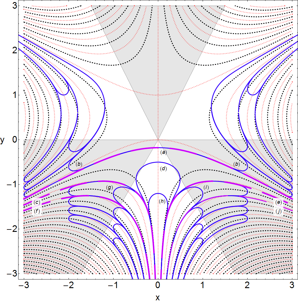
Figure 14: Paths (heavy dashed lines) that connect the left good Stokes’ wedge to the right good Stokes’ wedge for the ground state of the quasi-exactly-solvable ${\cal P}{\cal T}$ anharmonic oscillator whose Hamiltonian is given in (24). There is exactly one such separatrix path (a) that goes directly from the left good wedge to the right good wedge, crossing the imaginary axis at $y=-0.176\,651\,795\,619\,462\,368$. A path (b) that crosses the imaginary axis at a slightly higher point than the (a) path cannot reach $\infty$ in the good Stokes’ wedge. Because they are unstable, such paths turn around, enter the upper bad Stokes’ wedges, and can never re-emerge from these wedges. A separatrix path (c) is shown leaving the left good Stokes’ wedge. This path enters the lower bad Stokes’ wedge to the left of the imaginary axis, re-emerges along paths (d) or (h), and reenters the bad Stokes’ wedge to the right of the imaginary axis. It then continues into the right good Stokes’ wedge along the separatrix (e). Another separatrix path (f) leaves the left good Stokes’ wedge and follows a more complicated course: After entering the lower bad Stokes’ wedge, it leaves and returns along (g), leaves and reenters again along (d) or (h), leaves and reenters along (j), and finally enters the right good Stokes’ wedge along the separatrix (f). Solution paths are horizontal on the lightly dotted lines and vertical on the heavily dotted lines.

VI.2 Probability contours associated with excited states

The eigenfunctions associated with higher energies have nodes in the complex plane. When $J=2$, there is one node. The eigenfunctions have the general form

$$\psi_{n}(x)=e^{-ix^{3}/3-ax^{2}/2}(x+c).$$ (119)

The parameter $c$ is determined by requiring that $\psi_{n}(x)$ satisfy the time-independent Schrödinger equation

$$\left(-\frac{d^{2}}{dx^{2}}-x^{4}+2iax^{3}+a^{2}x^{2}-4ix-E_{n}\right)\psi_{n}(x)=0.$$ (120)

From this Schrödinger equation we obtain two equations, $3a-2ic-E_{n}=0$ and $\left(a-E_{n}\right)c=0$, from which we conclude that the two energy levels and corresponding eigenfunctions are

$$E_{0}=a \psi_{0}(x)=e^{-ix^{3}/3-ax^{2}/2}(x-ia),$$

$$E_{1}=3a \psi_{1}(x)=e^{-ix^{3}/3-ax^{2}/2}x.$$ (121)

The probability contours associated with $\psi_{1}(x)$ for the case $a=1$ are shown in Fig. 15. This figure is quite similar in structure to Fig. 10 for the case of the quantum harmonic oscillator NODE .

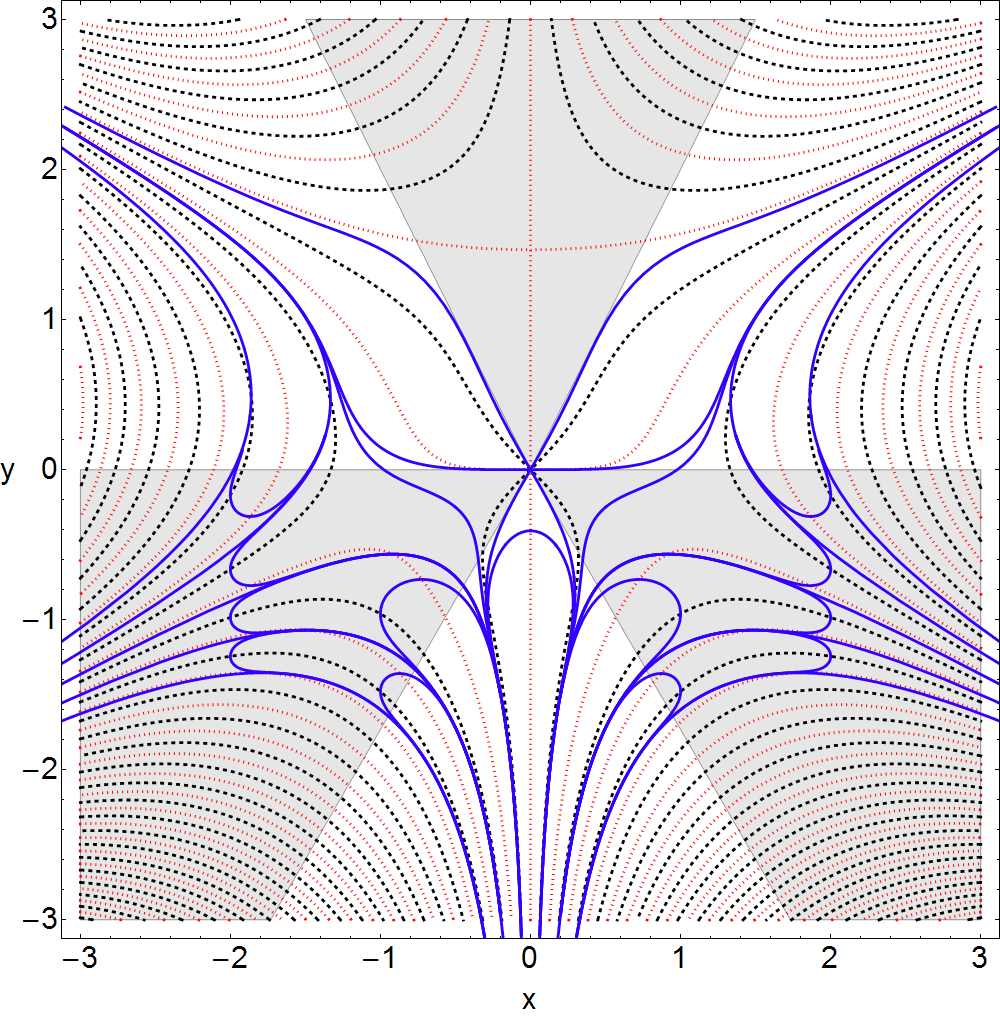
Figure 15: Five paths (heavy solid lines) that emerge from the left good Stokes’ wedge and attempt to reach the right good Stokes’ wedge for the first excited state of the quasi-exactly-solvable ${\cal P}{\cal T}$ anharmonic oscillator whose Hamiltonian is given in (24). The upper two paths veer upward into the bad Stokes’ wedge and die there. The other three paths enter and reenter the lower bad Stokes’ wedge and eventually pass through the node at the origin. Then, these paths repeat this process in the right-half plane and eventually succeed in reaching the right good Stokes’ wedge. Note that there are six paths that enter the node at the origin; the two horizontal paths and the upper two paths eventually wind up in the upper bad Stokes’ wedges. The lower two paths that leave the node enter the lower bad Stokes’ wedge; these paths become part of the complicated route connecting the left to the right good Stokes’ wedges. The solutions to the differential equation are horizontal on the lightly dotted lines and vertical on the heavily dotted lines.

When $J=3$, there are two nodes, and the associated probability contours associated with the highest-energy eigenfunction are shown in Fig. 16. The contours in this figure are qualitatively similar to those in Fig. 11 for the harmonic oscillator.

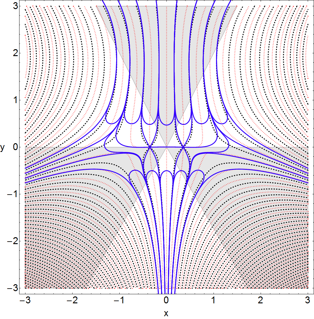
Figure 16: Four paths (heavy solid lines) that emerge from the left good Stokes’ wedge and attempt to reach the right good Stokes’ wedge for the second excited state of the quasi-exactly-solvable ${\cal P}{\cal T}$ anharmonic oscillator whose Hamiltonian is given in (24). The upper two paths veer upward and eventually curve around into the bad Stokes’ wedge and die there. The other two paths enter and reenter the lower bad Stokes’ wedge. After passing through both nodes these paths finally succeed in reaching the right good Stokes’ wedge along separatrix paths. The solutions to the differential equation are horizontal on the lightly dotted lines and vertical on the heavily dotted lines.

As we move to higher energy and there are more nodes, the distribution of eigenpaths begins to resemble the canopy of the classical probability distribution in the complex plane. For the case $J=2$ the classical canopy is shown in Fig. 17.

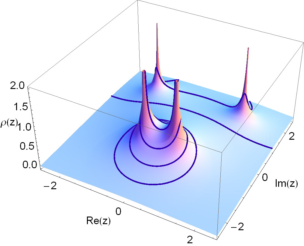
Figure 17: Analog of Fig. 4 for the quasi-exactly-solvable ${\cal P}{\cal T}$-symmetric anharmonic oscillator. The classical probability distribution in the complex plane for the case $J=2$, $a=1$, $E=3$ is shown.

VII Final remarks and future research

In this paper we have shown that it is possible to extend the conventional probabilistic description of quantum mechanics into the complex domain. We have done so by constructing eigenpaths in the complex plane on which there is a real and positive probability density. When this probability density is integrated along an eigenpath, the total probability is found to be finite and normalizable to unity.

There are many generalizations of this work that need to be investigated and much further analysis that needs to be done. To begin with, it is important to understand the time dependence of the complex probability contours. In this paper we have restricted our attention to the eigenpaths associated with eigenfunctions of the Hamiltonian. Such paths are time independent. However, for wave functions that are not eigenfunctions of the Hamiltonian, and even for simple finite linear combinations of eigenfunctions, there is a complex probability current and the probability density flows in the complex plane. We have considered here only one elementary situation in which the complex probability contour is time dependent, and this was for the case of a complex random walk. We believe that a detailed study should be made of the high quantum-number limit; time-dependent contours $C$ for non-eigenstates (such as gaussian wave packets) should be examined; the complex correspondence principle for coherent states should also be developed PPSR .

A second interesting topic for investigation is a detailed comparison of the classical pup tent in Fig. 4 and the analogous quantum picture. The pup tent in Fig. 4 was constructed by making the assumption that all elliptical paths in Fig. 3 were equally likely. But of course this is not quite valid. It is far less likely for a classical particle to be on a large ellipse than on a small ellipse close to the conventional oscillatory trajectory (the degenerate ellipse) on the real axis. A measure of the relative likelihood of being on any given classical ellipse is provided by the standard quantum probability density on the real axis as given in Figs. 1 and 2. Thus, we believe that the probability of being on a large ellipse is exponentially smaller than being on a small ellipse. With this improvement, the probability of a classical particle being somewhere in the complex-$z$ plane can now be normalized to unity. (The volume under the pup tent in Fig. 4 is infinite.)

With these changes in the distribution of classical probability, we can now begin to analyze the global distribution of quantum probability. The improved classical pup tent can now serve as a guide for estimating the relative probability of being on the various eigenpaths shown in Figs. 9, 10, and 11 for the harmonic oscillator, and Figs. 14, 15, and 16 for the quasi-exactly solvable anharmonic oscillator. We expect that the quantum pup tent describing the global distribution of quantum probability in the complex plane will have ripples like the oscillations illustrated in Figs. 1 and 2 of the quantum probability density on the real axis.

Finally, the most important feature of the quantum probability distribution in the complex plane – what we refer to above as the quantum pup tent – is that the density of probability along a complex contour is locally positive. However, the asymptotic analysis in Secs. IV and VI of integration contours entering and leaving the bad Stokes’ wedges leads us to conclude that for the total integral along an eigenpath to be finite some of the contribution to the probability integral must be negative. Our interpretation of this effect is not that the probability density is negative (the integrand is certainly positive), but rather that the contour goes in a negative direction and thus contributes negatively. (A trivial example of such behavior is given by the integral $\int_{1}^{0}dx$. The area under the line $y=1$ is positive, but the integral is negative because it is taken in the negative direction.) This effect is interesting, and we believe that it deserves further examination. The fact that the total probability is unity but that individual contributions to the total probability are both positive and negative is strongly reminiscent of the results found in Ref. PPSS for the Lehmann weight functions for Green’s functions of ${\cal P}{\cal T}$-symmetric field theories. We believe that the ${\cal C}$ operator, which is needed to understand the negative contributions to the Lehmann weight function, will ultimately play a significant role in the future analysis of the complex generalization of quantum probability.

- (1) C. M. Bender, S. Boettcher, and P. N. Meisinger, J. Math. Phys. 40, 2201 (1999).
- (2) A. Nanayakkara, Czech. J. Phys. 54, 101 (2004) and J. Phys. A: Math. Gen. 37, 4321 (2004).
- (3) F. Calogero, D. Gomez-Ullate, P. M. Santini, and M. Sommacal, J. Phys. A: Math. Gen. 38, 8873-8896 (2005).
- (4) C. M. Bender, J.-H. Chen, D. W. Darg, and K. A. Milton, J. Phys. A: Math. Gen. 39, 4219 (2006).
- (5) C. M. Bender, D. D. Holm, and D. W. Hook, J. Phys. A: Math. Theor. 40, F81 (2007).
- (6) C. M. Bender, D. D. Holm, and D. W. Hook, J. Phys. A: Math. Theor. 40, F793-F804 (2007).
- (7) C. M. Bender and D. W. Darg, J. Math. Phys. 48, 042703 (2007).
- (8) A. Fring, J. Phys. A: Math. Theor. 40, 4215 (2007).
- (9) Yu. Fedorov and D. Gomez-Ullate, Physica D 227, 120 (2007).
- (10) P. Grinevich and P. M. Santini, Physica D 232, 22 (2007).
- (11) C. M. Bender, D. C. Brody, J.-H. Chen, and E. Furlan, J. Phys. A: Math. Theor. 40, F153 (2007).
- (12) B. Bagchi and A. Fring, J. Phys. A: Math. Theor. 41, 392004 (2008).
- (13) C. M. Bender and J. Feinberg, J. Phys. A: Math. Theor. 41, 244004 (2008).
- (14) T. L. Curtright and D. B. Fairlie, J. Phys. A: Math. Theor. 41, 244009 (2008).
- (15) A. V. Smilga, J. Phys. A: Math. Theor. 42, 095301 (2009).
- (16) C. M. Bender, F. Cooper, A. Khare, B. Mihaila, and A. Saxena, Pramana J. Phys. 73, 375 (2009).
- (17) P. E. G. Assis and A. Fring, arXiv:0901.1267.
- (18) C. M. Bender, J. Feinberg, D. W. Hook, and D. J. Weir, Pramana J. Phys. 73, 453 (2009).
- (19) C. M. Bender, D. W. Hook, and K. S. Kooner, arXiv:1001.1548.
- (20) C. M. Bender and S. Boettcher, Phys. Rev. Lett. 80, 5243 (1998).
- (21) P. Dorey, C. Dunning, and R. Tateo, J. Phys. A: Math. Gen. 34 L391 (2001); ibid. 34, 5679 (2001).
- (22) A. Mostafazadeh, J. Math. Phys. 43, 205 (2002) and ibid. 2814 (2002).
- (23) C. M. Bender, D. Brody and H. F. Jones, Phys. Rev. Lett. 89, 270401 (2002); ibid. 92, 119902E (2004).
- (24) C. M. Bender, P. N. Meisinger, and Q. Wang, J. Phys. A: Math. Gen. 36, 1973-1983 (2003).
- (25) C. M. Bender, D. Brody and H. F. Jones, Phys. Rev. Lett. 93, 251601 (2004); Phys. Rev. D 70, 025001 (2004).
- (26) C. M. Bender, Contemp. Phys. 46, 277 (2005) and Repts. Prog. Phys. 70, 947 (2007).
- (27) P. Dorey, C. Dunning, and R. Tateo, J. Phys. A: Math. Gen. 40, R205 (2007).
- (28) A. Mostafazadeh, arXiv:0810.5643.
- (29) Z. H. Musslimani, K. G. Makris, R. El-Ganainy, and D. N. Christodoulides, Phys. Rev. Lett. 100, 030402 (2008).
- (30) K. G. Makris, R. El-Ganainy, D. N. Christodoulides, and Z. H. Musslimani, Phys. Rev. Lett. 100, 103904 (2008).
- (31) O. Bendix, R. Fleischmann, T. Kottos, and B. Shapiro, Phys. Rev. Lett. 103, 030402 (2009).
- (32) A. Guo, G. J. Salamo, D. Duchesne, R. Morandotti, M. Volatier-Ravat, V. Aimez, G. A. Siviloglou, and D. N. Christodoulides, Phys. Rev. Lett. 103, 093902 (2009).
- (33) C. E. Rüter, D. Kip, K. G. Makris, D. N. Christodoulides, O. Peleg, and M. Segev, Technical digest, CLEO/IQEC (ISBN: 978-1-55752-869-8), pages: 1-2pages: 183, 2009, IEEE conference proceedings. Presented at: The Conference on Lasers and Electro-Optics and the International Quantum Electronics and Laser Science Conference (CLEO/IQEC), 2009, Baltimore, MD, USA.
- (34) C. E. Rüter, K. G. Makris, R. El-Ganainy, D. N. Christodoulides, M. Segev, D. Kip, Nat. Phys. in press.
- (35) C. T. West, T. Kottos, and T. Prosen, Phys. Rev. Lett., in press.
- (36) M. C. Zheng, D. N. Christodoulides, R. Fleischmann, T. Kottos, submitted.
- (37) L. Pauling and E. B. Wilson, Jr., Introduction to Quantum Mechanics with Applications to Chemistry (Dover, New York, 1985).
- (38) L. I. Schiff, Quantum Mechanics (McGraw-Hill, New York, 1955), Second Ed., Chap. IV, Sec. 13.
- (39) C. M. Bender, D. W. Hook, P. N. Meisinger, and Q. Wang, Phys. Rev. Lett., in press.
- (40) C. M. Bender, D. C. Brody, and D. W. Hook, J. Phys. A: Math. Theor. 41, 352003 (2008).
- (41) C. M. Bender and T. Arpornthip, Pramana J. Phys. 73, 259 (2009).
- (42) J. D. Jackson, Classical Electrodynamics (John Wiley & Sons, New York, 1975), Second Ed., Secs. 7.4 and 8.1.
- (43) C. M. Bender and S. Boettcher, J. Phys. A: Math. Gen. 31, L273 (1998)
- (44) C. M. Bender and S. A. Orszag, Advanced Mathematical Methods for Scientists and Engineers (Springer-Verlag, New York, 1999), Chap. 4 and Prob. 4.13.
- (45) M. V. Berry and C. J. Howls, Proc. Roy. Soc. A 430, 653 (1990).
- (46) M. V. Berry and C. J. Howls, Proc. Roy. Soc. A 434, 657 (1991).
- (47) M. V. Berry in Asymptotics Beyond All Orders, ed. by H. Segur, S. Tanveer, and H. Levine (Plenum, New York, 1991), pp. 1-14.
- (48) There is a fundamental link between quantization of eigenvalues (or of eigenpaths) and hyperasymptotics: As the energy varies, just as it passes through an eigenvalue, one catches a glimpse of the transcendentally small (subdominant) component of the asymptotic behavior of the solution to the time-independent Schrödinger equation. This happens because the coefficient of the exponentially growing solution momentarily passes through zero, and this promotes the exponentially damped solution from hyperasymptotic status to Poincaré asymptotic status.
- (49) In general, all eigenfunctions have nodes. Thus, when , and , have one node each. However, we regard the node of as being unphysical because it is located on the imaginary axis, while the node of is physical because it is located on the real axis. For the general case, the lowest-energy eigenfunction has all nodes on the imaginary axis, and as the energy increases, more and more nodes move off the imaginary axis and become physical. The physical nodes lie on an arch-shaped curve that is symmetric about the imaginary axis. A numerical study of these nodes may be found in C. M. Bender, S. Boettcher, and V. M. Savage, J. Math. Phys. 41, 6381 (2000).
- (50) Coherent states for non-Hermitian -symmetric potentials are discussed in E. M. Graefe, H. J. Korsch, and A. E. Niederle, Phys. Rev . Lett. 101, 150408 (2008).
- (51) C. M. Bender, S. Boettcher, P. N. Meisinger, and Q. Wang, Phys. Lett. A 302, 286 (2002).