One simulation to fit them all - changing the background parameters of a cosmological N-body simulation

Abstract

We demonstrate that the output of a cosmological N-body simulation can, to remarkable accuracy, be scaled to represent the growth of large-scale structure in a cosmology with parameters similar to but different from those originally assumed. Our algorithm involves three steps: a reassignment of length, mass and velocity units, a relabelling of the time axis, and a rescaling of the amplitudes of individual large-scale fluctuation modes. We test it using two matched pairs of simulations. Within each pair, one simulation assumes parameters consistent with analyses of the first-year WMAP data. The other has lower matter and baryon densities and a 15% lower fluctuation amplitude, consistent with analyses of the three-year WMAP data. The pairs differ by a factor of a thousand in mass resolution, enabling performance tests on both linear and nonlinear scales. Our scaling reproduces the mass power spectra of the target cosmology to better than 0.5% on large scales ($k<0.1h{\rm Mpc}^{-1}$) both in real and in redshift space. In particular, the BAO features of the original cosmology are removed and are correctly replaced by those of the target cosmology. Errors are still below 3% for $k<1h{\rm Mpc}^{-1}$. Power spectra of the dark halo distribution are even more precisely reproduced, with errors below 1% on all scales tested. A halo-by-halo comparison shows that centre-of-mass positions and velocities are reproduced to better than $90h^{-1}$kpc and 5%, respectively. Halo masses, concentrations and spins are also reproduced at about the 10% level, although with small biases. Halo assembly histories are accurately reproduced, leading to central galaxy magnitudes with errors of about $0.25$ magnitudes and a bias of about $0.13$ magnitudes for a representative semi-analytic model. This algorithm will enable a systematic exploration of the coupling between cosmological parameter estimates and uncertainties in galaxy formation in future large-scale structure surveys.

1 Introduction

Ever since the first measurements, made almost 40 years ago, the clustering of galaxies has been recognized as a powerful and robust tool to investigate some of the most fundamental questions in cosmology and galaxy formation. Subsequent years have produced major advances on both observational and theoretical fronts, and the study of the three-dimensional distribution of galaxies has contributed enormously to our current understanding of cosmic evolution. For instance, it has provided information about the total matter content of the Universe, the amount of baryons, the formation and evolution of galaxies, and even about the nature of gravity.

The potential to learn from the galaxy distribution is still far from exhausted. New galaxy surveys are scanning ever larger volumes providing more homogeneous and more detailed structural information, and thereby improving considerably the accuracy which can be achieved with existing probes of cosmological physics. In addition, exciting new probes such as the imprint of Baryonic Acoustic Oscillations (BAO, e.g. Eisenstein et al., 2005; Cole et al., 2005; Gaztanaga et al., 2008; Sánchez et al., 2009), the form of redshift-space distortions (Guzzo et al., 2008; Percival & White, 2008), the clustering amplitude of dark matter haloes (Seljak, 2008; Matarrese & Verde, 2008; Carbone et al., 2008) and the evolution of gravitational lensing signals (Huterer et al., 2006; Hoekstra et al., 2006; Berge et al., 2009; Debono et al., 2009) have been proposed to explore, for instance, the nature of the dark energy and the amplitude of primordial non-Gaussianities. In addition, higher-order clustering could provide fresh insights into many of the cosmological issues mentioned above (Baugh et al., 2004; Croton et al., 2007; Ross et al., 2008).

A key step towards achieving optimal exploitation of galaxy clustering data and towards assessing the power of future experiments is to refine our understanding of the connection between galaxy formation and the background cosmological model. In particular, there are two aspects that need to be addressed. The first is the interplay between local baryonic physics and the large-scale evolution of density perturbations (see e.g. Zheng & Weinberg, 2007; Harker et al., 2007). For instance, how different is the efficiency of star formation in a universe with larger dark matter perturbation amplitudes? Can we use the small-scale clustering of galaxies, which is heavily affected by astrophysics, to learn about the underlying cosmological model? Another crucial aspect is to study whether uncertainties in galaxy formation physics will weaken or possibly bias the cosmological constraints extracted from future datasets, e.g. how robust is a measurement of the dark energy equation of state derived from BAO to uncertainties in how (and where) galaxies form (e.g. Angulo et al., 2008)?

In order to explore these issues we require accurate and flexible theoretical predictions for the properties and the spatial distribution of galaxies over large volumes. Currently, the most sophisticated models are built in a three-step process. First, the abundance, structure and clustering of haloes are predicted by following the evolution of the dark matter in a high-resolution N-body simulation (e.g. Springel et al., 2006). Second, the properties of galaxies within these haloes are predicted using either semi-analytic recipes (e.g. Baugh, 2006) or empirically motivated parametric techniques known as halo occupation distribution (HOD) models (e.g. Cooray & Sheth, 2002). Lastly, the appropriate flux limits, sample selection criteria, redshift completeness and survey geometry are applied to build realistic mock catalogues.

Unfortunately, the realism of these mock catalogue implies a substantial computational cost, especially when very large scales are probed. A simulation that resolves simultaneously Gigaparsec scales and Milky-Way sized haloes takes at least several days in the largest supercomputers available today. The modelling becomes even more expensive when one considers that a large number of independent N-body simulations are needed to assess clustering errors properly. An adequate estimation of the variance requires several dozen realizations of the density field (e.g. a $10$% error on a variance estimate for a Gaussian distribution requires $\sim 50$ realizations), and an order of magnitude more simulations are needed to robustly compute the full covariance matrix (Takahashi et al., 2009). In practice, these technical constraints mean that this method can be applied to simulate galaxies only in a very limited number of cosmological scenarios, which then very sparsely sample the allowed cosmological parameter space. This results in an incomplete picture of the coupling between galaxy formation and cosmology.

In this paper we propose and test a new approach which avoids this limitation and allows high-fidelity mock catalogues to be created for a broad range of cosmological scenarios. Current constraints on cosmological parameters, derived from analyses of CMB fluctuations, of supernovae and of galaxy clustering, allow only relatively small variations around the preferred structure formation model (see e.g Sánchez et al., 2009). Taking advantage of this, we explore whether it is possible to manipulate the results of a single N-body simulation to represent the growth of structure (with the accuracy needed for faithful galaxy modelling) over the whole allowed cosmological parameter space. In particular, we will focus on reproducing the position, velocity, abundance and mass of the dark matter haloes thought to host galaxies. Matching these properties accurately at all times ensures a correct merger history for all DM haloes and therefore the correct prediction of the properties of the galaxies within them for any given galaxy formation model. The resulting “scaled” galaxy catalogues thus correspond to those expected in the target cosmology.

Our proposed algorithm consists of the following steps. First, a scaling of the box-size and particle mass together with a reassignment of the output redshifts of the original N-body simulation matches the shape of the linear variance of fluctuations in the target cosmology over the range of scales which give rise to observable nonlinear structure in that cosmology. Second, using linear perturbation theory, the large-scale components of the displacement and velocity fields are corrected to take account of the differences in power spectrum shape between the original and target cosmologies.

The layout of our paper is as follows. In §2 we present more details of our algorithm. We discuss how length, mass and velocity units are altered and the time axis relabelled to match the nonlinear evolution of perturbations. We then describe how to rescale the amplitude of individual long-wavelength modes at each redshift in order to correct the linear and quasi-linear evolution on these scales. In §3.1 we present a suite of N-body simulations specially designed to test the accuracy of our scaling procedure and in §3.2 we use them to show how well the full nonlinear matter power spectrum and its evolution can be reproduced for a chosen cosmology by scaling the particle distribution from a simulation of a different cosmology. The resulting halo catalogues are then compared in §4 with catalogues constructed from a matched simulation carried out directly in the target cosmology. Finally, in §5 we provide a summary and we discuss applications of our method.

2 Scaling an N-body simulation

In this section we will show how it is possible to use the results of an N-body simulation carried out in one cosmology to represent the growth of structure in a different cosmology. For example, how to predict the evolution of structure in a cosmology with the parameters preferred by analyses of the 3rd year WMAP data using the Millennium Simulation, which was carried out using parameters based on an analysis of the 1st year WMAP data. This procedure can be repeated for an arbitrary number of target cosmologies, fully covering the allowed region of the cosmological parameter space for the standard $\Lambda$CDM model. In §2.1 we provide the background and motivation behind our algorithm, and in §2.2 we outline a practical implementation of these ideas.

2.1 Theoretical motivation

Let us denote by $P(k)$ the linear matter power spectrum extrapolated to $z=0$ in our original cosmology (WMAP1 in the example we give below). The linear theory power spectrum at redshift $z$ is then $D^{2}(z)P(k)$, where $D(z)$ is the linear growth factor for this original cosmology in units of its present-day value, i.e. $D(0)=1$. We can now define the variance of the linear density field as a function of smoothing scale through:

$$\sigma^{2}(R,z)\equiv D^{2}\frac{1}{4\pi}\int_{0}^{\infty}{\rm d}kk^{2}P(k)W^{2}(kR)=D^{2}\sigma^{2}_{0}(R)$$ (1)

where $R$ is a comoving smoothing scale, and $W(kR)=3(\sin(kR)-kR\cos(kR))/(kR)^{3}$ is the Fourier transform of the real-space top-hat filter.

For a specific realisation of $P(k)$, the approximation of Zel’dovich (1970) relates Eulerian comoving positions $\mn@boldsymbol{x}$ at redshift $z$ to the corresponding initial, or Lagrangian, comoving positions $\mn@boldsymbol{q}$ through:

$$\mn@boldsymbol{x}(\mn@boldsymbol{q},z)=\mn@boldsymbol{q}-D(z)\mn@boldsymbol{S}(\mn@boldsymbol{q}),$$ (2)

and in this approximation, the peculiar velocities at redshift $z$ are given by:

$$a\dot{\mn@boldsymbol{x}}\equiv\mn@boldsymbol{v}(\mn@boldsymbol{q},z)=-\frac{\dot{D}(z)}{1+z}\mn@boldsymbol{S}(\mn@boldsymbol{q}).$$ (3)

The dots here denote derivatives with respect to time and $\mn@boldsymbol{S}(\mn@boldsymbol{q})$ is the linear displacement field of the realisation extrapolated to $z=0$.

Let us now consider a “target” cosmological model (WMAP3 in our example below) which we seek to study using simulation results obtained within our original cosmological model. In the following, unprimed quantities will continue to refer to the original cosmology, while primed quantities $P^{\prime}$, $D^{\prime}$, $\sigma^{\prime}$, $\sigma^{\prime}_{0}$, $S^{\prime}$ will refer to the target cosmology. Let us assume $z_{\rm f}$ to be the latest time at which the target cosmology must be matched (often $z_{\rm f}=0$). The first step in our procedure is to decide a length scaling from original simulation box-size to target box-size $L^{\prime}=s\,L$. This is defined so that the linear fluctuation amplitude $\sigma^{\prime}(R,z_{\rm f})$ in the target cosmology over the range $[R_{1},R_{2}]$ is as close as possible to that in the original cosmology over the range $[s^{-1}\,R_{1},s^{-1}\,R_{2}]$ at a redshift $z_{*}(z_{\rm f})$. Thus we minimize:

$$\delta_{\tt rms}^{2}(s,z_{*}) = \frac{1}{\ln(R_{2}/R_{1})}\times$$ (4)

$$\int_{R_{1}}^{R_{2}}\frac{{\rm d}R}{R}\left[1-\dfrac{\sigma(s^{-1}\,R,z_{*})}{\sigma^{\prime}(R,z_{\rm f})}\right]^{2},$$

over $s$ and $z_{*}$ (see Zheng et al., 2002; Harker et al., 2007, for a similar approach).

In Press-Schechter theory the halo mass function is determined completely by the variation with scale of $\sigma(R,z)$ the smoothed linear variance of the field. Eq.4 is thus equivalent to minimizing the difference between the halo mass functions in the target and scaled original cosmologies over the (target) mass range $[M(R_{2}),M(R_{1})]$. This sets the range of scales included in Eq.4: $M(s^{-1}R_{2})$ is the mass of the largest halo in the original simulation at $z=z_{*}$ and $M(s^{-1}R_{1})$ that of the smallest resolved halo. For the top-hat filter we are using we have $M(R)=\frac{4\pi}{3}\rho_{0}\,R^{3}$.

We take the original simulation at $z_{*}$ after scaling all lengths by $s$, to be our first approximation to a simulation of the target cosmology at $z_{\rm f}$. Earlier redshifts in the target cosmology ($z>z_{\rm f}$) are then matched to those in the original cosmology ($z>z_{*}$) through:

$$D^{\prime}(z^{\prime})=\frac{D(z)}{D(z_{*})}D^{\prime}(z_{\rm f}).$$ (5)

If needed, peculiar velocities in the target cosmology can be obtained approximately from those in the original cosmology through:

$$\mn@boldsymbol{v}\rightarrow\mn@boldsymbol{v^{\prime}}=s\frac{\dot{D^{\prime}}(z^{\prime})}{\dot{D}(z)}\frac{(1+z)}{(1+z^{\prime})}\mn@boldsymbol{v},$$ (6)

but in practice we use a more accurate procedure which we now describe.

At each redshift in the target cosmology we can define $R_{\rm nl}(z^{\prime})$ through $\sigma^{\prime}(R_{\rm nl},z^{\prime})=1$ or $\sigma_{0}^{\prime}(R_{\rm nl})=1/D^{\prime}(z^{\prime})$. The fluctuations in the target cosmology on all scales larger than $R_{\rm nl}$ (i.e. $k<R_{\rm nl}^{-1}$) are in the linear regime and thus the corresponding displacements and velocities can be corrected for residual differences in power spectrum between the two cosmologies. This is done by subtracting the long wavelength components of the particle position and velocity fields using the Ze’dovich approximation (Eqs. 2 and 3) with the following low-pass-filtered displacement field,

$$D(z)\mn@boldsymbol{S}_{\mn@boldsymbol{k}}(\mn@boldsymbol{q};s^{-1}R_{\rm nl})=\begin{cases}D(z)\mn@boldsymbol{S}_{\mn@boldsymbol{k}}(\mn@boldsymbol{q})&\text{for $|k|<s/R_{\rm nl}$},\\ 0&\text{for $|k|>s/R_{\rm nl}$},\end{cases}$$ (7)

and then adding them back in after scaling each Fourier component of the displacement field by the square root of the ratio of the amplitude of target to original power spectrum,

$$D^{\prime}(z^{\prime})\mn@boldsymbol{S}^{\prime}_{\mn@boldsymbol{k}}(\mn@boldsymbol{q};R_{\rm nl})=\phantom{xxxxxxxxxxxxxxxxxxxxxxxxxxxxxx}$$

$$\begin{cases}D(z)s\left[\dfrac{P^{\prime}(\mn@boldsymbol{k})}{s^{3}P(s\mn@boldsymbol{k})}\right]^{1/2}\mn@boldsymbol{S}_{s\mn@boldsymbol{k}}(\mn@boldsymbol{q})&\text{for $|k|<1/R_{\rm nl}$},\\ 0&\text{for $|k|>1/R_{\rm nl}$},\end{cases}$$ (8)

which is equivalent to the long-range displacement field in the target cosmology. Note that the corresponding velocity fields are derived from these displacement fields through Eq. 3. Also note that, in Fourier space, the low-pass-filtered displacement and velocity fields of the original simulation at $z$ can be calculated from those used to generate the initial conditions.

A similar technique has been previously studied in the literature, although for a different purpose, by Tormen & Bertschinger (1996) and Cole (1997). These authors used linear perturbation theory to add long-wavelength modes to an N-body simulation of limited box-size. As noted by Cole (1997), a naive implementation neglects the coupling of these long-wavelength modes to the smaller-scale perturbations already included in the simulation. This produces systematic and large biases in the internal properties and clustering of haloes, especially massive ones. We note that in our case this problem is considerably alleviated since we impose relatively small changes on the amplitudes of long-wavelength modes. The correct coupling between large and small scales is included automatically to lowest order.

2.2 Implementation

We now describe briefly the steps of a practical implementation of the ideas presented in the previous subsection.

• Calculate the scale factor, $s$, and the redshift $z_{*}$ by minimizing Eq. 4.

• For each output $z>z_{*}$ of the original simulation calculate the corresponding $z^{\prime}(z)$ in the target cosmology using Eq. 5.

  Then for each $z^{\prime}-z$ pair:

• Calculate $R_{\rm nl}$ .

• Calculate $\mn@boldsymbol{S}(\mn@boldsymbol{q};s^{-1}R_{\rm nl})$ for the original simulation.

• Invert $\mn@boldsymbol{x}=\mn@boldsymbol{q}-D(z)\mn@boldsymbol{S}(\mn@boldsymbol{q};s^{-1}R_{\rm nl})$ in the original simulation to obtain $\mn@boldsymbol{q}(\mn@boldsymbol{x};s^{-1}R_{\rm nl},z)$. This can be done recursively:

  $$\mn@boldsymbol{q}_{i}=\mn@boldsymbol{x}-D(z)\mn@boldsymbol{S}(\mn@boldsymbol{q};s^{-1}R_{\rm nl})$$ (9)

  with $\mn@boldsymbol{q}_{0}=\mn@boldsymbol{x}$ as the starting condition and requiring that $|\mn@boldsymbol{q}_{i}-\mn@boldsymbol{q}_{i-1}|<0.01h^{-1}{\rm Mpc}$, for example, for convergence.

• Remove low-pass-filtered displacement and velocity fields from the original simulation data at redshift $z$.

• Scale to the target cosmology:

• Box size: $L\rightarrow L^{\prime}=sL$.

• Redshift: $z\rightarrow z^{\prime}$.

• Particle mass:

  $$m_{\rm p}\rightarrow m_{\rm p}^{\prime}=\frac{\Omega_{\rm m}^{\prime}H^{\prime 2}L^{\prime 3}}{\Omega_{\rm m}H^{2}L^{3}}m_{\rm p}.$$ (10)

• Residual nonlinear velocities:

  $$\mn@boldsymbol{v}\rightarrow\mn@boldsymbol{v}^{\prime} = \left[\frac{L}{(1+z)m_{\rm p}}\frac{(1+z^{\prime})m_{\rm p}^{\prime}}{L^{\prime}}\right]^{1/2}\mn@boldsymbol{v},$$ (11)

  $$= \left[\frac{\Omega_{\rm m}^{\prime}H^{\prime 2}L^{\prime 2}(1+z^{\prime})}{\Omega_{\rm m}H^{2}L^{2}(1+z)}\right]^{1/2}\mn@boldsymbol{v},$$ (12)

  where unprimed and primed cosmological parameters are present-day values in the original and target cosmologies, respectively.

• Compute new long-range displacement and velocity fields by scaling the Fourier components of the original fields according to Eq. 8 using the power spectra of the two cosmologies. Using the Zel’dovich approximation, add these low-pass filtered fields to the scaled positions and velocities of the particles.

3 Numerical simulations

In this section we provide details of the N-body simulations used to illustrate and probe the accuracy of our algorithm. First, we describe the numerical and cosmological parameters of our simulations, which were carried out at two different resolutions and in two different cosmologies. Next, we discuss how we apply our algorithm to these simulations to test our scaling procedures.

	$m_{\rm dm}$	Box	$\Omega_{\rm m}$	$\Omega_{\rm b}$	h	$\sigma_{8}$
	[$h^{-1}~{}$M⊙]	[Mpc/h]
W1	$3.34\times 10^{11}$	$865.16$	0.250	0.045	0.73	0.9
hW1	$3.34\times 10^{8}$	$86.516$	0.250	0.045	0.73	0.9
W3	$4.92\times 10^{11}$	$1000.0$	0.238	0.0416	0.732	0.761
hW3	$4.92\times 10^{8}$	$100.0$	0.238	0.0416	0.732	0.761

Table 1: The values of some of the basic parameters used in the simulations. The columns are as follows: (1) The name of the simulation. (2) The mass of a dark matter particle. (3) the side of the computational box (4) The matter density. (5) The baryon density. (6) The Hubble parameter in units of 100 kms/s/Mpc. (7) The linear fluctuation amplitude at $z=0$, $\sigma_{8}$. In both cases, the primordial spectral index is $n_{s}=1$ and the dark energy is assumed to be a cosmological constant.

3.1 Direct N-body Simulations

In this paper we compare results from cosmological simulations at two very different resolutions: large-volume simulations are used to study the performance of our algorithm in reproducing large-scale structure; smaller volume but higher resolution simulations are used to study its performance in reproducing the properties of individual dark matter haloes. The latter simulations are also used as input to a semi-analytic model for galaxy formation which allow us to compare the properties of the galaxies predicted in our scaled and true simulations.

The first of our two cosmologies is that of the Millennium Simulation (Springel et al., 2005) and is consistent with an analysis of the 1st year of data from the WMAP satellite (Spergel et al., 2003). The corresponding large and small volume simulation are labelled as W1 and hW1, respectively. The second cosmology corresponds to an analysis of the 3rd year WMAP data (Spergel et al., 2007; Sánchez et al., 2006), and we refer to the large and small volume simulations as W3 and hW3, respectively. The specific values of the parameters for the two models can be found in Table 1.

Each of our four simulations contains $512^{3}$ dark matter particles. For the W3 simulation the size of the box is $L^{\prime}=1000h^{-1}{\rm Mpc}$ and the redshifts at which we store the particle data are $z^{\prime}=(0,0.5,1.0,2.0)$. For W1 the corresponding values are $L=865.164h^{-1}{\rm Mpc}$ and $z=(0.57,1.09,1.68,2.92)$. These figures were set so that at each output the respective box sizes and linear amplitude of fluctuations minimize Eq. 4 as described in §2.1 for $[R_{1},R_{2}]=[1,10]h^{-1}{\rm Mpc}$. The hW1 and hW3 simulations have the same cosmological parameters as W1 and W3, but have a 10 times smaller box and 1000 times smaller particle masses.

The starting redshifts are $z=60.0$ and $z=78.08$ for the W1 and W3 simulations, respectively. The Plummer-equivalent softening length has the same value in units of the respective box sizes, $\epsilon=L/10000$. The linear power spectrum is calculated for each cosmology using the CAMB package (Lewis et al., 2000). The initial density fields are generated using the Zel’dovich approximation to perturb a set of particles initially distributed on a cubic grid. Finally, all simulations were evolved with a memory efficient version of the Gadget2 code (Springel, 2005).

We note that the random number sequence used to set initial perturbation amplitudes and phases was the same in the two different cosmologies simulated at each resolution. This allows us to study subtle differences in the final halo and matter distributions and provides stringent and clean tests for our algorithm.

3.2 Scaled Simulations: the algorithm in action

Figure 1: The linear mass variance $\sigma^{2}(M)$ smoothed with a real-space top-hat filter as a function of the smoothing radius for various cosmologies. Symbols in the upper panel show the expected values for our standard WMAP1 (black squares) and WMAP3 (red triangles) cosmologies, and for two cosmologies where all WMAP3 parameters are retained except that $\Omega_{m}$ is raised to 0.4 (blue triangles) and reduced to 0.1 (green triangles). The continuous lines all derive from the WMAP1 cosmology but in the red, green and blue cases our scaling in length and our reassignments of time have been applied in order to match the corresponding “WMAP3” model as well as possible over the range $1h^{-1}{\rm Mpc}<R<10h^{-1}{\rm Mpc}$. The quality of these fits is better appreciated in the bottom panel which shows the difference between symbols and curves as a percentage.

Figure 2: Constraints on $s$ and $D(z_{*})$ obtained by minimizing the logarithmic difference between the WMAP3 and scaled WMAP1 linear variances over the scale range corresponding to resolved haloes in the WMAP3 cosmology. Contours displayed by solid, dotted and dashed lines indicate the regions in parameter space that produce rms deviations smaller than $1$, $10$ and $20\%$. over this mass rangee (see bottom panel of Fig. 1).

In this section we give details of how the hW1 and W1 simulations were scaled and perturbed, according to the algorithm described in §2, to predict the dark matter clustering and the halo properties expected in the cosmological model of the W3 and hW3 simulations.

The first step in our procedure is to scale comoving positions and to re-label redshifts. As discussed in §2.1, this requires finding a new box-size $L^{\prime}$ and redshift $z_{*}$ for the outputs of hW1 and W1 that best reproduce the linear mass variance at $z=0$ of the target WMAP3 cosmology on resolved nonlinear mass scales.

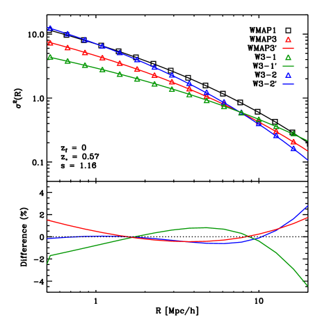
Linear variance is displayed as a function of scale for the original (WMAP1) and target (WMAP3) cosmologies in the upper panel of Fig. 1, together with the best fit of the WMAP1 variance to the WMAP3 variance after scaling lengths and times (see Eq. 4). The range of smoothing radii used in the fit is $[1-10]h^{-1}{\rm Mpc}$ in the WMAP3 cosmology, corresponding to $[10^{11}-10^{15}]\,h^{-1}M_{\odot}$ for our assumed top-hat filter in real space. This is the halo mass range expected to host the galaxies observable in future spectroscopic surveys.

In the bottom panel of Fig. 1 we can see the quality of the fit. Over the scales included in the minimization, the mass variance in the scaled cosmology differs from that in the target cosmology by less than $1\%$. This deviation implies a less than $5\%$ difference in the expected number of “$3\sigma$” haloes between the target simulation and the scaled one, assuming that the mass function of haloes is well described by the Press & Schechter (1974) model.

The potential of our algorithm is further illustrated by the blue and red lines in Fig. 1, which show the results of scaling the WMAP1 variance to match the variance in two more distant cosmologies. $\Omega_{m}$ is set to $0.1$ and $0.4$ in the red and blue cases, respectively, with the remaining parameters kept at their WMAP3 values. For both cases our scaling of WMAP1 reproduces the linear variance of the “WMAP3” model satisfactorily and at a level comparable to the fit of the real WMAP3 cosmology, although, the scaling of box size and the relabeling of redshift is more drastic, as expected. The values for $s$ are $3.47$ and $0.536$, and for $D(z_{*})$ are $0.416$ and $1.311$ for lower and higher $\Omega_{m}$, respectively.

The contour lines in Fig. 2 show the constraints on $s$ and on $D(z_{*})$ for our standard WMAP1-WMAP3 scaling. The best fit values are $s=1.156$ and $D(z_{*})=0.764$ (corresponding to $z_{*}=0.57$). The solid, dotted and dashed lines enclose regions in this two-dimensional parameter space which give rms differences below $1$, $10$, and $20\%$ respectively, between the scaled WMAP1 variance and the WMAP3 variance over the range $[R_{1},R_{2}]$ (see bottom panel of Fig. 1).

Fig. 2 illustrates the degeneracy between these two parameters. The banana-like shape of the contours is, in fact, useful because it gives some latitude in choosing which $s_{*}$, in the original cosmology should correspond to $z=0$ in the target cosmology, allowing one to choose $z_{*}$ to correspond to one of the stored outputs.

For the second part of our algorithm we have produced low-pass-filtered displacement and velocity fields for the WMAP1 and WMAP3 cosmologies on a $512^{3}$ grid as described in §2.2. As discussed previously, at each redshift we included only the contribution of linear modes with $k<R_{nl}^{-1}$. For $z=0$ this criterion implies $k<0.23\,h{\rm Mpc^{-1}}$, while at $z=2$ it implies $k<1.01\,h{\rm Mpc^{-1}}$. This corresponds approximately to smoothing the displacement fields with top-hat filters of radii $4.3\,h^{-1}{\rm Mpc}$ and $0.98\,h^{-1}{\rm Mpc}$, respectively.

For the specific simulations we consider in this paper, our results imply that if we expand the $z=0.57$ outputs of W1 and hW1 by a factor of $1.156$, and then apply the computed large-scale corrections, the results should be almost identical to the W3 and hW3 simulations at $z=0$. Below we refer to these resulting scaled catalogues as W3^′ and hW3^′ and we examine in detail how close they are to W3 and hW3, respectively.

4 COMPARISON WITH DIRECT N-BODY SIMULATIONS

In this section we assess the accuracy of our procedure by comparing the properties of dark matter, halo and galaxy catalogues derived from the scaled W3^′ and hW3^′ simulations with similar catalogues derived from the true W3 and hW3 simulations.

Figure 3: Comparison of the dimensionless power spectrum, $\Delta^{2}(k)=k^{3}P(k)/2\pi^{2}$, measured in the W3 simulation with those of the W1 simulation after different types of scaling. Note that in panel (a) the redshift-space spectra have been offset by 1 dex for clarity. Poisson shot-noise level. Black and brown lines show the power spectra of the dark matter in the W3 and W1 simulations, respectively (note that we show the W1 simulation at $z=0.57$ and that the black dashed line lies behind the dashed blue line). Red lines show the result of scaling up the amplitude of the W1 simulation at $z=0.57$ to match the linear amplitude of perturbations in spheres of $8h^{-1}{\rm Mpc}$. Green lines display the spectrum after scaling both the simulation box and the redshift. In both cases, velocities have been scaled according to Eq. 6. Finally, blue lines illustrate the result of including our linear theory correction in addition to the length and redshift scalings. The deviations after applying the different procedures can be better appreciated in panels (b), (c) and (d), which show the fractional difference $\Delta^{2}_{\tt W1}(k)/\Delta^{2}_{\tt W3}(k)-1$. In each of the four panels, power spectra computed in real and redshift space are displayed as solid and dashed lines respectively.

4.1 Mass clustering

Figure 4: The distribution of the differences in x-coordinate for dark matter particles before (dashed lines) and after (solid lines) our large-scale correction is applied. Different colours show results at different redshifts.

Figure 5: Relative difference, $\Delta^{2}_{\tt W3^{\prime}}(k)/\Delta^{2}_{\tt W3}(k)-1$, between the dimensionless dark matter power spectra measured in the scaled and true simulations as a function of redshift. Solid lines compare W3^′ and W3 and dashed lines hW3^′ and hW3. Black curves refer to real-space and red to redshift-space power spectrum. In each panel, the arrow indicates the wavelength, $k_{nl}$, that satisfies $\Delta^{2}(k_{nl})=1$. This is the largest $k$-value included in our linear theory corrections. The legend in each panel indicates the redshifts of the original (W1) and target (W3) simulation outputs.

Figure 6: The mass density field in a slice of thickness $50h^{-1}{\rm Mpc}$ and side $1000h^{-1}{\rm Mpc}$ at $z=0$ for the W3 (left column) and the W3^′ simulations (middle panel). The difference between these two maps is shown at greatly enhanced contrast in the right column. From top to bottom, the dark matter field has been smoothed with Gaussians of radius $2$, $5$ and $20\,h^{-1}{\rm Mpc}$. The intensity of each pixel is proportional of the logarithm of the density.

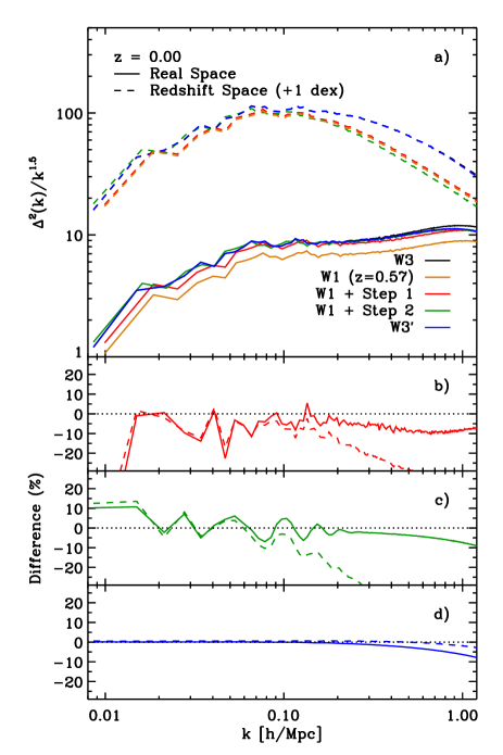
We start testing our algorithm by examining the spatial distribution of dark matter particles. Fig. 3 shows the dimensionless power spectra, $\Delta^{2}=k^{3}P(k)/2\pi^{2}$, in real and redshift space, measured in the W3 simulation and in the W1 simulation after three different scaling procedures have been applied. (The power spectra were computed by assigning particles onto a $512^{3}$ grid using the Cloud-in-Cell scheme, and then Fast Fourier Transforming.)

The first scaling (red lines) consists of adjusting, in a scale-independent way, the linear amplitude of fluctuations in spheres of $8h^{-1}{\rm Mpc}$ of the $z=0.57$ output of W1 to match the fluctuations of the $z=0$ output of W3. The second scaling (green lines) includes a rescaling of the box size in addition to the relabeling of the time variable as described in §3.2. In these two cases, the velocities were scaled according to Eq. 6. The third scaling (blue lines) uses the linear-theory corrections on large scales and thus represents our algorithm in full.

As can be appreciated in the top panel of Fig. 3, all the described procedures perform moderately well, at least on real space. However, the closer look given in the lower sub-panels reveals the deficiencies of each of them. For the simple amplitude scaling, panel (b) shows that differences reach $20\%$ even on scales comparable to the fundamental mode of the simulation box. As the phases in the two simulations coincide in units of box size (and not in units of $h^{-1}{\rm Mpc}$), the ratio is very noisy. As shown in panel (c), these stochastic fluctuations disappear when our length and time scalings are applied. Nevertheless, a strong disagreement persists and an overestimation of nearly $10\%$ remains in the real-space and redshift-space clustering on large scales. These differences result from the different overall shape of the linear theory spectra of the W1 and W3 simulations, and from the fact that we have normalised them to agree on nonlinear scales. In addition, the residuals in panel (c) show an oscillatory pattern. This is a consequence of the different BAO wavelength in the target and scaled simulations, a reflection in part of the different $\Omega_{\rm b}$, but mostly of the rescaling in length. The last panel (d) demonstrates that these large-scale features are efficiently removed by our linear correction procedure.

As can be seen also in panels (b) and (c) of Fig. 3, the velocity scaling of Eq. 6 does an extremely good job in matching streaming motions (and thus the redshift-space power spectra) on large scales, but fails for $k>0.1h{\rm Mpc^{-1}}$ because it is inappropriate for nonlinear quasi-virialised motions. Panel (d) shows that our preferred correction on these scales (Eq. 12) does a much better job.

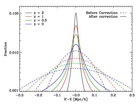
As we show in Fig. 4, after our large-scale correction the 1D rms difference between the position of particles in the true and “scaled” simulations is $0.038h^{-1}{\rm Mpc}$ at $z=0$. This is a factor of $5$ smaller that the rms difference if only the length and time scalings are performed ($0.197h^{-1}{\rm Mpc}$). At higher redshifts the improvement provided by our large-scale correction is even greater. For instance, at $z=2$ it reduces the differences in each dimension by a factor of $10$; the rms values are $0.072$ $h^{-1}{\rm Mpc}$ and $0.0073$ $h^{-1}{\rm Mpc}$ before and after correction, respectively.

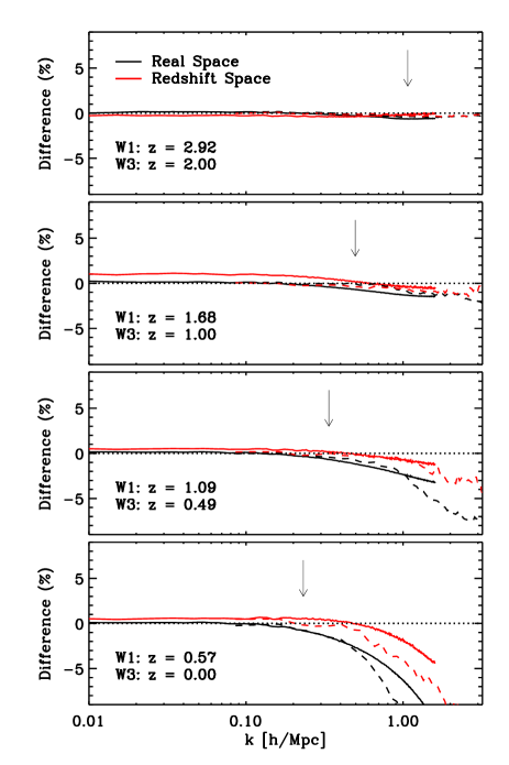
We examine the performance of our full scaling scheme at different redshifts in Fig. 5. Over the range of scales displayed, the dark matter power spectrum of the W3 and W3^′ simulations are in very good agreement. At almost all redshifts the deviations on very large scales ($k<0.1h{\rm Mpc^{-1}}$) are of order $0.2\%$ or less. On smaller scales the amplitude is systematically lower in the scaled dark matter distribution, a discrepancy which gets larger at lower redshift. This small difference ($5\%$ in real space and $10\%$ in redshift space at $k\sim 1h{\rm Mpc^{-1}}$) is due to differences in the halo mass-concentration relations. In the standard picture for structure formation, the concentration of a halo is related to the mean density of the Universe at the time of its formation (which is usually defined in terms of its mass accretion history). Even though our true and scaled cosmologies have, by construction, the same perturbation amplitudes at matched redshifts, their growth histories differ when expressed in terms of redshift. Thus the mean collapse redshift of haloes of given mass will also be different (Dolag et al., 2004; Jennings et al., 2009). As we will see below, this implies that haloes in the scaled simulations are less concentrated than in the true simulations. The effect increases with decreasing redshift reaching $10\%$ by $z=0$. On the other hand, the absence of wiggles in the residual around the BAO scale implies that our Zel’dovich-based corrections do appropriately compensate not only for the linear signal but also, at lowest order, for its nonlinear degradation.

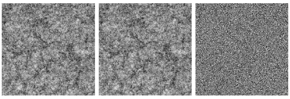
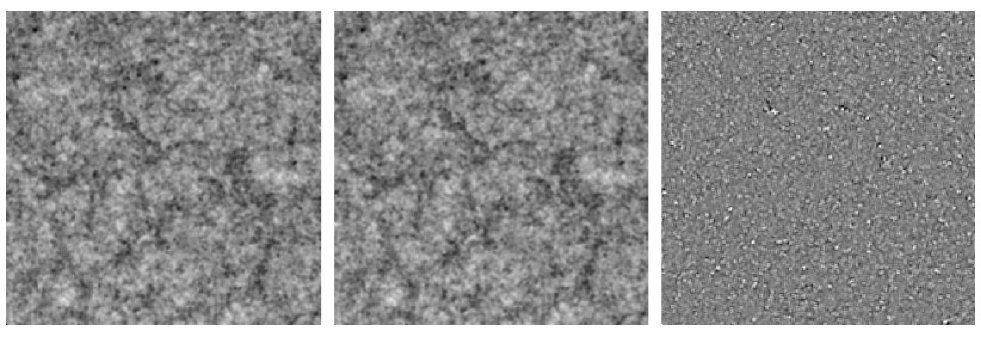
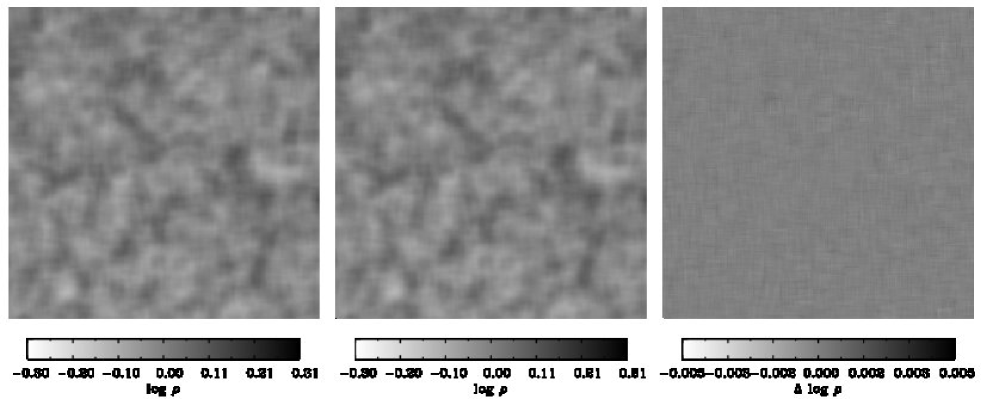
A visual impression of the quality of the scaling is given by Fig. 6. This figure shows the dark matter density field in real space at $z=0$ measured in $50h^{-1}{\rm Mpc}$ slices through the W3 (left column) and W3^′ (central column) simulations. Underdense regions are lighter while clusters and filaments are darker The differences between the two maps are displayed with enhanced contrast in the right column. The density fields have been smoothed with Gaussian kernels of radius $r_{0}=$ $2$, $5$ and $20$ $h^{-1}{\rm Mpc}$ (top, middle and bottom rows respectively). In this way we accentuate the differences between the dark matter fields on different scales.

In every row, we can see that the two simulations have identical structures - voids, filaments and clusters are found at exactly the same locations. Small scales, best seen in the upper panel, show a slight positive bias in dense regions which results from the higher concentration of dark matter haloes in the true W3 simulation than in the scaled W3^′ simulation. Small shifts in the position of clusters appear as black-white dipoles in the right column. The discrepancies between the maps are small in all cases and are strongly reduced when we smooth more strongly. In the bottom row the two fields are virtually indistinguishable. This is consistent with our power spectrum analysis: the matching procedure performs remarkably well on large scales but does not perfectly reproduce the small-scale nonlinear clustering.

4.2 The properties of DM haloes

Figure 7: Comparison of the comoving number density of FoF haloes. We plot the multiplicity function $\rho^{-1}M^{2}{\rm d}N/{\rm d}M$ where $\rho$ is the mean density of the Universe. The curves, from top to bottom, represent redshifts $z=0$, $0.5$ and $1.0$. Solid lines display measurements from the direct simulations hW3 and W3 while dashed lines show results from the scaled catalogues W3^′ and hW3^′. Vertical dotted lines indicate the 100 particles limit for the hW3 and W3 simulations. The lower panel shows the difference “scaled”-true as a percentage.

Figure 8: The distribution of the differences in position, velocity modulus, mass and concentration for FoF haloes at $z=0$ in W3 and W3^′ (dotted lines) and in hW3 and hW3^′ (solid lines). Results are shown for $6$ disjoint mass ranges. Black, red and green curves show distributions for haloes with $[200,700]$, $[700,1500]$ and $>1500$ particles in W3 and hW3. The standard deviation of the distributions is given in the legend of each panel.

Figure 9: Comparison of the concentration (left panel) and of the spin parameter (right panel) for haloes identified in the true (unprimed) and scaled (primed) simulations at $z=0$. For clarity, we have plotted the result only for haloes containing more than $500$ particles. The red lines indicate the result expected if there were no systematic biases between the halo properties in our two simulations (i.e. the one-to-one relation), while the blue lines indicate the straight line that minimises the rms perpendicular residuals.

Figure 10: Relative difference, $\Delta^{2}_{\tt W3^{\prime}}(k)/\Delta^{2}_{\tt W3}(k)-1$, between the dimensionless halo power spectra measured in the scaled and true simulations as a function of redshift. We have used only matched FoF haloes with at least $50$ particles in W3. This limit corresponds to a mass of $2.6\times 10^{12}h^{-1}M_{\odot}$ in the WMAP3 cosmology. The bias of the sample, defined as the mean value of $b=\sqrt{\Delta^{2}_{\rm h}(k)/\Delta^{2}_{\rm dm}(k)}$ on scales $k<0.1h{\rm Mpc^{-1}}$, is shown in the legend of each subpanel and is seen to vary strongly with redshift.

Figure 11: The K-band luminosity function at $z=0$ constructed from the hW3 (green squares) and hW3^′ simulations (red triangles). For comparison, we have also included the luminosity function of the 2dFGRS galaxies as computed from Cole et al.(2001).

We now compare the distribution of dark matter haloes in the true (W3) and scaled W3^′ simulations. These catalogues were built using a FoF group finder (Davis et al., 1985) with a linking length equal to $20\%$ of the mean interparticle separation, which approximately selects objects with $200$ times the mean density. At $z=0$ the number of haloes with at least $50$ particles in the W3 and W3^′ catalogues is $138,284$ and $131,356$, respectively. These figures are $109,651$ and $109,176$ for the hW3 and hW3^′ catalogues.

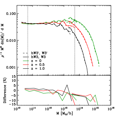
Fig. 7 shows the abundance of dark matter haloes as a function of mass in our two simulations. Over the mass range covered by the catalogues, the mass functions are in very good agreement. Differences are below $10\%$ over $4$ orders of magnitude in mass and over $7$ orders of magnitude in number density! However, focusing on the bottom panel, where differences between the curves can be seen in more detail, it is evident that there are significant systematic discrepancies.

The scaled simulations W3^′ and hW3^′ seem to underpredict the abundance of haloes compared to the W3 and hW3 simulations, or equivalently, FoF masses are systematically higher in the true simulations than in the scaled simulations. In particular, the difference in abundance seems larger for high-mass haloes, this explains the fact that the total number of haloes differs by $5\%$ between W3 and W3^′, but only by $0.5\%$ between hW3 and hW3^′. There are a number of possible reasons for this disagreement. A $\sim 5\%$ disagreement is expected due to the residuals in the mass variance fitting (See Fig. 1). In addition, a fixed linking length identifies objects with lower mean overdensities relative to the mean density if their concentrations are lower, therefore underestimating the mass of objects identified at low redshift. Finally, an important assumption of our work is that the halo mass function is universal (i.e. independent of redshift, cosmological parameters, etc) when the masses are expressed in terms of $\delta_{c}/\sigma(M)$, as predicted by Press-Schechter theory. However, recent simulation results suggest that this picture may work no better than $10\%$, and that properties of the density field other than the shape of the linear variance as a function of smoothing radius may be important (Tinker et al., 2008; Manera et al., 2009).

In order to provide a more detailed comparison between our catalogues we have matched individual haloes in W3^′ and W3. We do this by selecting all the DM particles that belong to each halo with more than $50$ particles in W3 and then finding the halo that contains most of these particles in W3^′. Due to statistical fluctuations not every halo in the W3 (hW3) catalogue can be matched to one in the W3^′ (hW3^′) catalogue. Nevertheless, of the $138,284$ ($109,651$) haloes with more than $50$ particles in W3 (hW3), only $16$ ($21$) are unmatched to a halo with at least $20$ particles in W3^′ (hW3^′).

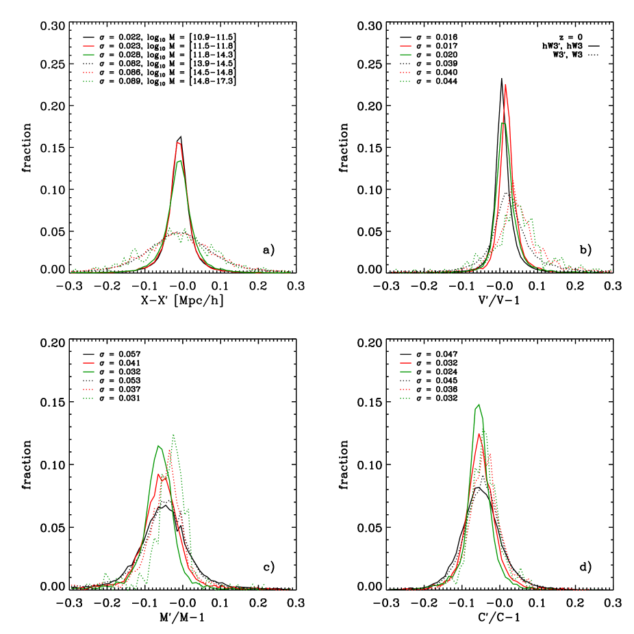
The object-by-object comparison that results from this matching is presented in Fig. 8. In this plot we present the distribution of differences in the position, velocity, mass and concentration of matched FoF haloes for the W3-W3^′ (dotted lines) and for the hW3-hW3^′ catalogues (solid lines). We show the results at $z=0$ and for haloes in $6$ different mass ranges, but we have checked that our results behave in a similar way at different redshifts, and for other mass ranges.

In the top left panel we can see that the centre of mass positions of the FoF haloes, agree remarkably well. For each of the 3 spatial coordinates, discrepancies are typically $85$ $h^{-1}{\rm kpc}$ between the $1h^{-1}{\rm Gpc}$ simulation, but only $30$ $h^{-1}{\rm kpc}$ between the $100h^{-1}{\rm Mpc}$ simulations. These uncertainties are less than half the typical virial radii of the haloes. This agrees with the small differences seen in Fig.6. We note that these differences increase roughly by a factor of two if our large-scale correction is not included. In panel (b) we display differences in the 1D velocity modulus ($V^{2}=V_{x}^{2}+V_{y}^{2}+V_{z}^{2}$) of the centre of mass of our haloes. We find that this quantity is also matched very accurately: better than $\sim 5\%$ rms, and with no measurable bias for both pairs of simulations in all the mass bins inspected.

On the other hand, the FoF masses are slightly less precise. The uncertainty in our scaled halo mass is just under $10\%$ with a systematic underestimation of $\sim 5\%$. We also note that the accuracy at which we match this is greater for our high-resolution simulations.

In contrast, in panel (d), we compare concentrations of FoF haloes using the ratio $C=V_{\rm max}/V_{200}$, where $V_{\rm max}$ is the maximum circular velocity of the main subhalo of the FoF halo and $V_{200}$ is the circular velocity at $R_{200}$, the radius enclosing a mean density 200 times the critical value. The discrepancies here are typically larger in the high-resolution pair, although still under 10% with a bias of about $5\%$. The lower mean concentration of haloes in W3^′ is responsible for the underestimation of the real-space power spectra on small scales seen in Fig. 5. We expect this to impact the spatial distribution of galaxies, if at all, only on very small scales.

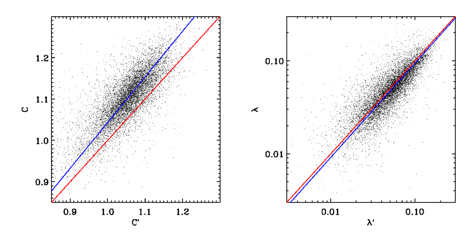
In Fig. 9 we show the accuracy with which our scaling procedure is able to reproduce two important properties of dark matter haloes. In the left panel we compare concentrations (as defined above) of haloes identified in the scaled ($C^{\prime}$) and true simulations ($C$). In agreement with Fig. 8, there is a small bias in the average value which results from differing halo growth with redshift in our two simulations: the concentration of a halo is underestimated by $0.04$ in the scaled simulations. In the right panel we compare the spin parameter defined as $\lambda=\mn@boldsymbol{J}/(\sqrt{2}M_{200}V_{200}R_{200})$ where $\mn@boldsymbol{J}$ is the halo angular momentum and $M_{200}$ is the total mass (both within $R_{200}$) (Bullock et al., 2001). This panel demonstrates that, albeit with scatter, spins are well reproduced by our velocity and position scaling.

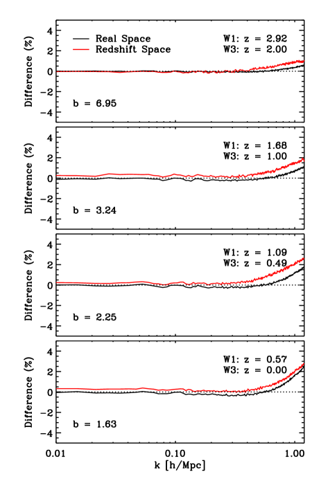
We now explore whether the differences displayed in Fig. 8 and Fig. 9 produce a noticeable effect on halo clustering by comparing the power spectra of the matched catalogues. Fig. 10 presents results in real space (black lines) and in redshift space (red lines) at $z=0$, $0.5$, $1$ and $2$. As found above for the dark matter catalogues, on large scales the two halo power spectra are almost identical. In real space the differences are less than $0.1\%$ while in redshift space they are still below the percent level. This behaviour repeats at all redshifts. On smaller scales, haloes in W3^′ tend to be more clustered than their counterparts in W3. Overall, the distributions agree, over all relevant scales, within $1\%$, an uncertainty much smaller than those likely to be introduced by our poor knowledge of the galaxy formation process.

It is important to note that in these measurements we have used haloes above a fixed mass. As a result, the samples displayed at different redshifts correspond to peaks of different height in the density field, as illustrated by the bias values given in each panel of Fig. 10. Thus, the fact that we recover the expected clustering at all redshifts suggests that the bias-mass relationship is very well reproduced by our algorithm, even for very rare peaks.

Figure 12: The differences in K-band absolute magnitude for central galaxies in the hW3 and hW3^′ catalogues. These galaxies represent the $\sim 56\%$ of all the galaxies with $M_{K}-5\log_{10}h<-18$ in our semi-analytic catalogues. The median of the distribution for the sample as a whole is $0.135$ while the dispersion is $0.233$.

4.3 Models for galaxy formation

The final step in the creation of galaxy mock catalogues is to connect the predictions for dark matter haloes with the observable properties of the galaxies which they host. For this, a crucial requirement is the construction of accurate merger histories. Thus we now explore how well our algorithm performs in this respect (see Neistein et al., 2009, for an attempt to describe merger histories in a cosmology-independent way). We do this by comparing the galaxies built using hW3^′ with those built using an identical procedure on hW3.

There are several different approaches to create realistic galaxy populations in the dark matter haloes of N-body simulations. Here we use so-called semi-analytic models of galaxy formation in which the key physical processes that determine the properties of galaxies are followed from very early times in a self-consistent way within the hierarchically growing halo population. Such semi-analytic modelling represents a hard test for our algorithm since the final properties of galaxies depend not only on the present-day mass of their host haloes but also on their whole assembly histories – merger rates, progenitor mass function, formation times, spins – and indirectly on the properties of the environment that affect these quantities.

The specific model we use in this paper is that developed by the Munich group as described in De Lucia & Blaizot (2007), with the parameters of Wang et al. (2008). This model roughly reproduces the observed $z=0$ K-band luminosity function (among other galaxy properties) in the WMAP3 cosmology, and is adequate for our tests. For both hW3 and hW3^′ we have generated halo merger trees with the same time resolution as in the Millennium Simulation, i.e. roughly $300$ Myr for $z<1$. All levels in the two merger trees are set to correspond appropriately after scaling lengths and masses and reassigning redshifts. This involves matching outputs in the hW3 and the original hW1 simulations as above.

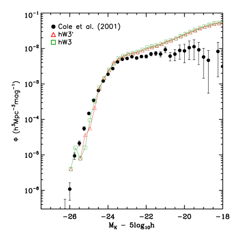
The present-day K-band luminosity functions computed by this model are shown in Fig.11. The green triangles refer to galaxies in the true model hW3, while the blue squares refer to galaxies in the scaled model hW3^′. For comparison we have also included the observed luminosity function from Cole et al. (2001). In both cases our galaxy samples are complete down to $M_{K}-5\log h=-18$. Above this magnitude threshold the catalogues contain $76562$ and $71652$ galaxies for hW3 and hW3^′, respectively. Overall the agreement is quite impressive, especially if one remembers that we are comparing results for simulations run with significantly different sets of cosmological parameters. However, discrepancies exist: there is a small underestimate of the number of galaxies brighter than a given magnitude in the hW3^′ catalogue. This difference is weakly magnitude-dependent and reaches $5\%$ at the faintest magnitudes. It is consistent with the differences in the halo mass function seen in Fig. 7.

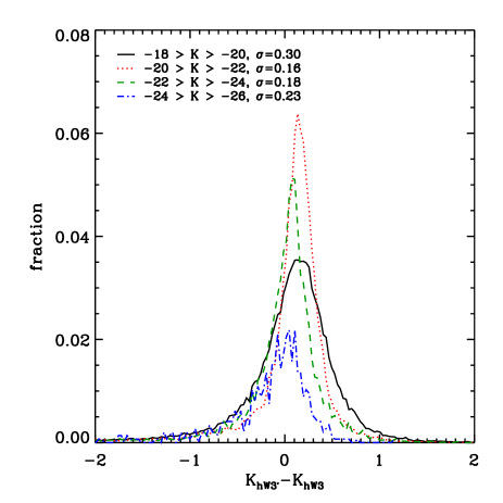
A further comparison of the results of the semi-analytic modelling is presented in Fig. 12. In this plot we show the distribution of K-band magnitude differences, $K_{\tt hW3}-K_{\tt hW3^{\prime}}$, for the central galaxies of “matched” haloes (c.f. §4.2). The predicted properties of galaxies in the WMAP3 cosmology are quite accurately reproduced by our scaled simulations. Typical random differences are below $0.25$ magnitudes over the whole magnitude range and systematic errors are below $0.13$ magnitudes.

5 Conclusions

In this paper we have introduced an algorithm that allows us to scale the output of a cosmological N-body simulation carried out for one specific set of cosmological parameters (for example the WMAP1 parameter set of the Millennium Simulation) so that it faithfully represents the growth of structure in a different cosmology (for example, one with the lower fluctuation amplitude preferred by analyses of the WMAP3 data). Our method builds on the fact that the linear fluctuation amplitude as a function of smoothing scale is sufficient to determine not only the mass function and assembly history of haloes (according to extended Press-Schechter theory) but also the ensemble properties of the large scale structure (in the Zel’dovich approximation). We therefore re-scale the box-size of the simulation and reassign redshifts to the outputs so that the shape of the smoothed linear power spectrum matches that of the target cosmology on the scales which produce resolved dark matter haloes. This scaling and redshift reassignment then imply a rescaling both of particle mass, and of the nonlinear “thermal” velocities in each output. Finally, we use the Zel’dovich approximation to modify the amplitude of the long-wavelength quasilinear modes in order to account for the difference in shape on large scales between the smoothed linear power spectrum of the original cosmology (after scaling) and that of the target cosmology. This modification is effectively a rescaling of the displacements and peculiar velocities produced by each individual long-wavelength (low $\mn@boldsymbol{k}$) mode.

We tested our method by applying it to an N-body simulation based on the WMAP1 parameters to mimic the mass distribution expected in the WMAP3 cosmology. We compared the results with those from a matched N-body simulation run directly in the target cosmology (WMAP3). These two cosmological models span the range of power spectrum shape and amplitude among the models currently considered plausible. Thus we expect our comparison to give conservative estimates of the accuracy of our method.

We found that on large scales the target mass distribution is recovered to high precision ($<1\%$ on scales $k<0.2\,h{\rm Mpc^{-1}}$) in both real and redshift space. On smaller scales the differences increase ( $5\%$) and can be attributed to differences in the halo mass-concentration relation between the true and scaled simulations. These differences are smaller when one considers the clustering of dark matter haloes, – the distribution actually relevant for galaxy clustering. In the latter case, differences are at the subpercent level over the full range of scales we examined. We also tested the algorithm on an object-by-object basis concluding that the position of individual FoF haloes is reproduced to better than $90\,h^{-1}{\rm kpc}$, and their velocities and FoF masses to better than $10\%$.

The dispersion in the matched properties introduces no appreciable effects in the overall clustering statistics of the halo population. Finally for a representative semi-analytic galaxy formation model, the K magnitudes of central galaxies are accurate to $0.25$ magnitudes with a systematic error of $0.13$ magnitudes.

Understanding the connection between galaxy formation and the background cosmological model is an important challenge that cosmologists will face in the near future. A key step towards this is the creation of realistic physically based theoretical models for the galaxy distribution for a wide range of cosmologies. Our method offers a route to this goal. Its relatively small computational cost enables exploration of a multidimensional cosmological parameter space using a suitable N-body simulation of a single cosmology. In this way the task of creating realistic mock galaxy catalogues for all allowed cosmological parameter sets is greatly simplified. It also becomes possible to update existing high-resolution simulations to any favoured cosmological model at a small fraction of the original computational cost. These goals are important not only to understand the physical processes underlying galaxy formation, but also to ensure optimal exploitation of the information encoded in the very large (and expensive) survey datasets that are currently being assembled. Our scheme makes it possible to study how uncertainties in galaxy formation physics will affect our ability to constrain cosmological parameters through analysis of next-generation galaxy surveys.

Acknowlegdments

We would like to thank C. Baugh, S. Cole and M. Schneider for useful comments and a careful reading of this manuscript.

References

- Angulo et al. (2008) Angulo R. E., Baugh C. M., Frenk C. S., Lacey C. G., 2008, MNRAS, 383, 755
- Baugh (2006) Baugh C. M., 2006, Reports of Progress in Physics, 69, 3101
- Baugh et al. (2004) Baugh C. M., et al., 2004, MNRAS, 351, L44
- Berge et al. (2009) Berge J., Amara A., Refregier A., 2009, ArXiv e-prints
- Bullock et al. (2001) Bullock J. S., Dekel A., Kolatt T. S., Kravtsov A. V., Klypin A. A., Porciani C., Primack J. R., 2001, ApJ, 555, 240
- Carbone et al. (2008) Carbone C., Verde L., Matarrese S., 2008, ApJ, 684, L1
- Cole (1997) Cole S., 1997, MNRAS, 286, 38
- Cole et al. (2001) Cole S., Norberg P., Baugh C. M., Frenk C. S., Bland-Hawthorn J., Bridges T., Cannon R., Colless M., Collins C., Couch W., Cross N., Dalton G., De Propris R., Driver S. P., Efstathiou G., Ellis R. S., Glazebrook K., Jackson C., Lahav O., Lewis I., Lumsden S., Maddox S., Madgwick D., Peacock J. A., Peterson B. A., Sutherland W., Taylor K., 2001, MNRAS, 326, 255
- Cole et al. (2005) Cole S., et al., 2005, MNRAS, 362, 505
- Cooray & Sheth (2002) Cooray A., Sheth R., 2002, Phys. Rep., 372, 1
- Croton et al. (2007) Croton D. J., Norberg P., Gaztañaga E., Baugh C. M., 2007, MNRAS, 379, 1562
- Davis et al. (1985) Davis M., Efstathiou G., Frenk C. S., White S. D. M., 1985, ApJ, 292, 371
- De Lucia & Blaizot (2007) De Lucia G., Blaizot J., 2007, MNRAS, 375, 2
- Debono et al. (2009) Debono I., Rassat A., Refregier A., Amara A., Kitching T., 2009, ArXiv e-prints
- Dolag et al. (2004) Dolag K., Bartelmann M., Perrotta F., Baccigalupi C., Moscardini L., Meneghetti M., Tormen G., 2004, A&A, 416, 853
- Eisenstein et al. (2005) Eisenstein D. J., et al., 2005, ApJ, 633, 560
- Gaztanaga et al. (2008) Gaztanaga E., Miquel R., Sanchez E., 2008, arXiv:astro-ph/0808.1921, 808
- Guzzo et al. (2008) Guzzo L., et al., 2008, Nature, 451, 541
- Harker et al. (2007) Harker G., Cole S., Jenkins A., 2007, MNRAS, 382, 1503
- Hoekstra et al. (2006) Hoekstra H., Mellier Y., van Waerbeke L., Semboloni E., Fu L., Hudson M. J., Parker L. C., Tereno I., Benabed K., 2006, ApJ, 647, 116
- Huterer et al. (2006) Huterer D., Takada M., Bernstein G., Jain B., 2006, MNRAS, 366, 101
- Jennings et al. (2009) Jennings E., Baugh C. M., Angulo R. E., Pascoli S., 2009, ArXiv e-prints
- Lewis et al. (2000) Lewis A., Challinor A., Lasenby A., 2000, ApJ, 538, 473
- Manera et al. (2009) Manera M., Sheth R. K., Scoccimarro R., 2009, ArXiv e-prints
- Matarrese & Verde (2008) Matarrese S., Verde L., 2008, ApJ, 677, L77
- Neistein et al. (2009) Neistein E., Maccio’ A. V., Dekel A., 2009, ArXiv e-prints
- Percival & White (2008) Percival W. J., White M., 2008, arXiv:astro-ph/0808.0003, 808
- Press & Schechter (1974) Press W. H., Schechter P., 1974, ApJ, 187, 425
- Ross et al. (2008) Ross A. J., Brunner R. J., Myers A. D., 2008, ApJ, 682, 737
- Sánchez et al. (2006) Sánchez A. G., Baugh C. M., Percival W. J., Peacock J. A., Padilla N. D., Cole S., Frenk C. S., Norberg P., 2006, MNRAS, 366, 189
- Sánchez et al. (2009) Sánchez A. G., Crocce M., Cabré A., Baugh C. M., Gaztañaga E., 2009, MNRAS, 400, 1643
- Seljak (2008) Seljak U., 2008, arXiv:astro-ph/0807.1770, 807
- Spergel et al. (2007) Spergel D. N., Bean R., Doré O., Nolta M. R., Bennett C. L., Dunkley J., Hinshaw G., Jarosik N., Komatsu E., Page L., Peiris H. V., Verde L., Halpern M., Hill R. S., Kogut A., Limon M., Meyer S. S., Odegard N., Tucker G. S., Weiland J. L., Wollack E., Wright E. L., 2007, ApJS, 170, 377
- Spergel et al. (2003) Spergel D. N., Verde L., Peiris H. V., Komatsu E., Nolta M. R., Bennett C. L., Halpern M., Hinshaw G., Jarosik N., Kogut A., Limon M., Meyer S. S., Page L., Tucker G. S., Weiland J. L., Wollack E., Wright E. L., 2003, ApJS, 148, 175
- Springel (2005) Springel V., 2005, MNRAS, 364, 1105
- Springel et al. (2006) Springel V., Frenk C. S., White S. D. M., 2006, Nature, 440, 1137
- Springel et al. (2005) Springel V., White S. D. M., Jenkins A., Frenk C. S., Yoshida N., Gao L., Navarro J., Thacker R., Croton D., Helly J., Peacock J. A., Cole S., Thomas P., Couchman H., Evrard A., Colberg J., Pearce F., 2005, Nature, 435, 629
- Takahashi et al. (2009) Takahashi R., Yoshida N., Takada M., Matsubara T., Sugiyama N., Kayo I., Nishimichi T., Saito S., Taruya A., 2009, ArXiv e-prints
- Tinker et al. (2008) Tinker J., Kravtsov A. V., Klypin A., Abazajian K., Warren M., Yepes G., Gottlöber S., Holz D. E., 2008, ApJ, 688, 709
- Tormen & Bertschinger (1996) Tormen G., Bertschinger E., 1996, ApJ, 472, 14
- Wang et al. (2008) Wang J., De Lucia G., Kitzbichler M. G., White S. D. M., 2008, MNRAS, 384, 1301
- Zel’dovich (1970) Zel’dovich Y. B., 1970, A&A, 5, 84
- Zheng et al. (2002) Zheng Z., Tinker J. L., Weinberg D. H., Berlind A. A., 2002, ApJ, 575, 617
- Zheng & Weinberg (2007) Zheng Z., Weinberg D. H., 2007, ApJ, 659, 1