Signatures of Primordial non-Gaussianities in the Matter Power-Spectrum and Bispectrum:
the Time-RG Approach

Abstract:

We apply the time-renormalization group approach to study the effect of primordial non-Gaussianities in the non-linear evolution of cosmological dark matter density perturbations. This method improves the standard perturbation approach by solving renormalization group-like equations governing the dynamics of gravitational instability. The primordial bispectra constructed from the dark matter density contrast and the velocity fields represent initial conditions for the renormalization group flow. We consider local, equilateral and folded shapes for the initial non-Gaussianity and analyze as well the case in which the non-linear parameter $f_{\rm NL}$ parametrizing the strength of the non-Gaussianity depends on the momenta in Fourier space through a power-law relation, the so-called running non-Gaussianity. For the local model of non-Gaussianity we compare our findings for the power-spectrum with those of recent N-body simulations and find that they accurately fit the N-body data up to wave-numbers $k\sim 0.25\,h$/Mpc at $z=0$. We also present predictions for the (reduced) matter bispectra for the various shapes of non-Gaussianity.

1 Introduction

During the last years, the use of semi-analytic methods to study the Large Scale Structure (LSS) formation via gravitational instability has experienced a renewed interest, motivated mainly by high precision measurements of statistical properties expected in the next generation of galaxy surveys. These methods typically involve resummation or closure prescriptions and need to be compared with numerical simulations to assess their range of validity. Renomalized perturbation theory  [1, 2] is based on suitable resummations of perturbative terms and is expected to work well for the linear and “weakly non-linear” regime. Perturbation theory can be rewritten in a compact way which makes it possible the use of standard tools of quantum field theory, thus allowing a systematic treatment of perturbative terms in terms only of a finite set of basic building blocks, namely, the initial fields, the linear propagator, which describes the linear evolution of the initial fields and an interaction vertex, responsible for the non linear mode coupling of the fields. This leads to the resummation of infinite classes of perturbation theory diagrams. The renormalization group perturbation theory [3] attempts to regulate the relative divergence of one-loop standard perturbation theory (for a review, see [4]) using renormalization group methods. A path-integral formulation of the Vlasov equation has been developed in [5] in terms of the distribution function in the phase space. The lagrangian resummation theory [6] is an extension of the well-developed Lagrangian perturbation theory. Refs. [7] and [8] proposed a formalism based on path-integrals and renormalization group techniques which provides a systematic resummation scheme of cosmological perturbation theory (subsequently, this formalism was extended in Ref. [9] to calculate the non-linear propagator in the presence of non-Gaussian initial conditions of the fields). Finally, in the Time-Renormalization Group (TRG) approach proposed in Ref. [10], the power spectrum, the bispectrum and higher order correlations, are obtained – at any redshift and for any momentum scale – by integrating a system of differential equations. The method is similar to the familiar BBGKY hierarchy. Truncating at the level of the trispectrum, the solution of the equations corresponds to the summation of an infinite class of perturbative corrections. The approach can be seen as a particular formulation of the renormalization group, in which time is the flow parameter. Compared to other resummation frameworks, this scheme is particularly suited to cosmologies other than $\Lambda$CDM and has been recently applied to compute the non-linear spectrum in presence of neutrino masses [11]. A critical look at the various cosmological perturbation theory techniques can be found in [12].

On the other hand, over the last decade a great deal of evidence has been accumulated from the Cosmic Microwave Background (CMB) anisotropy and Large Scale Structure (LSS) spectra that the observed structures originated from seed fluctuations generated during a primordial stage of inflation. While standard single-field models of slow-roll inflation predict that these fluctuations are very close to Gaussian (see [13, 14]), non-standard scenarios allow for a larger level of non-Gaussianity (NG) (see [15] and references therein). A signal is gaussian if the information it carries is completely encoded in the two-point correlation function, all higher connected correlators being zero. Deviations from Gaussianity are therefore encoded, e.g., in the connected three- and four-point correlation functions which are dubbed the bispectrum and the trispectrum, respectively. A phenomenological way of parametrizing the level of NG is to expand the fully non-linear primordial Bardeen gravitational potential $\Phi$ in powers of the linear gravitational potential $\Phi_{\rm L}$

$$\Phi=\Phi_{\rm L}+f_{\rm NL}\left(\Phi_{\rm L}^{2}-\langle\Phi_{\rm L}^{2}\rangle\right)\,.$$ (1)

The dimensionless quantity $f_{\rm NL}$ sets the magnitude of the three-point correlation function [15]. If the process generating the primordial NG is local in space, the parameter $f_{\rm NL}$ in Fourier space is independent of the momenta entering the corresponding correlation functions; if instead the process which generates the primordial cosmological perturbations is non-local in configuration space, like in models of inflation with non-canonical kinetic terms, $f_{\rm NL}$ acquires a dependence on the momenta. It is clear that detecting a significant amount of NG and its shape either from the CMB or from the LSS offers the possibility of opening a window into the dynamics of the universe during the very first stages of its evolution. Non-Gaussianities are particularly relevant in the high-mass end of the power spectrum of perturbations, i.e. on the scale of galaxy clusters, since the effect of non-Gaussian fluctuations becomes especially visible on the tail of the probability distribution. As a result, both the abundance and the clustering properties of very massive halos are sensitive probes of primordial non-Gaussianities [16, 17, 18, 19, 20, 21, 22, 23, 24, 25], and could be detected or significantly constrained by the various planned large-scale galaxy surveys, both ground based (such as DES, PanSTARRS and LSST) and on satellite (such as EUCLID and ADEPT) see, e.g. [26] and [27], [28]. Furthermore, the primordial NG alters the clustering of dark matter (DM) halos inducing a scale-dependent bias on large scales [29, 30, 31, 32] while even for small primordial NG the evolution of perturbations on super-Hubble scales yields extra contributions on smaller scales [33, 28]. The strongest current limits on the strength of local NG set the $f_{\rm NL}$ parameter to be in the range $-4<f_{\rm NL}<80$ at 95% confidence level [34].

In this paper, we implement the TRG approach to investigate the effects imprinted by a primordial NG in the non-linear evolution of cosmological perturbations. In particular, we will compute the DM power spectrum and the (reduced) bispectrum when some primordial initial NG condition is present. In the TRG approach this information is promptly encoded in the RG equations for the power spectrum and the bispectrum. As a consequence, we can easily study the impact of the various shapes of NG. In particular, we consider the local, the equilateral and the folded shapes. As we shall see, our approach is based on a closure assumption, i.e. we solve the RG equations for the power spectrum and the bispectrum, setting the connected $n$-point correlators to zero starting from the four-point correlator, the trispectrum. While this assumption represents a clear limitation of our approach, nevetheless it provides a well-defined and controllable scheme which allows us to quantify in a precise form the theoretical error associated with the method. For the local model of non-Gaussianity we will compare our findings for the power-spectrum with those of recent N-body simulations and find that they accurately fit rather well the N-body data up to wave-numbers $k\sim 0.25\,h$/Mpc. We will also present predictions for the (reduced) matter bispectra for the various shapes of NG.

The paper is organized as follows. In Section 2 we review the time evolution of the correlators governed by Eulerian dynamics and discuss our truncation hypothesis in comparison with other approaches in the literature. In Section 3 we consider the primordial non-Gaussianities compatible with the truncation scheme of this paper and some theoretically motivated models for the primordial bispectrum. In Section 4, we introduce the reduced bispectrum as a relevant tool to study the effects related to the shape of the primordial bispectrum. In Section 5 we present our results for the power-spectrum and a comparison with the results of N-body simulations for “local” NG. We also present several illustrative plots of the reduced bispectrum for each model of NG. In Section 6, we end with our conclusions and discuss future perspectives on this line of work.

2 Dynamics of Gravitational Instability

2.1 Eulerian Dynamics

Our starting point are the hydrodynamic equations in the “single stream” approximation of a self-gravitating fluid made of cold dark matter collisionless particles in an expanding Universe. In terms of the mass-density fluctuation $\delta$, the peculiar velocity ${\bf v}$ of the fluid and the peculiar gravitational potential $\phi$, the dynamics of the system is governed by the system of equations

$$\frac{\partial\delta}{\partial\tau}+\nabla\cdot[(1+\delta){\bf{v}}]=0,{}$$ (2)

$$\frac{\partial{\bf{v}}}{\partial\tau}+{\cal{H}}{\bf{v}}+({\bf{v}}\cdot\nabla){\bf{v}}=-\nabla\phi,{}$$ (3)

$$\nabla^{2}\phi=\frac{3}{2}{\cal{H}}^{2}\Omega_{m}\delta.$$ (4)

The first two equations are the continuity and Euler equations respectively, while the third one is the Poisson equation obeyed by perturbations on sub-horizon scales. Here, $a$ is the scale factor of the background, $\tau=\int dt/a$ is the conformal time, ${\cal{H}}\equiv d\log a/d\tau=aH$ and $\Omega_{m}$ is the matter density parameter. In the following we restrict our discussion to an Einstein-de Sitter model, so we take $\Omega_{m}=1$. As usual, we take the divergence of the Euler equation and define the velocity divergence $\theta=\nabla\cdot{\bf v}$ and Fourier transform. The resulting equations can be written in a compact notation as [1]

$$(\delta_{ab}\partial_{\eta}+\Omega_{ab})\varphi_{b}({\bf k},\eta)=e^{\eta}\gamma_{abc}({\bf k,-p,-q})\varphi_{b}({\bf p},\eta)\varphi_{c}({\bf q},\eta),$$ (5)

where we define the two-component field $\varphi_{a}(a=1,2)$ through

$$\left(\begin{array}[]{c}\varphi_{1}({\bf k},\eta)\\ \varphi_{2}({\bf k},\eta)\end{array}\right)\equiv\exp(-\eta)\left(\begin{array}[]{c}\delta({\bf k},\eta)\\ -\theta({\bf k},\eta)/{\cal H}\end{array}\right),$$ (10)

$e^{\eta}=a/a_{in}$ for an initial scale factor $a_{in}$ conveniently fixed at an early epoch,

$${\bf\Omega}=\left(\begin{array}[]{cc}1&-1\\ -3/2&3/2\end{array}\right)$$ (13)

and $\gamma_{abc}$ is a vertex function which describes the non-linear coupling of the modes and whose only non-vanishing components are

$$\gamma_{121}({\bf p,\,q,\,k})=\frac{1}{2}\delta({\bf p+q+k})\frac{{\bf(q+k)\cdot q}}{q^{2}},$$ (14)

$$\gamma_{222}({\bf p,\,q,\,k})=\frac{1}{2}\delta({\bf p+q+k})\frac{{\bf(q+k)^{2}q\cdot k}}{k^{2}q^{2}},$$ (15)

$$\gamma_{112}({\bf p,\,q,\,k})=\gamma_{121}({\bf p,\,k,\,q}).$$ (16)

Summation (integration) over repeated index (momenta) is understood in Eq. (5).

2.2 Time evolution of the correlators

Following Ref. [10] the time evolution of the field correlators can be obtained directly from iterative application of the equations of motion (5). The result is an infinite tower of coupled differential equations relating the evolution of $n$-point correlators with the $n$ and $(n+1)$-point correlators evaluated at the same time:

$$\partial_{\eta}\,\langle\varphi_{a}\varphi_{b}\rangle = -\Omega_{ac}\langle\varphi_{c}\varphi_{b}\rangle-\Omega_{bc}\langle\varphi_{a}\varphi_{c}\rangle$$

$$+e^{\eta}\gamma_{acd}\langle\varphi_{c}\varphi_{d}\varphi_{b}\rangle+e^{\eta}\gamma_{bcd}\langle\varphi_{a}\varphi_{c}\varphi_{d}\rangle\,,$$

$$\partial_{\eta}\,\langle\varphi_{a}\varphi_{b}\varphi_{c}\rangle = -\Omega_{ad}\langle\varphi_{d}\varphi_{b}\varphi_{c}\rangle-\Omega_{bd}\langle\varphi_{a}\varphi_{d}\varphi_{c}\rangle-\Omega_{cd}\langle\varphi_{a}\varphi_{b}\varphi_{d}\rangle$$

$$+e^{\eta}\gamma_{ade}\langle\varphi_{d}\varphi_{e}\varphi_{b}\varphi_{c}\rangle+e^{\eta}\gamma_{bde}\langle\varphi_{a}\varphi_{d}\varphi_{e}\varphi_{c}\rangle$$

$$+e^{\eta}\gamma_{cde}\langle\varphi_{a}\varphi_{b}\varphi_{d}\varphi_{e}\rangle\,,$$

$$\partial_{\eta}\,\langle\varphi_{a}\varphi_{b}\varphi_{c}\varphi_{d}\rangle = \cdots$$ (17)

$$\cdots$$

Here, we omitted the time and momentum dependence in order to have compact expressions. To solve this system of equations is equivalent to apply the standard perturbation theory approach in which one calculates the n-point correlation functions by summing an infinite series of perturbative corrections depending on the interaction vertex $\gamma$, the red-shift and the initial statistic of the fields. Next, we introduce the following nomenclature for the first correlation functions of the fields

$$\langle\varphi_{a}({\bf k},\eta)\varphi_{b}({\bf q},\eta)\rangle\equiv\delta_{D}({\bf k}+{\bf q})P_{ab}({\bf k},\eta)$$

$$\langle\varphi_{a}({\bf k},\eta)\varphi_{b}({\bf q},\eta)\varphi_{c}({\bf p},\eta)\rangle\equiv\delta_{D}({\bf k}+{\bf q}+{\bf p})B_{abc}({\bf k},\,{\bf q},\,{\bf p};\,\eta)$$

$$\langle\varphi_{a}({\bf k},\eta)\varphi_{b}({\bf q},\eta)\varphi_{c}({\bf p},\eta)\varphi_{d}({\bf r},\eta)\rangle\equiv\delta_{D}({\bf k}+{\bf q})\delta_{D}({\bf p}+{\bf r})P_{ab}({\bf k},\eta)P_{cd}({\bf p},\eta)$$

$$\qquad+\delta_{D}({\bf k}+{\bf p})\delta_{D}({\bf q}+{\bf r})P_{ac}({\bf k},\eta)P_{bd}({\bf q},\eta)+\delta_{D}({\bf k}+{\bf r})\delta_{D}({\bf q}+{\bf p})P_{ad}({\bf k},\eta)P_{bc}({\bf q},\eta)$$

$$\qquad+\delta_{D}({\bf k}+{\bf q}+{\bf p}+{\bf r})T_{abcd}({\bf k},\,{\bf q},\,{\bf p},\,{\bf r};\,\eta),$$

where $P_{ab}$ is the power spectrum (PS) , $B_{abc}$ is the bispectrum (BS), and $T_{abcd}$ is the connected part of the four-point function, the trispectrum. As said before, if we want to calculate the time evolution of the power-spectrum it will involve the time evolution of the bispectrum, which in turn involves the trispectrum and so on, giving us the infinite tower of equations (2.2). This system can be truncated if we neglect the trispectrum $T_{abcd}=0$, letting us with the following system of two equations for the PS and the BS:

$$\partial_{\eta}\,P_{ab}({\bf k}\,,\eta)=-\Omega_{ac}({\bf k}\,,\eta)P_{cb}({\bf k}\,,\eta)-\Omega_{bc}({\bf k}\,,\eta)P_{ac}({\bf k}\,,\eta)$$

$$\qquad\qquad\quad\quad+e^{\eta}\int d^{3}q\,\left[\gamma_{acd}({\bf k},\,{\bf-q},\,{\bf q-k})\,B_{bcd}({\bf k},\,{\bf-q},\,{\bf q-k};\,\eta)\right.$$

$$\qquad\qquad\qquad\qquad\qquad\left.+B_{acd}({\bf k},\,{\bf-q},\,{\bf q-k};\,\eta)\,\gamma_{bcd}({\bf k},\,{\bf-q},\,{\bf q-k})\right]\,,$$

$$\partial_{\eta}\,B_{abc}({\bf k},\,{\bf-q},\,{\bf q-k};\,\eta)=-\Omega_{ad}({\bf k}\,,\eta)B_{dbc}({\bf k},\,{\bf-q},\,{\bf q-k};\,\eta)$$

$$\qquad\qquad\qquad\qquad\qquad\quad-\Omega_{bd}({\bf-q}\,,\eta)B_{adc}({\bf k},\,{\bf-q},\,{\bf q-k};\,\eta)$$

$$\qquad\qquad\qquad\qquad\qquad\quad-\Omega_{cd}({\bf q-k}\,,\eta)B_{abd}({\bf k},\,{\bf-q},\,{\bf q-k};\,\eta)$$

$$\qquad\qquad\qquad\qquad\qquad\quad+2e^{\eta}\left[\gamma_{ade}({\bf k},\,{\bf-q},\,{\bf q-k})P_{db}({\bf q}\,,\eta)P_{ec}({\bf k-q}\,,\eta)\right.$$

$$\qquad\qquad\qquad\qquad\qquad\quad+\gamma_{bde}({\bf-q},\,{\bf q-k},\,{\bf k})P_{dc}({\bf k-q}\,,\eta)P_{ea}({\bf k}\,,\eta)$$

$$\qquad\qquad\qquad\qquad\qquad\quad+\left.\gamma_{cde}({\bf q-k},\,{\bf k},\,{\bf-q})P_{da}({\bf k}\,,\eta)P_{eb}({\bf q}\,,\eta)\right]\,.$$ (18)

The system can be formally solved in the form

$$P_{ab}({\bf k}\,,\eta)=g_{ac}(\eta,0)g_{bd}(\eta,0)P_{cd}({\bf k}\,,\eta=0)$$

$$\qquad\qquad\quad\quad+\int_{0}^{\eta}d\eta^{\prime}e^{\eta^{\prime}}\int d^{3}q\,g_{ae}(\eta,\eta^{\prime})g_{bf}(\eta,\eta^{\prime})$$

$$\qquad\qquad\quad\quad\times\left[\gamma_{ecd}({\bf k},\,{\bf-q},\,{\bf q-k})\,B_{fcd}({\bf k},\,{\bf-q},\,{\bf q-k};\,\eta^{\prime})+(e\longleftrightarrow f)\right]$$

$$B_{abc}({\bf k},\,{\bf-q},\,{\bf q-k};\,\eta)=g_{ad}(\eta,0)g_{be}(\eta,0)g_{cf}(\eta,0)B_{def}({\bf k},\,{\bf-q},\,{\bf q-k};\eta=0)$$

$$\qquad\qquad\qquad\qquad\quad+2\int_{0}^{\eta}d\eta^{\prime}e^{\eta^{\prime}}g_{ad}(\eta,\eta^{\prime})g_{be}(\eta,\eta^{\prime})g_{cf}(\eta,\eta^{\prime})$$

$$\qquad\qquad\qquad\qquad\quad\times\left[\gamma_{dgh}({\bf k},\,{\bf-q},\,{\bf q-k})P_{eg}({\bf q}\,,\eta^{\prime})P_{fh}({\bf k-q}\,,\eta^{\prime})\right.$$

$$\qquad\qquad\qquad\qquad\quad+\gamma_{egh}({\bf-q},\,{\bf q-k},\,{\bf k})P_{fg}({\bf k-q}\,,\eta^{\prime})P_{dh}({\bf k}\,,\eta^{\prime})$$

$$\qquad\qquad\qquad\qquad\quad+\left.\gamma_{fgh}({\bf q-k},\,{\bf k},\,{\bf-q})P_{dg}({\bf k}\,,\eta^{\prime})P_{eh}({\bf q}\,,\eta^{\prime})\right]\,,$$ (19)

where $g_{ac}({\bf k},\eta,\eta^{\prime})$ is the linear propagator which is the Green’s function of the linearized version of equation (5) (by setting $\gamma=0$) and gives the time evolution of the fields at linear order: $\varphi_{a}^{L}({\bf k},\eta)=g_{ac}({\bf k},\eta,\eta^{\prime})\varphi_{c}^{L}({\bf k},\eta^{\prime})$. The subscript $L$ stands for the linear order approximation. From Eq. (2.2) one gets an insight on the effect of our only approximation, namely, the truncation prescription $T_{abcd}=0$. First, the solution for the bispectrum is formally “tree-level”, i.e. it contains no momentum integration. It has the same structure as the lowest perturbative contribution to the bispectrum, but with the linear power spectra replaced by the resummed, time-dependent ones. Inserting the bispectrum in the solution for the power spectrum, we see that it is formally one loop (one momentum integral), but with resummed power spectra in the loops instead of linear ones. In diagrammatic terms, starting from the one loop diagrams for the power spectrum (which have been computed by Taruya et al. [35], for the non-Gaussian case), one is adding all the infinite contributions which can be obtained by adding corrections to the internal power spectra lines at any perturbative order. We use the language of Feynman diagrams introduced in [7, 8, 10] to represent diagrammatically the perturbative contributions to the correlators. The basic building blocks of this diagrammatic approach are shown in figure 1. In terms of them, we can represent the lowest order terms of this procedure as shown in figure 3. On the other hand, the comparison of the bispectrum with the computation by Sefusatti [36] is not so straightforward. Compared to that computation we, again, add the corrections to the power spectra lines at all orders, but we do not include the corrections to the vertex, which Sefusatti computed at one-loop. In order to do that, we should go beyond our truncation approximation and include the trispectrum in the hierarchy of our equations. This can be easily understood if one recalls that in perturbation theory the connected four-point correlator always gets a contribution which is generated by the bispectrum. It is precisely this contribution which generates the one-loop correction to the bispectrum which can be seen as a correction to the interaction vertices $\gamma$. Diagrammatically, the terms included and not included in this approximation are shown in figure 3. Including the trispectrum is straightforward in the TRG approach and we leave this to future work. On general grounds, we expect that the inclusion of the trispectrum will push the length scale where the method works to smaller scales. For a more detailed explanation of the diagrammatic of the method the reader is referred to Sections 3 and 4 in Ref. [10].

Figure 1: Basic building blocks for the perturbative approach with non-gaussian initial conditions. The linear propagator $g_{ab}(\eta_{a},\eta_{b})$ is causally oriented from the time $\eta_{b}$ (dashed segment) to $\eta_{a}$ (solid segment). The interaction vertex $e^{\eta}\gamma_{abc}$ introduces the non linear mode coupling of the fields. The square on the linear power spectrum diagram, represents the initial conditions of the power spectrum, while the triangle in the linear bispectrum diagram represents the initial bispectrum, given by the sum of the newtonian contribution at $z=z_{in}$ and the contribution due to primordial non-Gaussianities.

Figure 2: Diagrammatic representation of the formal solution for PS and BS. The first two lines represents the lowest order contributions to the PS equation. The first line is the ${\cal O}(\gamma^{2})$ contribution to the PS. The second line is the contribution coming from the non-vanishing initial BS which is a tree level, ${\cal O}(\gamma)$, contribution. The the third line is the tree level, ${\cal}O(\gamma)$, contribution to the BS.

Figure 3: Perturbative corrections to ${\cal O}(\gamma^{3})$ order for the bispectrum which are included (left), and not included (right) by implementing the truncation prescription $T_{abcd}=0$.

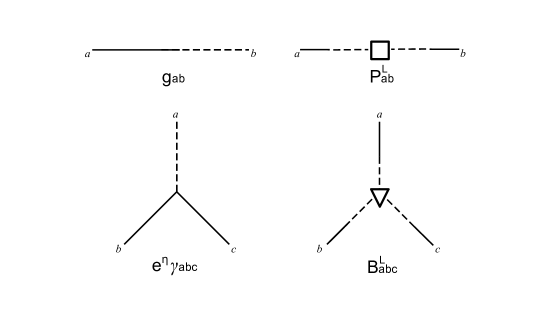
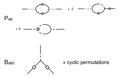
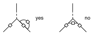
3 Bispectrum Initial Conditions

In this section we calculate the initial conditions, at redshift $z=z_{in}$, for the system (2.2) for our case of non-Gaussian primordial statistics. To this end, we calculate the three-point correlators for the matter density contrast and velocity divergence up to second order terms taking into account the effect imprinted by primordial non-Gaussianities. In other words, we assume that second order perturbation theory holds from $z=\infty$ to $z=z_{in}$, and the resummation embodied by the TRG is active from $z_{in}$ down to $z=0$. We follow the notations and results of Ref. [33] where the effects of primordial non-Gaussianities in the general relativistic cosmological evolution of matter perturbations were calculated up to second order in both the comoving and Poisson gauge, deep in the matter dominated epoch.

Under certain conditions that we shall specify shortly, the results of [33] can be extended to the case of a $\Lambda$CDM cosmology. In this case, the linear order solution of the fields are $\delta^{(1)}_{{\bf k}}(\tau)=D_{+}(a)\delta^{(0)}_{{\bf k}}$ and $\theta^{(1)}_{{\bf k}}(\tau)=-{\cal H}f(\tau)D_{+}(a)\delta^{(0)}_{{\bf k}}$ where $D_{+}(a)$ is the linear growth factor of density perturbations and $f(\tau)=d\ln D_{+}(a)/d\ln a$. Information about the cosmological parameters of the background will be encoded in $D_{+}(a)$ and $f(\tau)$. At this point, being interested in fixing the initial conditions at some early $z_{in}$, we use the approximation $\Omega_{m}/f(\tau)^{2}\approx 1$ which, as discussed in Ref. [4](see also Appendix B of Ref. [37]), is a condition respected during most of the cosmological time evolution. Within this approximation one can simply use the kernels as can be derived from Ref. [33], properly replacing the conformal time $\tau$ in terms of the functions $D_{+}(a)$ and $f(\tau)$. Then, the second order expansions for the matter density perturbation and velocity divergence acquire the form

$$\delta_{{\bf k}}(\tau)=\delta^{(1)}_{{\bf k}}(\tau)+\frac{1}{2}\delta^{(2)}_{{\bf k}}(\tau)=\delta^{(1)}_{{\bf k}}(\tau)+\int d^{3}{\bf k}_{1}d^{3}{\bf k}_{2}\,{\cal K}_{\delta}({\bf k}_{1},{\bf k}_{2};\tau)\delta^{(1)}_{{\bf k}_{1}}(\tau)\delta^{(1)}_{{\bf k}_{2}}(\tau)\delta_{D}({\bf k}_{12}-{\bf k}),$$ (20)

$$\theta_{{\bf k}}(\tau)=\theta^{(1)}_{{\bf k}}(\tau)+\frac{1}{2}\theta^{(2)}_{{\bf k}}(\tau)=\theta^{(1)}_{{\bf k}}(\tau)+\int d^{3}{\bf k}_{1}d^{3}{\bf k}_{2}\,{\cal K}_{\theta}({\bf k}_{1},{\bf k}_{2};\tau)\theta^{(1)}_{{\bf k}_{1}}(\tau)\theta^{(1)}_{{\bf k}_{2}}(\tau)\delta_{D}({\bf k}_{12}-{\bf k}),$$ (21)

where we introduced the notation ${\bf k}_{ij\cdots}={\bf k}_{i}+{\bf k}_{j}+\cdots$ and, following the procedure and the results in [33] we find that

$${\cal K}_{\delta}({\bf k}_{1},{\bf k}_{2};\tau) = {\cal K}_{\delta}^{N}({\bf k}_{1},{\bf k}_{2})+6f_{\rm NL}^{\delta}({\bf k}_{1},{\bf k}_{2})\frac{k^{2}E(\tau)}{k_{1}^{2}k_{2}^{2}},$$ (22)

$${\cal K}_{\theta}({\bf k}_{1},{\bf k}_{2};\tau) = -\frac{1}{{\cal H}f(\tau)}\left[{\cal K}_{\theta}^{N}({\bf k}_{1},{\bf k}_{2})+6f_{\rm NL}^{\theta}({\bf k}_{1},{\bf k}_{2})\frac{k^{2}E(\tau)}{k_{1}^{2}k_{2}^{2}}\right],$$ (23)

where $E(\tau)\equiv H_{0}^{2}\Omega_{m,0}/(4D_{+}(a))$. In the equations (22)-(23)

$${\cal K}_{\delta}^{N}({\bf k}_{1},{\bf k}_{2}) \equiv \frac{5}{7}+\frac{2}{7}\frac{({\bf k}_{1}\cdot{\bf k}_{2})^{2}}{k_{1}^{2}k_{2}^{2}}+\frac{1}{2}\frac{{\bf k}_{1}\cdot{\bf k}_{2}\left(k_{1}^{2}+k_{2}^{2}\right)}{k_{1}^{2}k_{2}^{2}}$$ (24)

$${\cal K}_{\theta}^{N}({\bf k}_{1},{\bf k}_{2}) \equiv \frac{3}{7}+\frac{4}{7}\frac{({\bf k}_{1}\cdot{\bf k}_{2})^{2}}{k_{1}^{2}k_{2}^{2}}+\frac{1}{2}\frac{{\bf k}_{1}\cdot{\bf k}_{2}\left(k_{1}^{2}+k_{2}^{2}\right)}{k_{1}^{2}k_{2}^{2}}$$ (25)

are the standard one-loop Newtonian kernels for the expansion of the fields [38], and

$$f_{\rm NL}^{\delta}({\bf k}_{1},{\bf k}_{2}) = \frac{5}{3}(a_{\rm NL}-1)+{\cal O}(1)$$ (26)

$$f_{\rm NL}^{\theta}({\bf k}_{1},{\bf k}_{2}) = \frac{5}{3}(a_{\rm NL}-1)+{\cal O}(1)$$ (27)

are the terms arising from non-Gaussian initial statistics. Here $a_{\rm NL}$ parametrizes the primordial NG level, according to the notations of Ref. [33]. The ${\cal O}(1)$ terms in Eqs. (26)-(27) depend on the Fourier-space configuration. These terms represent general relativistic horizon-scale corrections [33] and have proven to be relevant in the description of the clustering of halos in the presence of non-Gaussian initial conditions as was recently discussed in [28]. Nevertheless, for our purposes here, we will deal with the primordial NG in the limit $|a_{\rm NL}-1|\gg 1$, so, these terms become irrelevant and we will keep just the constant part of the non-Gaussian terms $f^{\delta,\theta}_{\rm NL}\simeq 5(a_{\rm NL}-1)/3$.
We assume that primordial NG is encoded in the curvature perturbations described through the Bardeen’s gauge invariant potential $\Phi$ which, on sub-horizon scales reduces to the peculiar gravitational potential $\phi$ up to a minus sign. The second order expansion of the matter density and velocity divergence can be expressed in terms of $\Phi$, obtaining

$$\delta_{{\bf k}}(\tau) = {\cal M}(k,a)\Phi({\bf k})$$ (28)

$$+ \int d^{3}{\bf k}_{1}d^{3}{\bf k}_{2}\,{\cal K}_{\delta}^{N}({\bf k}_{1},{\bf k}_{2}){\cal M}(k_{1},a)\Phi^{(1)}_{{\bf k}_{1}}{\cal M}(k_{2},a)\Phi^{(1)}_{{\bf k}_{2}}\delta_{D}({\bf k}_{12}-{\bf k})$$

$$-\frac{\theta_{{\bf k}}(\tau)}{{\cal H}f} = {\cal M}(k,a)\Phi({\bf k})$$ (29)

$$+ \int d^{3}{\bf k}_{1}d^{3}{\bf k}_{2}\,{\cal K}_{\theta}^{N}({\bf k}_{1},{\bf k}_{2}){\cal M}(k_{1},a)\Phi^{(1)}_{{\bf k}_{1}}{\cal M}(k_{2},a)\Phi^{(1)}_{{\bf k}_{2}}\delta_{D}({\bf k}_{12}-{\bf k})\,,$$

where the primordial gravitational potential $\Phi$ includes the linear part and the contributions coming from primordial non-Gaussianities. The function ${\cal M}$ comes from the Poisson equation

$${\cal M}(k,a)=\frac{2k^{2}T(k)}{3\Omega_{m,0}{H}_{0}^{2}}D_{+}(a),$$ (30)

with $T(k)$ being the transfer function of matter fluctuations normalized such that $T(k)\rightarrow 1$ when $k\rightarrow 0$. The expressions above account for a generic shape of the primordial NG, and also for a $\Lambda$CDM universe. Notice that, while for the primordial gravitational potential, the first lines of Eq. (28) and (29) are exact, over the second lines applies the same approximations that led to eqs. (20)-(21). Using the expressions above, and recalling the definition (10) in which we replace $\varphi_{2}\rightarrow\varphi_{2}/f(\tau)$ in the $\Lambda$CDM case, the initial BS components can be written as

$$\left\langle\varphi_{1}({\bf k}_{1})\varphi_{1}({\bf k}_{2})\varphi_{1}({\bf k}_{3})\right\rangle = e^{-3\eta}\delta_{D}({\bf k}_{1}+{\bf k}_{2}+{\bf k}_{3})\times$$ (31)

$$\left[2{\cal K}_{\delta}^{N}({\bf k}_{1},{\bf k}_{2}){\cal M}^{2}(k_{1},a){\cal M}^{2}(k_{2},a)P_{\Phi}(k_{1})P_{\Phi}(k_{2})+cycl.\right]$$

$$+ e^{-3\eta}{\cal M}(k_{1},a){\cal M}(k_{2},a){\cal M}(k_{3},a)\left\langle\Phi_{p}({\bf k}_{1})\Phi_{p}({\bf k}_{2})\Phi_{p}({\bf k}_{3})\right\rangle$$

$$\left\langle\varphi_{2}({\bf k}_{1})\varphi_{2}({\bf k}_{2})\varphi_{2}({\bf k}_{3})\right\rangle = e^{-3\eta}\delta_{D}({\bf k}_{1}+{\bf k}_{2}+{\bf k}_{3})\times$$ (32)

$$\left[2{\cal K}_{\theta}^{N}({\bf k}_{1},{\bf k}_{2}){\cal M}^{2}(k_{1},a){\cal M}^{2}(k_{2},a)P_{\Phi}(k_{1})P_{\Phi}(k_{2})+cycl.\right]$$

$$+ e^{-3\eta}{\cal M}(k_{1},a){\cal M}(k_{2},a){\cal M}(k_{3},a)\left\langle\Phi_{p}({\bf k}_{1})\Phi_{p}({\bf k}_{2})\Phi_{p}({\bf k}_{3})\right\rangle$$

$$\left\langle\varphi_{1}({\bf k}_{1})\varphi_{2}({\bf k}_{2})\varphi_{2}({\bf k}_{3})\right\rangle = 2e^{-3\eta}\delta_{D}({\bf k}_{1}+{\bf k}_{2}+{\bf k}_{3})\times$$ (33)

$$\left[{\cal K}_{\theta}^{N}({\bf k}_{1},{\bf k}_{2}){\cal M}^{2}(k_{1},a){\cal M}^{2}(k_{2},a)P_{\Phi}(k_{1})P_{\Phi}(k_{2})\right.$$

$$+ \left.{\cal K}_{\theta}^{N}({\bf k}_{1},{\bf k}_{3}){\cal M}^{2}(k_{1},a){\cal M}^{2}(k_{3},a)P_{\Phi}(k_{1})P_{\Phi}(k_{3})\right.$$

$$+ \left.{\cal K}_{\delta}^{N}({\bf k}_{2},{\bf k}_{3}){\cal M}^{2}(k_{2},a){\cal M}^{2}(k_{3},a)P_{\Phi}(k_{2})P_{\Phi}(k_{3})\right]$$

$$+ e^{-3\eta}{\cal M}(k_{1},a){\cal M}(k_{2},a){\cal M}(k_{3},a)\left\langle\Phi_{p}({\bf k}_{1})\Phi_{p}({\bf k}_{2})\Phi_{p}({\bf k}_{3})\right\rangle$$

$$\left\langle\varphi_{1}({\bf k}_{1})\varphi_{1}({\bf k}_{2})\varphi_{2}({\bf k}_{3})\right\rangle = 2e^{-3\eta}\delta_{D}({\bf k}_{1}+{\bf k}_{2}+{\bf k}_{3})\times$$ (34)

$$\left[{\cal K}_{\theta}^{N}({\bf k}_{1},{\bf k}_{2}){\cal M}^{2}(k_{1},a){\cal M}^{2}(k_{2},a)P_{\Phi}(k_{1})P_{\Phi}(k_{2})\right.$$

$$+ \left.{\cal K}_{\delta}^{N}({\bf k}_{1},{\bf k}_{3}){\cal M}^{2}(k_{1},a){\cal M}^{2}(k_{3},a)P_{\Phi}(k_{1})P_{\Phi}(k_{3})\right.$$

$$+ \left.{\cal K}_{\delta}^{N}({\bf k}_{2},{\bf k}_{3}){\cal M}^{2}(k_{2},a){\cal M}^{2}(k_{3},a)P_{\Phi}(k_{2})P_{\Phi}(k_{3})\right]$$

$$+ e^{-3\eta}{\cal M}(k_{1},a){\cal M}(k_{2},a){\cal M}(k_{3},a)\left\langle\Phi_{p}({\bf k}_{1})\Phi_{p}({\bf k}_{2})\Phi_{p}({\bf k}_{3})\right\rangle$$

where $P_{\Phi}(k)$ is the gravitational potential power-spectrum, see Eq. (39) below. The expressions above constitute the initial conditions for the bispectrum in the system (2.2) and must be evaluated at the initial time, for which $\eta=\log{a}/{a_{in}}=0$. Notice that the expressions above are separated in a perturbative Newtonian term, which is the first term on the r.h.s of each equation, and in a primordial part, which is the term including the three-point correlator of the primordial gravitational potential.

3.1 Primordial NG: Shapes and Running

The functional form of the bispectrum of the primordial gravitational potential entering in Eqs. (31)-(34).

$$\langle\Phi({\bf k}_{1})\Phi({\bf k}_{2})\Phi({\bf k}_{3})\rangle=\delta_{D}({\bf k}_{1}+{\bf k}_{2}+{\bf k}_{3})B_{\Phi}(k_{1},k_{2},k_{3})$$ (35)

depends on the details of the mechanism that generated the primordial fluctuations. In the following we will analyze three representative phenomenological models associated to different mechanisms generating the primordial NG. Note that there exist other possible configurations (see for instance [41]) which correspond to more general deviations from the standard slow-roll inflation and which are not well described by the models treated here.

3.1.1 Local Shape

In the local model, the NG for Bardeen’s gauge invariant primordial gravitational potential $\Phi$ is generated by a quadratic expansion which is local in real space

$$\Phi({\bf x})=\Phi_{\rm L}({\bf x})+f_{\rm NL}^{\rm local}(\Phi_{\rm L}^{2}({\bf x})-\langle\Phi_{\rm L}^{2}\rangle)\;,$$ (36)

where $\Phi_{L}$ is the linear Gaussian part of the potential. The dimensionless constant $f_{\rm NL}$ defines the NG strength in this model. One must also notice that, since $\Phi$ and $\Phi_{L}$ evolve proportionally to $g(a)=D_{+}(a)/a$, the Eq. (36), and consequently, the definition of $f_{\rm NL}$, depends on the choice of the redshift at which this equation is extrapolated. The relation between two extrapolation choices $a$ and $b$ is expressed through $f_{\rm NL}^{a}=g(z=z_{b})/g(z=z_{a})f_{\rm NL}^{b}$. Two common conventions in the literature are the LSS convention in which Eq. (36) is extrapolated to $z=0$, and the CMB convention which extrapolates to $z=\infty$. They are related through $f_{\rm NL}^{\rm LSS}=g(z=\infty)/g(0)f_{\rm NL}^{\rm CMB}$ where $g(z=\infty)/g(0)\simeq 1.3064$. In this paper, we assume the CMB convention, which implies that $\Phi$ is evaluated deep in the matter era. From equation (36) one can easily derive the expression for the local bispectrum

$$B_{\Phi}(k_{1},k_{2},k_{3})=f_{\rm NL}^{\rm local}F^{\rm local}(k_{1},k_{2},k_{3}),$$ (37)

where

$$F^{\rm local}(k_{1},k_{2},k_{3}) = 2\left[P_{\Phi}(k_{1})P_{\Phi}(k_{2})+P_{\Phi}(k_{1})P_{\Phi}(k_{3})+P_{\Phi}(k_{2})P_{\Phi}(k_{3})\right]$$

$$= 2\Delta_{\Phi}^{2}\cdot\left(\frac{1}{(k_{1}k_{2})^{3-(n_{s}-1)}}+\frac{1}{(k_{1}k_{3})^{3-(n_{s}-1)}}+\frac{1}{(k_{2}k_{3})^{3-(n_{s}-1)}}\right)$$

and $P_{\Phi}(k)$ is the gravitational potential power spectrum

$$\langle\Phi({\bf k}_{1})\Phi({\bf k}_{2})\rangle\equiv\delta^{3}\big{(}{\bf k}_{12}\big{)}P_{\Phi}(k_{1})=\delta^{3}\big{(}{\bf k}_{12}\big{)}\Delta_{\Phi}\cdot k^{-3+(n_{s}-1)}$$ (39)

with scalar amplitude $\Delta_{\Phi}$ and tilt $n_{s}$. In slow-roll single scalar field inflation, $f_{\rm NL}^{\rm local}$ is suppressed by the slow-roll parameters and consequently the primordial NG is unmeasurably small [13, 14]. However, in the presence of light fields other than the inflaton, as for instance in the curvaton model or in multi-field models, inflation can produce large NG of the local type with $|f_{\rm NL}^{\rm local}|\sim{\cal O}(10^{2})$ [15]. The strongest current limits on the strength of local NG set the $f^{\rm loc}_{\rm NL}$ parameter to be in the range $-4<f^{\rm loc}_{\rm NL}<80$ at 95% confidence level [34].

3.1.2 Equilateral Shape

We can also consider inflationary models with higher order derivative operators and non canonical kinetic terms, such as the DBI model [44], for instance. In this case, as was discussed in [45], the primordial bispectrum is well described by the equilateral template $B_{\Phi}(k_{1},k_{2},k_{3})=f_{\rm NL}^{\rm eq}F^{\rm eq}(k_{1},k_{2},k_{3})$, where

$$F^{\rm eq}(k_{1},k_{2},k_{3}) = 6\left(-P_{\Phi}(k_{1})P_{\Phi}(k_{2})+(2\;{\rm perm}.)-2\left\{P_{\Phi}(k_{1})P_{\Phi}(k_{2})P_{\Phi}(k_{3})\right\}^{2/3}\right.$$ (40)

$$\left.+\left(P_{\Phi}(k_{1})\left\{P_{\Phi}(k_{2})\right\}^{2}\left\{P_{\Phi}(k_{3})\right\}^{3}\right)^{1/3}+(5\;{\rm perm}.)\right)$$

$$= 6\Delta_{\Phi}^{2}\cdot\left(-\frac{1}{(k_{1}k_{2})^{3-(n_{s}-1)}}-(2\;{\rm perm}.)-\frac{2}{(k_{1}k_{2}k_{3})^{2-\frac{2}{3}(n_{s}-1)}}\right.$$

$$\left.+\frac{1}{k_{1}^{1-\frac{1}{3}(n_{s}-1)}k_{2}^{2-\frac{2}{3}(n_{s}-1)}k_{3}^{3-(n_{s}-1)}}+(5\;{\rm perm}.)\right)\;.$$

The primordial bispectrum is maximized by configurations with modes of similar momentum scales $k_{1}\approx k_{2}\approx k_{3}$, i.e. for equilateral configurations. At present $f_{\rm NL}^{\rm eq}$ is constrained to be $-125<f_{\rm NL}^{\rm eq}<435$ ($95\%$ C.L.) [34]

3.1.3 Folded Shape

A third template is the so called folded or flattened model. This model is related to the non-Gaussianities generated by deviations coming from the choice of a non-standard adiabatic Bunch-Davies vacuum state as initial state [46, 47]. The associated primordial bispectrum assumes a complicated functional form in terms of the momenta $k_{i}$. Nevertheless, in Ref. [48] it is proposed a factorized template which reflects very well the main features of the primordial NG associated to the choice of a non standard vacuum. The proposed factorized template is $B_{\Phi}(k_{1},k_{2},k_{3})=f_{\rm NL}^{\rm fol.}F^{\rm fol.}(k_{1},k_{2},k_{3})$, with

$$F^{\rm fol.}(k_{1},k_{2},k_{3}) = 6\left(P_{\Phi}(k_{1})P_{\Phi}(k_{2})+(2\;{\rm perm}.)+3\left\{P_{\Phi}(k_{1})P_{\Phi}(k_{2})P_{\Phi}(k_{3})\right\}^{2/3}\right.$$ (41)

$$\left.-\left(P_{\Phi}(k_{1})\left\{P_{\Phi}(k_{2})\right\}^{2}\left\{P_{\Phi}(k_{3})\right\}^{3}\right)^{1/3}+(5\;{\rm perm}.)\right)$$

$$= 6\Delta_{\Phi}^{2}\cdot\left(\frac{1}{(k_{1}k_{2})^{3-(n_{s}-1)}}+(2\;{\rm perm}.)+\frac{3}{(k_{1}k_{2}k_{3})^{2-\frac{2}{3}(n_{s}-1)}}\right.$$

$$\left.-\frac{1}{k_{1}^{1-\frac{1}{3}(n_{s}-1)}k_{2}^{2-\frac{2}{3}(n_{s}-1)}k_{3}^{3-(n_{s}-1)}}-(5\;{\rm perm}.)\right)\;.$$

The primordial bispectrum for this model is maximized by configurations with modes obeying the momentum configuration $k_{2}\approx k_{3}\approx k_{1}/2$. The triangle configurations relevant for each model of NG are represented in figure 4.

Figure 4: Momentum triangle configurations which maximize the templates functions $F(k_{1},k_{2},k_{3})$. (1) The squeezed configuration $k_{3}\ll k_{1}\approx k_{2}$ maximize the template function $F^{\rm local}(k_{1},k_{2},k_{3})$ produced in local models of inflation. (2) The equilateral configuration $k_{1}\approx k_{2}\approx k_{3}$ maximize $F^{\rm eq}(k_{1},k_{2},k_{3})$ which arises on models with higher-order derivatives and non canonical terms. (3) The “folded” or “flattened” configuration $k_{2}\approx k_{3}\approx k_{1}/2$ maximize the $F^{\rm fol.}(k_{1},k_{2},k_{3})$ which is related to the choice of a non-standard vacuum other than the Bunch-Davies vacuum.

3.1.4 Running $f_{\rm NL}$

So far, we have considered a scale independent $f_{\rm NL}$ parameter regardless the shape of the primordial bispectrum. However, recently, several inflationary scenarios have been considered which naturally allow for NG with a generic scale dependence on $f_{\rm NL}$. More specifically, it was shown in Refs. [46] and [49] that single scalar field models of inflation with variable speed of sound $c_{s}$, predict in general a primordial bispectrum of the equilateral type with a scale dependent $f_{\rm NL}$. In the following, for non-Gaussianities of the equilateral type, we adopt the functional form for the scale dependence proposed in [50]:

$$f_{\rm NL}(k_{1},k_{2},k_{3})=f_{{\rm NL},P}\left(\frac{k_{1}+k_{2}+k_{3}}{3k_{P}}\right)^{-2\kappa},$$ (42)

where $f_{{\rm NL},P}$ is the non linear parameter evaluated at some pivot scale $k_{P}$ and $\kappa$ is a free parameter (related to the speed of sound) that quantifies the running on the scale and which is constant at least between CMB and cluster scales [50]. To be consistent with observational constraints, the scale dependence must be very mild, then $|\kappa|\ll 1$. Also, in an interesting discussion regarding the scale dependence of the biasing parameters for the equilateral model, in Ref. [35], the authors found the constraint $|\kappa|\lesssim 0.3$ in order to guarantee the convergence of the integrals quantifying the scale dependence of the biasing. In this paper we thus consider values of the running parameter within $|\kappa|\leq 0.3$. Moreover, we use negatives values of $\kappa$ since in this case the NG is enhanced for scales beyond the pivot scale [50]. Another proposal for the functional dependence on the running $f_{\rm NL}$ was discussed recently in [51]

$$\bar{f}_{\rm NL}(k_{1},k_{2},k_{3})=f_{{\rm NL},P}\left(\frac{(k_{1}k_{2}k_{3})^{1/3}}{k_{P}}\right)^{-2\kappa},$$ (43)

which replaces the arithmetic mean of the momenta in equation (42) with their geometric mean. Notice that the two functions coincide for equilateral configurations. While the last proposal has the virtue of being separable, which simplifies significantly the numerical implementation of the CMB estimator, the equation (42) provides a more accurate description of the primordial bispectrum in DBI models. The functional dependence (43) seems to be better suited for NG of the local type. It was shown recently that non-Gaussianities of the local type exhibit significant scale dependence of the amplitude of the primordial bispectrum [52, 53]. The form of this amplitude depends on the specific details of the underlying inflationary model. For example in the case of standard single-field models of inflation it coincides with the functional form (43) in the equilateral limit. Away from this limit, it is not possible to factor out the geometric mean of the momenta in $f_{\rm NL}$ but, in principle, the essentials of the local model can be roughly captured with the expression (43).

4 Results

For our analysis, we assume cosmological parameters corresponding to a $\Lambda$-CDM model in agreement with the WMAP 5-year data [42]. The cosmological parameters for this model are summarized in Table 1. As discussed before, we use second order perturbation theory from $z=\infty$ to $z=z_{in}$, and the TRG from $z_{in}$ to $z=0$. To get the numerical results presented in the following, we set $z_{in}=50$, and used the CAMB code [43] to derive the linear power-spectrum. In order to reproduce the cosmological model in table 1, we must fix the scalar amplitude to be $\Delta^{2}_{\cal R}=2.48\times 10^{-9}$ in the notations of Ref. [42]. With these parameters we are able to compare our results for the matter power spectrum with the results of N-body simulation of cosmological structure formation with non-Gaussian initial conditions of the local type from Refs. [54] and [55] (see also [56, 29, 57, 58] for N-body simulations with local-type non-Gaussian initial conditions).

We also compute the reduced bispectrum for matter density perturbations. Here we point out some general features about the effect of the primordial non-Gaussianities on the bispectrum based on our results.

Table 1: $\Lambda$-CDM cosmological parameters assumed on this paper.

Model	$h$	$\sigma_{8}$	$n_{s}$	$\Omega_{m}$	$\Omega_{\Lambda}$	$\Omega_{b}$
$\Lambda$-CDM WMAP5	0.701	0.817	0.96	0.279	0.721	0.0462

4.1 The Power Spectrum

Here, we present the results of the power spectrum of the matter density perturbations resulting from the integration of the system (2.2) on the scales of interest for next generation galaxy surveys. In order to evaluate the impact of primordial non-Gaussianities on the power-spectrum we plot the ratio of the power spectra for non-Gaussian and Gaussian initial conditions for different values of the $f_{\rm NL}$ parameter. It must be noticed that the power spectra for both Gaussian and non-Gaussian initial conditions were calculated using the TRG method.

4.1.1 Local Model

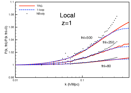
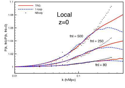
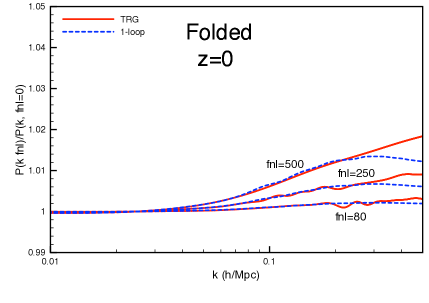
For the local non-Gaussian model, the result of this evaluation is shown in figure 5. For this type of NG we can compare our findings with the results of N-body simulations in [54]. In the figures we also show the result from one-loop perturbation theory, see for instance [35]. We notice that up to $k\sim 0.2\,h$/Mpc, the one-loop and the TRG describes the data very accurately while, for larger values of $k$ we begin to have departures from the data. The difference between one-loop and TRG prediction becomes noticeable for large $f_{\rm NL}$ and for higher wavenumbers and lower redshifts as evidenced in the right panel of Figure 5, which is the result of the evaluation at $z=0$. From the figures we can also infer that the TRG approach allows a less suppressed non-linear growth of the power spectrum in the region $k\gtrsim 0.25\,h$/Mpc. This tendency seems to be general for the different models of primordial NG. The oscillatory behaviour exhibited in the TRG plots are the result of numerical errors in the numerical integration of the system 2.2.

Figure 5: Ratio of the non-Gaussian to Gaussian power spectrum for several values of $f_{\rm NL}$ in the local model. The dots correspond to the data from the N-body simulations of [54]. The red (continuous) line is the TRG result of this paper and the blue (dashed) line is the one-loop result.

4.1.2 Equilateral and Folded Shapes

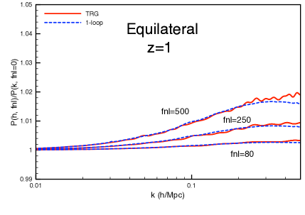
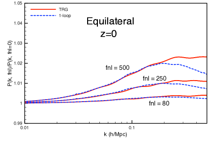
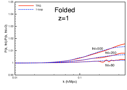
Here, we show the results of the power spectra ratio for equilateral and folded non-Gaussian shapes. The result of this evaluation is shown in Figures 6. Since at present there are no simulations using this type of primordial NG, the results displayed here have a predictive character. Again, as we observed in the local case, when we compare with the one-loop calculation the TRG predictions allow for less suppressed effects of non-Gaussianities, The difference is more evident for scales smaller than $k\sim 0.2\,h$/Mpc and for lower redshifts.

Figure 6: Ratio of the non-Gaussian to Gaussian power spectrum for several values of $f_{\rm NL}$ in the equilateral (top panels) and folded (bottom panels) models. The red (continuous) lines are the TRG result of this paper and the blue (dashed) lines are the one-loop result.

4.1.3 Running $f_{\rm NL}$, equilateral model

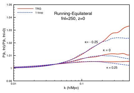
In Figure 7 we plot the power spectrum ratio for the equilateral model with scale dependent $f^{\rm eq}_{\rm NL}$ according to Eq. (42). We choose the pivot scale $k_{P}=0.04\,h$/Mpc, and $\kappa=0,0.25,-0.25$. We see that for positive $\kappa$ we have a suppression in the power spectrum, while, for negative $\kappa$ we can get a significant enhancement of the power spectrum. Notice that the scale dependence of $f^{\rm eq}_{\rm NL}$ can make the effects of primordial NG in the power spectrum of the same order of the local case.

Figure 7: Ratio of the non-Gaussian to Gaussian power spectrum for $f_{\rm NL}=250$ in the equilateral model for different values of $\kappa$. The red (continuous) lines are the TRG result of this paper and the blue (dashed) lines are the one-loop result.

5 The Reduced Bispectrum

As we will be mainly interested in the study of the dependence of the bispectrum on the shape of the momentum triangle, it is convenient to focus the analysis on the reduced bispectrum which is a useful quantity defined as

$$Q(k_{1},k_{2},k_{3})\equiv\frac{B(k_{1},k_{2},k_{3})}{\Sigma(k_{1},k_{2},k_{3})},$$ (44)

where $\Sigma(k_{1},k_{2},k_{3})=P(k_{1})P(k_{2})+P(k_{1})P(k_{3})+P(k_{2})P(k_{3})$. The greatest challenge in the interpretation of galaxy clustering data from any surveys is galaxy bias. As thoroughlly discussed in Ref. [26], the reduced bispectrum provides an excellent determination of linear and non-linear bias parameters of intermediate and high-redhift galaxies, when all measurable triangle configurations down to mildly non-linear scales are included. The reduced bispectrum is also a powerful probe of primordial NG. The planned galaxy surveys at redshift $z>2$ should yield constraints on NG that are comparable to, or even better than, those from CMB experiments. The precise computation of the reduced bispectrum is therefore of primary importance.

Due to statistical homogeneity and isotropy, the bispectrum and the reduced bispectrum depends on time, on the magnitude of two of the momenta, for instance, $k_{1}$ and $k_{2}$, and the angle between them $\cos\theta=\hat{k}_{1}\cdot\hat{k}_{2}$. Figure 4 shows the geometric parameters in the three configurations that we consider in this paper. For gaussian initial conditions and an equilateral configuration, $Q(k,k,k)\simeq 0.57$ at the tree-level in perturbation theory and is independent of scales. On the other hand, $Q(k,k,k)$ exibits a clear scale dependence when some NG is present. The same is true when one departs from the equilateral configuration which reflects the anisotropy on the growth of structures dictated by the non linear Eulerian dynamics. As the NG appears in our RG equations as post-Newtonian term and therefore suppressed at small scales and late times compared to the leading Newtonian terms, it is expected that the NG will be more easily testable at high redshifts and on large scales. This is particularly true for the local shape as the reduced bispectrum (at the tree-level) which is directly proportional to $f_{\rm NL}^{\rm loc}$ scales like $1/{\cal M}(k,a)$.

In our analysis we fix the ratio $k_{2}/k_{1}=2$ and evaluate for different values of $k_{1}$, $f_{\rm NL}$ and for different redshifts. As an extreme case, we also consider the ratio $k_{2}/k_{1}=1$ to have some indications of the maximization of the non-Gaussian effects in the squeezed limit.

5.1 Local model

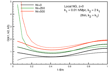
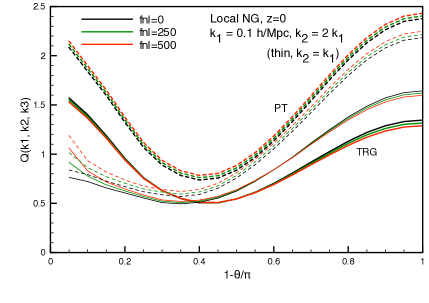
The results of our evaluations for the local model of primordial NG can be seen in Figure 8. From the upper panels in Figure 8, which corresponds to $k=0.01\,h$/Mpc, we see that $Q$ is much more sensitive to the effect of the primordial NG for small $k_{1}$. In this case we see that the effect of non-Gaussianities on $Q$ is almost independent of $\theta$ for $z=1$ and $z=0$. Nevertheless, for higher redshifts we can see clearly a maximization in the effect of the non Gaussianities in the squeezed limit which corresponds to $\theta\rightarrow\pi$. The effect is dramatically maximized when we consider the squeezed limit of the configuration $k_{2}/k_{1}=1$ as shown by the thin lines of this Figure. In this configuration, the condition $\theta\rightarrow\pi$ is equivalent to $k_{3}/k_{1}\ll 1$. We can understand the behaviour at this limit by studying the first terms in the perturbative expansion of $Q$. The first term containing the non-Gaussian contributions is $Q^{(0),\,\rm{NG}}(k_{1},k_{2},k_{3})\equiv B^{(0),\,\rm{NG}}(k_{1},k_{2},k_{3})/\Sigma^{0}(k_{1},k_{2},k_{3})$. Going to the squeezed limit $k_{3}/k_{1}\ll 1$, this non-Gaussian contribution scales roughly as $Q^{(0),\,\rm{NG}}(k_{1},k_{1},k_{3})\sim f_{\rm NL}/k_{3}^{2}$. This is why in the limit $\theta\rightarrow\pi$, the non-Gaussian component is huge, actually, it is divergent. For this reason we should not consider the evaluation at this extreme configuration as a precise prediction but as an indication of the behaviour at this limit. The exact scaling of $Q^{(0),\,\rm{NG}}$ depends also on the precise details of the transfer function which could alleviate up to some extent the divergent behaviour in this configuration for higher values of $k_{1}$ as suggested by the results in the lower panels of Figure 8. On the other hand, the tree level Gaussian component of the reduced bispectrum $Q^{(0)}(k_{1},k_{2},k_{3})\equiv B^{tree}(k_{1},k_{2},k_{3})/\Sigma^{0}(k_{1},k_{2},k_{3})$, where $B^{tree}(k_{1},k_{2},k_{3})$ is the Newtonian piece of the bispectrum, scales like $Q^{(0)}(k_{1},k_{1},k_{3})\sim k_{3}/k_{1}$ in the squeezed limit and consequently it goes to zero for $\theta\rightarrow\pi$. This tendency can be seen in the black-thin lines in the upper panels of Figure 8. Finally, the impact of non Gaussianities for higher values of $k_{1}$ is much smaller and is almost independent of $f_{\rm NL}$ as can be seen in the bottom panel of Figure 8 which corresponds to $k=0.1\,h$/Mpc.

Figure 8: The reduced bispectrum for the local model of NG with fixed $k_{1}$ and ratio $k_{2}/k_{1}=2$ (thick lines) and $k_{2}/k_{1}=1$ (thin lines). The left panels shows the evaluation at $z=1$ while the right panels does it for $z=0$. In each case we plot $Q$ for non-Gaussian initial conditions with $f_{\rm NL}=250$ (green-dotted) and $f_{\rm NL}=500$ (red-dashed). From top to bottom we plot $Q$ for $k=0.01,\,0.05,$ and $0.1\,h$/Mpc respectively. The thin red-dashed and green-dotted lines in the upper panel show the divergent behaviour due to the non-Gaussian component near $\theta=\pi$ in the squeezed limit. The black-continuous thin line on the same panels represent the Gaussian component of the reduced bispectrum which approaches to zero as $\theta\rightarrow\pi$ in this configuration.

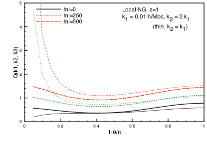
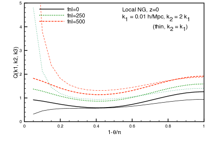
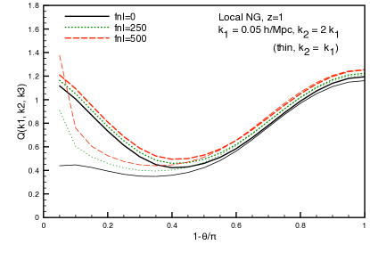
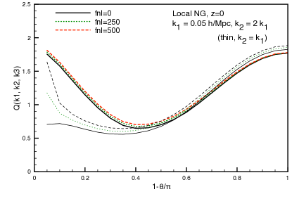
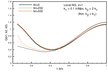
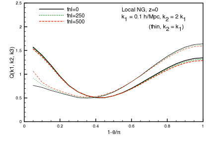
Figure 9 shows the comparison of the TRG evaluation with the perturbation theory (PT) tree level reduced bispectrum $Q^{(0)}$ for several values the $f_{\rm NL}$ at redshift $z=0$. These plots are meant to help understanding the relevance of non linear effects at different scales and redshifts. It is noticeable that there is a remarkable change in the impact of non linear effects depending on the scales we are considering. For instance, in the left panel of figure 9, we plot for $k_{1}=0.01\,h$/Mpc. At this scale, the $f_{\rm NL}$ dependence is strong, as we can see from the large separation in the solid lines which depends of the strength of primordial non-Gaussian effects. On the other hand, the effects from non-linearities quantified by the separation between dashed lines and the solid lines is rather mild. In the right panel, we plot the same situation for $k_{1}=0.1\,h$/Mpc. At this scale, we observe that the situation is quite the opposite, the non-linear effects are stronger, while, the dependence on the primordial non-Gaussianities is much weaker.

Figure 9: Comparison of the tree level $Q^{(0)}$ and the TRG result for the reduced bispectrum. Continuous-thick lines are the TRG result and dashed-thick lines represent the tree level evaluation at the configuration $k_{2}/k_{1}=2$. Both evaluations are done at $z=0$ for different values of $f_{\rm NL}$ and for $k_{1}=0.01$h/Mpc (left), and $k_{1}=0.1$h/Mpc (right). Continuous and dashed thin lines represent the evaluation for $k_{2}/k_{1}=1$.

5.2 Equilateral model

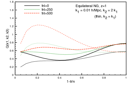
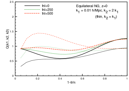
The equilateral model exhibits a different pattern compared to the local model. This behaviour can be seen more clearly in the upper panel of figure 10. There, we see that $Q$ is enhanced by non-Gaussianities in a way that it is highly dependent on $\theta$. The maximum of the effect occurs at $\theta\sim 2\pi/3$ which corresponds to equilateral configurations in this model and are responsible for the bump in this Figure near to $\theta\sim 0.8\pi$. Again, as in the local model, the effect of non-Gaussianities is greatly enhanced in the configuration $k_{2}/k_{1}=1$ while for higher $k_{1}$ the reduced bispectrum is much less sensitive to the effect of primordial NG regardless the value of the $f_{\rm NL}$ parameter.

Figure 10: The same as figure 8 for the equilateral model of primordial NG.

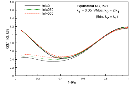
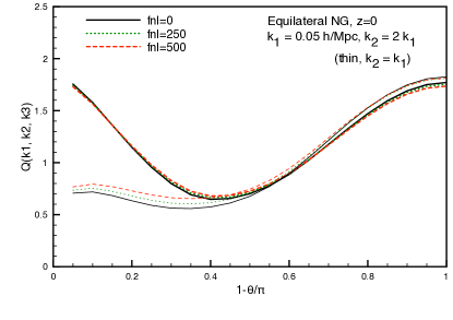
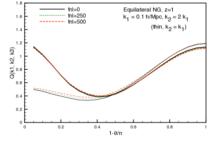
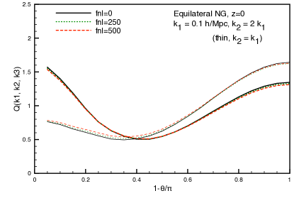
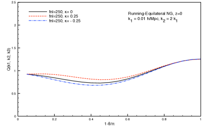
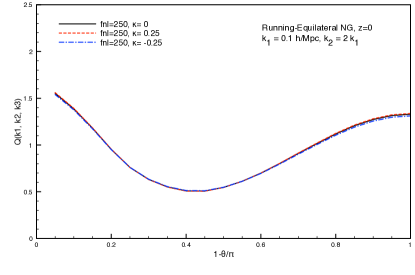
The result of the evaluation of the running $f_{\rm NL}$ equilateral case is shown in figure 11. In the configuration $k_{2}/k_{1}=2$, we evaluate for $\kappa=0,0.25,-0.25$. For $k_{1}=0.01\,h$/Mpc and $z=1$ we find a remarkable enhancement (suppression) for positive (negative) values of $\kappa$. For $k_{1}=0.1\,h$/Mpc and $z=0$ the effect is rather unnoticeable.

Figure 11: Reduced bispectrum for running $f_{\rm NL}$ with $f_{{\rm NL},P}=250$ and $\kappa=0$ (solid, black line), $\kappa=0.25$ (dashed, red line) and $\kappa=-0.25$ (dot-dashed, blue line).

5.3 Folded model

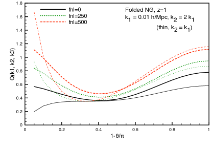
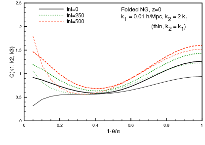
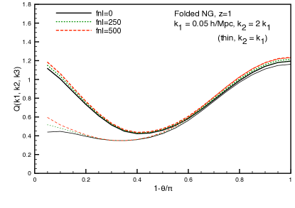
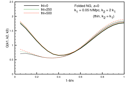
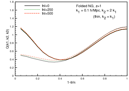
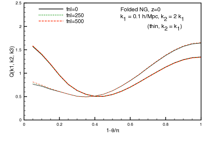
Contrary to the equilateral model, in the folded model, $Q$ is enhanced by the non-Gaussian contributions coming from the correlations among modes with almost collinear wave-vectors ($\theta=0,\,\pi$). This effect is maximized in the limit $\theta\rightarrow\pi$ (as in the local model) which corresponds to a folded configuration of the momentum-space triangle when $k_{2}\approx k_{3}\approx k_{1}/2$ (Figure 4). This effect can be seen in figure 12. As in the previus cases, the effect is maximized for small $k_{1}$ and for high redshift. For higher $k_{1}$ and lower redshift as in the bottom panel of figure 12 we see that the effect of this model of non-Gaussianities is tiny, regardless the value of $f_{\rm NL}$.

Figure 12: The same as figure 8 for the folded model of primordial NG.

6 Conclusions and Discussion

In this work we have studied several aspects related to the effects of primordial non-Gaussianities in gravitational clustering using the recently developed TRG method. We have discussed different shapes of primordial NG and evaluated their impact in the non-linear evolution of the power-spectrum and (reduced) bispectrum of matter density perturbations.

For the power-spectrum with some primordial NG present, we have compared our results to the ones of standard one-loop perturbation theory and N-body data. In the range $0.1\lesssim k\,{\rm Mpc}/h\lesssim 0.2$, the one-loop and the TRG method reproduce pretty well the data from the N-body simulations of Ref. [54] while, for $k\gtrsim 0.2\,h$/Mpc, the one-loop prediction begins to show some inaccuracies which are within the $\lesssim 2$ % level. The non-linear growth of the power-spectrum is more suppressed in the one-loop calculation than in the TRG calculation. The differences between the two approaches becomes more evident on smaller scales and lower redshifts, where the TRG offers a noticeable improvement with respect to the one-loop but still with a deviation from the N-body data. We expect that such deviations can be reduced if we take into account the “vertex corrections” including the trispectrum in the system of equations as we discussed in the Introduction. On general grounds, we expect that the effects arising from vertex corrections will become relevant for higher wavenumbers and that they will help to extend the range of validity of wavenumbers to larger values. We have also computed the reduced bispectrum for various shapes of NG. As stressed in Ref. [26], the reduced bispectrum is a powerful probe of NG. There the authors performed a Fisher matrix analysis to study the smallest value of the paramater $f_{\rm NL}$ measurable in high-redshift galaxy survays for local and equilateral shapes, after marginalizing over the bias parameters. At the tree-level the signal-to-noise ratio $(S/N)^{2}$ scales like (the sum over momenta forming a triangle of) $B^{2}(k_{1},k_{2},k_{3})/P(k_{1})P(k_{2})P(k_{3})$. For a local shape of NG, $k_{1}\ll k_{2}\sim k_{3}$, $B^{2}(k_{1},k_{2},k_{3})/P(k_{1})P(k_{2})P(k_{3})\sim P(k_{1})$. Non-linearities enter in the determination of the maximum wavenumber $k_{\rm max}$ at which one computes $(S/N)\sim f^{\rm loc}_{\rm NL}\,k_{\rm max}^{3/2}$. For the equilateral shape, $k_{1}\sim k_{2}\sim k_{3}$, and again at the tree level, the signal-to-noise ratio scales like $(S/N)\sim f^{\rm eq}_{\rm NL}\,k_{\rm max}^{5/2}\,P^{1/2}(k_{\rm max})\sim f^{\rm eq}_{\rm NL}\,k_{\rm max}$. Going beyond the linear order through the TRG method one should compute the full Fisher matrix and therefore $(\partial B(k_{1},k_{2},k_{3})/\partial f_{\rm NL})^{2}$. In this case the non-linear effects cannot be neglected. We leave this and other issues, such as the inclusion of the trispectrum, for future work.

References

- [1] M. Crocce and R. Scoccimarro, “Renormalized Cosmological Perturbation Theory,” Phys. Rev. D 73 (2006) 063519 [arXiv:astro-ph/0509418].
- [2] M. Crocce and R. Scoccimarro, “Memory of Initial Conditions in Gravitational Clustering,” Phys. Rev. D 73 (2006) 063520 [arXiv:astro-ph/0509419].
- [3] P. McDonald, “Dark matter clustering: a simple renormalization group approach,” Phys. Rev. D 75 (2007) 043514 [arXiv:astro-ph/0606028]; ibidem “Clustering of dark matter tracers: renormalizing the bias parameters,” Phys. Rev. D 74 (2006) 103512 [Erratum-ibid. D 74 (2006) 129901] [arXiv:astro-ph/0609413].
- [4] F. Bernardeau, S. Colombi, E. Gaztanaga and R. Scoccimarro, “Large-scale structure of the universe and cosmological perturbation theory,” Phys. Rept. 367 (2002) 1 [arXiv:astro-ph/0112551].
- [5] P. Valageas, “Dynamics of gravitational clustering I. Building perturbative expansions,” arXiv:astro-ph/0107015; “Dynamics of gravitational clustering II. Steepest-descent method for the quasi-linear regime,” arXiv:astro-ph/0107126.
- [6] T. Matsubara, “Resumming Cosmological Perturbations via the Lagrangian Picture: One-loop Results in Real Space and in Redshift Space,” Phys. Rev. D 77 (2008) 063530 [arXiv:0711.2521 [astro-ph]]; “Nonlinear perturbation theory with halo bias and redshift-space distortions via the Lagrangian picture,” Phys. Rev. D 78 (2008) 083519 [Erratum-ibid. D 78 (2008) 109901 ] [arXiv:0807.1733 [astro-ph]].
- [7] S. Matarrese and M. Pietroni, “Baryonic acoustic oscillations via the renormalization group,” Mod. Phys. Lett. A 23 (2008) 25 [arXiv:astro-ph/0702653].
- [8] S. Matarrese and M. Pietroni, “Resumming Cosmic Perturbations,” JCAP 06 (2007) 026 [arXiv:astro-ph/0703563].
- [9] K. Izumi and J. Soda, “Renormalized Newtonian Cosmic Evolution with Primordial Non-Gaussanity,” Phys. Rev. D 76 (2007) 083517 [arXiv:0706.1604 [astro-ph]].
- [10] M. Pietroni, “Flowing with Time: a New Approach to Nonlinear Cosmological Perturbations,” JCAP 10 (2008) 036 [arXiv:0806.0971 [astro-ph]].
- [11] J. Lesgourgues, S. Matarrese, M. Pietroni and A. Riotto, “Non-linear Power Spectrum including Massive Neutrinos: the Time-RG Flow Approach,” JCAP 06 (2009) 017 [arXiv:0901.4550 [astro-ph.CO]].
- [12] J. Carlson, M. White and N. Padmanabhan, “A critical look at cosmological perturbation theory techniques,” Phys. Rev. D 80 (2009) 043531 [arXiv:0905.0479 [astro-ph.CO]].
- [13] V. Acquaviva, N. Bartolo, S. Matarrese and A. Riotto, “Second-order cosmological perturbations from inflation,” Nucl. Phys. B 667 (2003) 119 [arXiv:astro-ph/0209156].
- [14] J. Maldacena, “Non-Gaussian features of primordial fluctuations in single field inflationary models,” JHEP 05 (2003) 013 [arXiv:astro-ph/0210603].
-
[15]
N. Bartolo, E. Komatsu, S. Matarrese and A. Riotto, Phys. Rept. 402 (2004)
103 [arXiv:astro-ph/0406398];
E. Komatsu et al., “NG as a Probe of the Physics of the Primordial Universe and the Astrophysics of the Low Redshift Universe,” arXiv:0902.4759 [astro-ph.CO]. - [16] S. Matarrese, F. Lucchin and S. A. Bonometto, “A Path Integral Approach To Large Scale Matter Distribution Originated By Nongaussian Fluctuations,” Astrophys. J. 310 (1986) L21.
- [17] B. Grinstein and M. Wise, “Nongaussian fluctuations and the correlations of galaxies or rich clusters of galaxies,” Astrophys. J. 310 (1986) 19.
- [18] F. Lucchin, S. Matarrese and N. Vittorio, “Scale invariant clustering and primordial biasing,” Astrophys. J. 330 (1988) L21.
- [19] L. Moscardini, S. Matarrese, F. Lucchin and A. Messina, “NonGaussian initial conditions in cosmological N body simulations: 2. Cold dark matter models,” Mon. Not. Roy. Astron. Soc. 248 (1991) 424.
- [20] K. Koyama, J. Soda and A. Taruya, “Constraints on a non-gaussian () CDM model,” Mon. Not. Roy. Astron. Soc. 310 (1999) 1111 [arXiv:astro-ph/9903027].
- [21] S. Matarrese, L. Verde, and R. Jimenez, “The abundance of high-redshift objects as a probe of non-Gaussian initial conditions,” Astrophys. J. 541 (2000) 10 [arXiv:astro-ph/0001366].
- [22] J. Robinson and J. Baker, “Evolution of the cluster abundance in non-Gaussian models,” Mon. Not. Roy. Astron. Soc. 311, 781 (1999).
- [23] J. Robinson, E. Gawiser and J. Silk, “Constraining Primordial Non-Gaussianity With the Abundance of High Redshift Clusters,” Astrophys. J. 532 (2000) 1 [arXiv:astro-ph/9906156].
- [24] M. Maggiore and A. Riotto, “The halo mass function from the excursion set method. III. First principle derivation for non-Gaussian theories,” arXiv:0903.1251 [astro-ph.CO].
- [25] M. Maggiore and A. Riotto, “The Halo Mass Function from Excursion Set Theory with a Non-Gaussian Trispectrum,” arXiv:0910.5125 [astro-ph.CO].
- [26] E. Sefusatti and E. Komatsu, “The bispectrum of galaxies from high-redshift galaxy surveys: Primordial non-Gaussianity and non-linear galaxy bias,” Phys. Rev. D 76 (2007) 083004 [arXiv:0705.0343 [astro-ph]].
- [27] C. Carbone, L. Verde and S. Matarrese, “Non-Gaussian halo bias and future galaxy surveys,” Astrophys. J. 684 (2008) 1 [arXiv:0806.1950 [astro-ph]].
- [28] L. Verde and S. Matarrese, “Detectability of the effect of Inflationary non-Gaussianity on halo bias,” Astrophys. J. 706 (2009) L91 [arXiv:0909.3224 [astro-ph.CO]].
- [29] N. Dalal, O. Dore, D. Huterer and A. Shirokov, “The imprints of primordial non-gaussianities on large-scale structure: scale dependent bias and abundance of virialized objects,” Phys. Rev. D 77 (2008) 123514 [arXiv:0710.4560 [astro-ph]].
- [30] S. Matarrese and L. Verde, “The effect of primordial non-Gaussianity on halo bias,” Astrophys. J. 677(2008) L77 [arXiv:0801.4826 [astro-ph]].
- [31] A. Slosar, C. Hirata, U. Seljak, S. Ho and N. Padmanabhan, “Constraints on local primordial non-Gaussianity from large scale structure,” JCAP 0808 (2008) 031 [arXiv:0805.3580 [astro-ph]].
- [32] N. Afshordi and A. J. Tolley, “Primordial non-gaussianity, statistics of collapsed objects, and the Integrated Sachs-Wolfe effect,” Phys. Rev. D 78 (2008) 123507 [arXiv:0806.1046 [astro-ph]].
- [33] N. Bartolo, S. Matarrese and A. Riotto, “Signatures of Primordial Non-Gaussianity in the Large-Scale Structure of the Universe,” JCAP 10 (2005) 010 [arXiv:astro-ph/0501614].
- [34] L. Senatore, K. M. Smith and M. Zaldarriaga, “Non-Gaussianities in Single Field Inflation and their Optimal Limits from the WMAP 5-year Data,” arXiv:0905.3746 [astro-ph.CO].
- [35] A. Taruya, K. Koyama and T. Matsubara, “Signature of Primordial Non-Gaussianity on Matter Power Spectrum,” Phys. Rev. D 78 (2008) 123534 [arXiv:0808.4085 [astro-ph]].
- [36] E. Sefusatti, “1-loop Perturbative Corrections to the Matter and Galaxy Bispectrum with non-Gaussian Initial Conditions,” Phys. Rev. D 80 (2009) 123002 [arXiv:0905.0717 [astro-ph.CO]].
- [37] R. Scoccimarro, S. Colombi, J. N. Fry, J. A. Frieman, E. Hivon and A. Melott, “Nonlinear evolution of the bispectrum of cosmological perturbations,” Astrophys. J. 496 (1998) 586 [arXiv:astro-ph/9704075].
- [38] P. Catelan and L. Moscardini, “Kurtosis as a Non–Gaussian Signature of the Large–Scale Velocity Field,” Astrophys. J. 436 (1994) 5 [arXiv:astro-ph/9403035].
- [39] N. Bartolo, S. Matarrese and A. Riotto, “CMB Anisotropies at Second-Order II: Analytical Approach,” JCAP 01 (2007) 019 [arXiv:astro-ph/0610110].
- [40] A. L. Fitzpatrick, L. Senatore and M. Zaldarriaga, “Contributions to the Dark Matter 3-Pt Function from the Radiation Era,” arXiv:0902.2814 [astro-ph.CO].
- [41] J. R. Fergusson and E. P. S. Shellard, “The shape of primordial non-Gaussianity and the CMB bispectrum,” Phys. Rev. D 80 (2009) 043510 [arXiv:0812.3413 [astro-ph]].
- [42] E. Komatsu et al. [WMAP Collaboration], “Five-Year Wilkinson Microwave Anisotropy Probe (WMAP) Observations:Cosmological Interpretation,” Astrophys. J. Suppl. 180 (2009) 330 [arXiv:0803.0547 [astro-ph]].
- [43] A. Lewis, A. Challinor and A. Lasenby, “Efficient Computation of CMB anisotropies in closed FRW models,” Astrophys. J. 538 (2000) 473 [arXiv:astro-ph/9911177].
- [44] M. Alishahiha, E. Silverstein and D. Tong, “DBI in the sky,” Phys. Rev. D 70 (2004) 123505 [arXiv:hep-th/0404084].
- [45] D. Babich, P. Creminelli and M. Zaldarriaga, “The shape of non-Gaussianities,” JCAP 08 (2004) 009 [arXiv:astro-ph/0405356].
- [46] X. Chen, M. x. Huang, S. Kachru and G. Shiu, “Observational signatures and non-Gaussianities of general single field inflation,” JCAP 01 (2007) 002 [arXiv:hep-th/0605045].
- [47] R. Holman and A. J. Tolley, “Enhanced NG from Excited Initial States,” JCAP 05 (2008) 001 [arXiv:0710.1302 [hep-th]].
- [48] P. D. Meerburg, J. P. van der Schaar and P. S. Corasaniti, “Signatures of Initial State Modifications on Bispectrum Statistics,” JCAP 05 (2009) 018 [arXiv:0901.4044 [hep-th]].
- [49] X. Chen, “Running non-Gaussianities in DBI Inflation,” Phys. Rev. D 72 (2005) 123518 [arXiv:astro-ph/0507053].
- [50] M. LoVerde, A. Miller, S. Shandera and L. Verde, “Effects of Scale-Dependent NG on Cosmological Structures,” JCAP 04 (2008) 014 [arXiv:0711.4126 [astro-ph]].
- [51] E. Sefusatti, M. Liguori, A. P. S. Yadav, M. G. Jackson and E. Pajer, “Constraining Running NG,” arXiv:0906.0232 [astro-ph.CO].
- [52] C. T. Byrnes, K. Y. Choi and L. M. H. Hall, “Large non-Gaussianity from two-component hybrid inflation,” JCAP 02 (2009) 017 [arXiv:0812.0807 [astro-ph]].
- [53] C. T. Byrnes, S. Nurmi, G. Tasinato and D. Wands, “Scale dependence of local ,” arXiv:0911.2780 [astro-ph.CO].
- [54] A. Pillepich, C. Porciani and O. Hahn, “Universal halo mass function and scale-dependent bias from N-body simulations with non-Gaussian initial conditions,” arXiv:0811.4176 [astro-ph].
- [55] T. Giannantonio and C. Porciani, “Structure formation from non-Gaussian initial conditions: multivariate biasing, statistics, and comparison with N-body simulations,” arXiv:0911.0017 [astro-ph.CO].
- [56] M. Grossi, K. Dolag, E. Branchini, S. Matarrese and L. Moscardini, “Evolution of Massive Haloes in non-Gaussian Scenarios,” Mon. Not. Roy. Astron. Soc. 382 (2007) 1261 [arXiv:0707.2516 [astro-ph]]; “The mass density field in simulated non-Gaussian scenarios,” Mon. Not. Roy. Astron. Soc. 390 (2008) 438 [arXiv:0805.0276 [astro-ph]]; “Large-scale non-Gaussian mass function and halo bias: tests on N-body simulations,” Mon. Not. Roy. Astron. Soc. 398 (2009) 321 [arXiv:0902.2013 [astro-ph.CO]].
- [57] V. Desjacques, U. Seljak and I. Iliev, “Scale-dependent bias induced by local non-Gaussianity: A comparison to N-body simulations,” arXiv:0811.2748 [astro-ph]; V. Desjacques and U. Seljak, “Signature of primordial non-Gaussianity of -type in the mass function and bias of dark matter haloes,” arXiv:0907.2257 [astro-ph.CO].
- [58] T. Nishimichi, A. Taruya, K. Koyama and C. Sabiu, “Scale Dependence of Halo Bispectrum from Non-Gaussian Initial Conditions in Cosmological N-body Simulations,” arXiv:0911.4768 [astro-ph.CO].