What limits supercurrents in high temperature superconductors? A microscopic model of cuprate grain boundaries

The interface properties of high-temperature cuprate superconductors have been of interest for many years, and play an essential role in Josephson junctions, superconducting cables, and microwave electronics. In particular, the maximum critical current achievable in high-$T_{c}$ wires and tapes is well known to be limited by the presence of grain boundaries Mannhart , regions of mismatch between crystallites with misoriented crystalline axes. In studies of single, artificially fabricated grain boundaries the striking observation has been made that the critical current $J_{c}$ of a grain boundary junction depends exponentially on the misorientation angle Dimosetal88 . Until now microscopic understanding of this apparently universal behavior has been lacking. We present here the results of a microscopic evaluation based on a construction of fully 3D YBa₂Cu₃O_7-δ  grain boundaries by molecular dynamics. With these structures, we calculate an effective tight-binding Hamiltonian for the $d$-wave superconductor with a grain boundary. The critical current is then shown to follow an exponential suppression with grain boundary angle. We identify the buildup of charge inhomogeneities as the dominant mechanism for the suppression of the supercurrent.

To explain the exponential dependence of the critical current $J_{c}$ on the misorientation angle $\alpha$ Chaudhari and collaborators Chaudhari introduced several effects which can influence the critical current that are particular to high-temperature superconductor (HTS) grain boundaries (GB). First, a variation with angle can arise from the relative orientation of the $d$-wave order parameters pinned to the crystal lattices on either side of the boundary. This scenario was investigated in detail by Sigrist and Rice SigristRice . However, such a modelling cannot explain the exponential suppression of the critical current over the full range of misorientation angles. Secondly, dislocation cores, whose density grows with increasing angle, can suppress the total current. A model assuming insulating dislocation cores which nucleate antiferromagnetic regions and destroy superconducting order was studied by Gurevich and Pashitskii Gurevich . However, for grain boundary angles beyond approximately 10^∘ when the cores start to overlap this model fails. Finally, variations of the stoichiometry in the grain boundary region, such as in the oxygen concentration, may affect the scattering of carriers and consequently the critical current. Stolbov and collaborators Stolbov as well as Pennycook and collaborators Pennycook have examined the bond length distribution near the grain boundary and calculated the change in the density of states at the Fermi level, or the change in the Cu valence, respectively. In the latter work the authors used the reduced valences to define an effective barrier near the boundary whose width grows linearly with misorientation angle.

A critical examination of the existing models shows that the difficulty of the longstanding HTS “grain boundary problem” arises from the multiple length scales involved: atomic scale reconstruction of the interface, the electrostatic screening length, the antiferromagnetic correlation length, and the coherence length of the superconductor. Thus it seems likely that only a multiscale approach to the problem can succeed.

Our goal in this paper is to simulate, in the most realistic way possible, the nature of the actual grain boundary in a cuprate HTS system, in order to characterize the multiple scales which cause the exponential suppression of the angle dependent critical current. To achieve this goal we proceed in a stepwise fashion, first simulating the atomic structure of realistic YBCO grain boundaries and assuring ourselves that our simulations are robust and duplicate the systematics of actual grain boundaries. Subsequently we construct an effective disordered tight-binding model, including $d$-wave pairing, whose parameters depend on the structures of the simulated grain boundaries in a well-defined way. Thus for any angle it will be possible to calculate the critical current; then, for a given pairing amplitude (reasonably well known from experiments on bulk systems) the form of $J_{c}(\alpha)$ and its absolute magnitude is calculated.

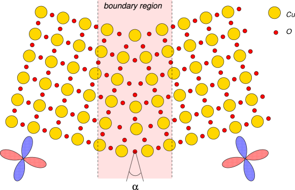
Figure 1: Schematic of an HTS symmetric grain boundary. The misorientation angle $\alpha$ and the orientation of the $d$-wave order parameters are indicated.

We simulate YBCO grain boundaries by a molecular dynamics (MD) procedure which has been shown to reproduce the correct structure and lattice parameters of the bulk YBa₂Cu₃O_7-δ  crystal Zhang , and adapt techniques which were successfully applied to twist grain boundaries in monocomponent solids Phillpot . We only sketch the procedure here, and postpone its details to the supplementary information and a longer publication. The method uses an energy functional within the canonical ensemble

$$H=\frac{1}{2}\sum_{i=1}^{N}\sum_{\alpha=1}^{3}m_{i}\dot{r}_{i,\alpha}^{2}+\frac{1}{2}\sum_{i=1}^{N}\sum_{j=1,j\neq i}^{N}U(r_{ij}),$$ (1)

where $m_{i}$ is the mass of the ion and $U(r_{ij})$ is the effective potential between ions, taken to be of the form $U(r_{ij})=\Phi(r_{ij})+V(r_{ij})$. Here $V(r)$ is the screened Coulomb interaction $V(r)=\pm e^{-\kappa r}{Z^{2}e^{2}}/({4\pi\epsilon_{0}}{r})$ with screening length $\kappa^{-1}$, and $\Phi(r)$ is a short range Buckingham potential $\Phi(r)=A\exp(-r/\rho)-C/r^{6}$. We take the parameters $A$, $\rho$ and $C$ from Ref. Zhang, , and the initial lattice constants are $a=3.82$ Å, $b=3.89$ Å and $c=11.68$ Å. To construct a grain boundary with well defined misorientation angle, we must fix the ion positions on both sides far from the boundary, and ensure that we have a periodic lattice structure along the grain boundary and also along the $c$-axis direction. Therefore we apply periodic boundary conditions in the molecular dynamics procedure in the direction parallel to the GB and also in the $c$-axis direction. In the direction perpendicular to the GB only atomic positions with a distance smaller than six lattice constants from the GB are reconstructed. This method restricts our consideration to grain boundary angles that allow a commensurate structure parallel to the GB, e.g. angles $\alpha=2\cdot\arctan[{N_{1}a}/({N_{2}b})],\leavevmode\nobreak\ N_{1},N_{2}\in\mathbf{N}$ gbangles .

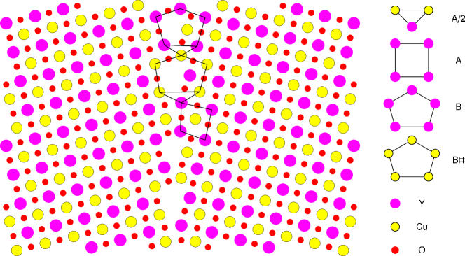
Figure 2: Top view of a calculated (410) grain boundary. Here only the Y and the CuO₂ layers are shown. The dots show the position of Y ions (magenta), Cu ions (yellow), and O ions (red). Structural units are indicated by solid black lines. For this particular angle we find a sequence of the form A(A/2)B#(A/2)B, in agreement with the experimental results given in Table 1 of Ref. Pennycook, (for notation see this reference).

An important step to be taken before starting the reconstruction of the GB is the initial preparation of the GB. Since we use a fixed number of ions at the GB within the molecular dynamics algorithm we have to initialize it with the correct number of ions. If we start with two perfect but rotated crystals on both sides of the interface, in which all ions in the half space behind the imaginary boundary line are cut away, we find that several ions are unfavorably close to each other. Here we have to use a set of selection rules to replace two ions by a single one at the grain boundary. These selection rules have to be carefully chosen for each type of ion since they determine how many ions of each type are present in the grain boundary region; the rules are detailed in the supplementary information. Ultimately they should be confirmed by a grand canonical MD procedure. However, such a procedure for a complex multicomponent system as the YBCO GB is technically still not feasible. While the selection rules are ad hoc in nature, we emphasize that they are independent of misorientation angle, and reproduce very well the experimental TEM structures Pennycook .

With the initial conditions established, the MD equations of motion associated with Eq. 1 are iterated until all atoms are in equilibrium. As an example, we show in Fig. 2 the reconstructed positions of Y, Cu, and O ions for a (410) boundary. We emphasize that the MD simulation is performed for all the ions in the YBCO full 3D unit cells of two misoriented crystals except for a narrow “frame” consisting of ions that are fixed to preserve the crystalline order far from the grain boundary. The sequence of typical structural units identified in the experiments Pennycook is also indicated and we find excellent agreement.

We next proceed to construct an effective tight-binding model which is restricted to the Cu sites, the positions of which were determined through the algorithm described. We calculate hopping matrix elements $t_{ij}$ of charge carriers (holes) up to next nearest neighbor positions of Cu ions. The Slater-Koster method is used to calculate the directional dependent orbital overlaps of Cu-$3d$ and O-$2p$ orbitals SlaterKoster ; Harrison . The effective hopping between Cu positions is a sum of direct orbital overlaps and hopping via intermediate O sites, where the latter is calculated in 2nd order perturbation theory. For the homogeneous lattice, these parameters agree reasonably well with the numbers typically used in the literature for YBCO. Exact values and details of the procedure are given in the supplementary information. Results for a (410) grain boundary are shown in Fig. 3. Note the largest hopping probabilities across the grain boundary are associated with the 3fold coordinated Cu ions which are close to dislocation cores. The inhomogeneities introduced through the distribution of hopping probabilities along the boundary induce scattering processes of the charge carriers and consequently contribute to an “effective barrier” at the grain boundary. We note that the angular dependence of the critical current $J_{c}(\alpha)$ is not directly related to the changes in averaged hopping parameters observed for different misalignment angles. In fact we found that the variation of the hopping probabilities with boundary angle cannot account by itself for the exponential dependence of $J_{c}(\alpha)$ over the whole range of misalignment angles.

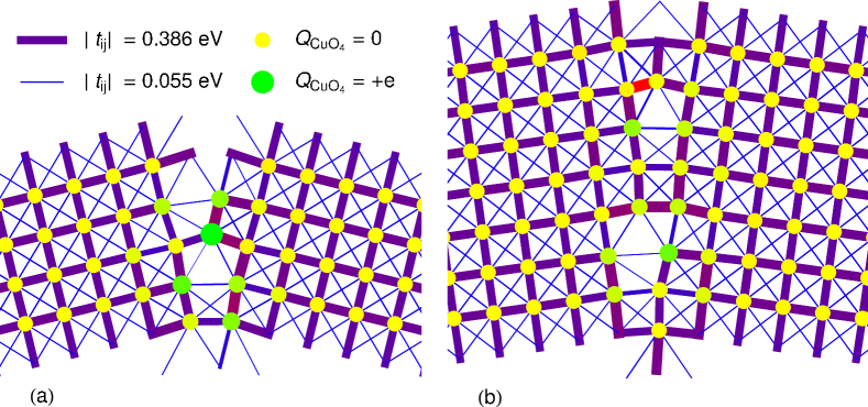
Figure 3: Tight-binding model for the CuO₂ plane. Hopping values between the Cu ions calculated from the interatomic matrix elements for a (410) grain boundary (a) and for a (710) grain boundary (b). The line thickness shows the hopping amplitudes and the color and size of the copper sites illustrate the on-site potential.

The structural imperfection at the grain boundary will necessarily lead to charge inhomogeneities that will contribute—in a similar way as the reduced hopping probabilities—to the effective barrier that blocks the superconducting current over the grain boundary. We include these charge inhomogeneities into the calculations by considering them in the effective Hamiltonian as on-site potentials on the Cu sites. To accomplish this we utilize the method of valence bond sums. The basic idea is to calculate the bond valence of a cation by

$$V_{i}=\sum_{j}\exp\left(\frac{r_{0}-r_{ij}}{B}\right)$$ (2)

where $j$ runs over all neighboring anions, in our case the neighboring negatively charged oxygen ions. The parameter $B=0.37$ Å is a universal constant in the bond valence theory, while $r_{0}$ is different for all cation-anion pairs and also depends on the formal integer oxidation state of the cation (the values are listed in Ref. Chmaissem, ). Strong deviations from the formal valence reveal strain or even an incorrect structure. This procedure is straightforward in the case of the Y³⁺ and Ba²⁺ ions, while it is slightly more complicated for the Cu ions, because they have more than one formal integer oxidation state Brown ; Chmaissem . We show in Fig. 4 the distribution of charges at the (410) grain boundary obtained. We also calculate by similar methods the oxidation state of the oxygen ions. Here, charge neutrality is ensured because the already determined cation valences are used.

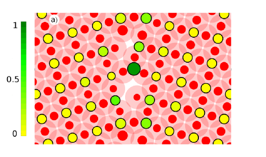
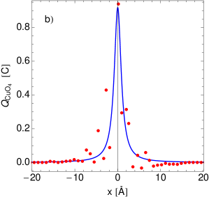
Figure 4: Charging of the CuO₄ squares. a) Charge distribution on copper (yellow/green) and oxygen (red) sites at a 410 boundary. The diameter of the circles is a measure for positive (copper) or negative (oxygen) charge, as determined by the bond valence analysis. The color of the copper sites represents the charging of the corresponding CuO₄ squares as described by Eq. 3, with green circles referring to a positive charge compared to the bulk charge (see color scale). The transparent red circles represent the oxygen contributions to the CuO₄ charge. b) Plot of average charge on squares vs. distance from grain boundary (red points), and fit by a Lorentzian (blue line).

In the next step we account for the effect of broken Cu-O bonds at the grain boundary that give rise to strong changes of the electronic configuration of the Cu atoms as well as of the electronic screening of charges, as shown in first principle calculations Stolbov . Unfortunately there is no straightforward way to include these changes in the electronic configuration into a purely Cu-based tight-binding Hamiltonian. On the other hand we know that the additional holes doped into the CuO₂ planes form Zhang-Rice singlets residing on a CuO₄ square rather than on a single Cu site ZhangRice , and are therefore affected not only by the charge of the Cu ion but also by the charge of the surrounding oxygens. Modelling this situation, we use a phenomenological potential to sum the Cu and the O charges to obtain an effective charge of the CuO₄ square. This effective charge is taken as

$$Q_{\textrm{CuO}_{4}}(i)=Q_{\textrm{Cu}}(i)+A\sum_{j}Q_{0}(j)e^{-r_{ij}^{2}/\lambda^{2}},$$ (3)

where $A$ and $\lambda$ are two constants chosen to yield a neutral Cu site if 4 oxygen atoms are close to the average Cu-O distance. Correspondingly, the energy cost of a Cu site that has only 3 close oxygen neighbors instead of all 4 neighbors, is strongly enhanced. Thus, the broken Cu-O bonds induce strong charge inhomogeneities in the “void” regions of the grain boundary, mainly described by pentagonal structural units, while Cu sites belonging to “bridge” regions with mostly quadrangular structural units have charge values close to their bulk values.

Finally we have to translate the charge on the Cu sites (or better CuO₄ squares) into effective on-site lattice potentials. The values of screening lengths in the cuprates, and particularly near grain boundaries, are not precisely known, but near optimal doping they are of order of a lattice spacing or less. We adopt the simplest approach and assume a 3D Yukawa-type screening with phenomenological length parameter $\ell$ of this order, and find a potential integrated over a unit cell $V_{0}$ of

$$\frac{V_{0}}{a^{2}\bar{q}}\approx 4\pi\leavevmode\nobreak\ (a_{0}\ell)\leavevmode\nobreak\ \mathrm{Ryd}\approx 10\leavevmode\nobreak\ \mathrm{eV},$$ (4)

where $\bar{q}$ is the charge in units of the elementary charge, $a_{0}$ is the Bohr radius, and $\ell$ is taken to be $2$ Å while $a=4$ Å. Thus we find a surplus charge of a single elementary charge integrated over a unit cell to produce an effective potential of around $10$ eV. In the following we will use an effective potential of either 6 or 10 eV, reflecting the uncertainty in this parameter. The value of the effective potential will affect the scale of the final critical current.

To calculate the order parameter profile and the current across the grain boundary we solve the Bogoliubov-de Gennes mean field equations of inhomogeneous superconductivity self-consistently. The Hamiltonian is

$$\hat{H}=\sum_{i}\epsilon_{i}\hat{n}_{i\sigma}-\sum_{ij\sigma}t_{ij}\hat{c}_{i\sigma}^{\dagger}\hat{c}_{j\sigma}+\sum_{ij}\left(\Delta_{ij}\hat{c}_{i\uparrow}^{\dagger}\hat{c}_{j\downarrow}^{\dagger}+\mathrm{h.c.}\right),$$ (5)

where the effective hopping parameters $t_{ij}$ are determined for a given grain boundary by the procedure described above and the onsite energies $\epsilon_{i}=u_{i}-\mu$ are a sum of the effective charge potentials $u_{i}$ and the chemical potential $\mu$. Performing a Bogoliubov transformation, we find equations for the particle and hole amplitudes $u_{n}$ and $v_{n}$

$$\sum_{j}\left(\begin{array}[]{cc}H_{ij}&\Delta_{ij}\\ {\Delta}_{ij}^{*}&-H_{ij}\end{array}\right)\left(\begin{array}[]{c}u_{n}(j)\\ v_{n}(j)\end{array}\right)=E_{n}\left(\begin{array}[]{c}u_{n}(i)\\ v_{n}(i)\end{array}\right)$$ (6)

with

$$H_{ij}=\epsilon_{i}\delta_{ij}-t_{ij}$$ (7)

The self-consistency equation for the $d$-wave order parameter is then

$$\Delta_{ij}=\frac{V_{ij}}{2N_{\textrm{sc}}}\sum_{k_{y}}\sum_{n}\left[u_{n}(r_{i})v_{n}^{*}(r_{j})f(-E_{n})-v_{n}^{*}(r_{i})u_{n}(r_{j})f(E_{n})\right],$$ (8)

where we use $N_{\textrm{sc}}$ supercells in the direction parallel to the GB and $k_{y}$ is the corresponding Bloch wave vector. We adjust the chemical potential $\mu$ to ensure a fixed carrier density in the superconducting leads corresponding to 15$\%$ hole doping. The definition of the $d$-wave pair potential $V_{ij}$ in the vicinity of the grain boundary is not straightforward since the bonds connecting a Cu to its neighbors are not exactly oriented perpendicular to each other. We use a model that ties the strength of the pairing on a given bond to the size of the hopping on the bond, as well as to the charge difference across it, as detailed in the supplementary information. The final results for the critical current are not sensitive to the exact model employed.

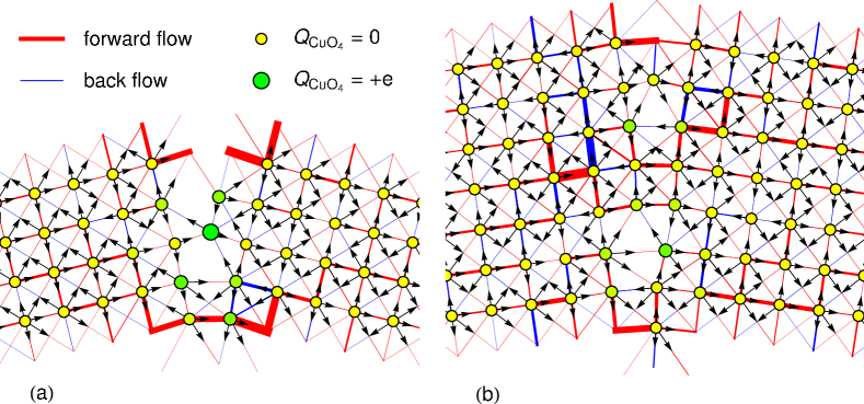
Figure 5: Supercurrent distribution. The current pattern in the vicinity of a (410) (a) and a (710) GB (b). The arrows only display the direction of the current, the red lines denote current flowing from left to right, blue lines denote current from right to left. The line thickness shows the current strength, while the point size and color of the Cu sites correspond to the on-site potential.

With these preliminaries, the current itself can finally be calculated by imposing a phase gradient across the sample (see, e.g. Ref. AndersenJc, for details) from the eigenfunctions $u_{n},v_{n}$ and eigenvalues $E_{n}$ of the BdG equations for the grain boundary,

$$\frac{j(r_{i},r_{j})}{e/\hbar}=-\frac{2it_{ij}}{N_{\textrm{sc}}}\sum_{k_{y}}\sum_{n}\left[u_{n}^{*}(r_{i})u_{n}(r_{j})f(E_{n})+v_{n}(r_{i})v_{n}^{*}(r_{j})f(-E_{n})-\mathrm{h.c.}\right]$$ (9)

The critical current $J_{c}$ is defined as the maximum value of the current as a function of the phase. In the tunnelling limit, when the barrier is large, this relationship is sinusoidal so the maximum current occurs at phase $\pi/2$. However, for very low angle grain boundaries we observe deviations from the tunnelling limit, i.e. higher transparency grain boundaries with non sinusoidal current-phase characteristics, although for the parameters studied here these deviations are rather small.

It is instructive to examine the spatial pattern of supercurrent flow across a grain boundary, which is far from simple, as illustrated in Fig. 5. Along many bonds even away from the boundary, the current flows backwards or runs in closed loops around the squares. The flow appears to be dominated by large contributions between the regions which resemble classical dislocation cores. In most of our simulated grain boundaries we do not observe true $\pi$ junction behavior, characterized by an overall negative critical current. To derive the total current density across a 2D cross section parallel to the grain boundary at $x=0$ we sum up all contributions of $j(r_{i},r_{j})$ for which $x_{i}>0$ and $x_{j}<0$, with $x=0$ the $x$ coordinate (perpendicular to the interface) of the boundary, and normalize by the period length of the grain boundary structure $p=a/\sin\alpha$.

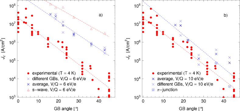
Figure 6: Angle dependence of the critical current. The critical current $J_{c}$ as a function of the grain boundary angle $\alpha$ for screening lengths $\ell=1.2$ Å (a) and 2 Å (b). Here the red points denote experimental results for YBCO junctions taken from Ref. Mannhart, , the light blue crosses show theoretical results for differently reconstructed GBs, the dark blue crosses show averaged theoretical values, and the light red triangles show “hypothetical” $s$-wave results. The dashed red and blue lines are exponential fits to the experimental and theoretical data, respectively.

This calculation is in principle capable of providing the absolute value of the critical current. To accomplish this, we have to normalize the current per grain boundary length by the height of the crystal unit cell $c$ and multiply it by the number of CuO planes per unit cell $N_{\textrm{UC}}$, e.g. for the YBCO compound under consideration $c=11.7$ Å, $N_{\textrm{UC}}=2$,

$$j_{c}(x_{0})=\frac{N_{\textrm{UC}}}{pc}\sum_{i<j,x_{i}<0<x_{j}}j(r_{i},r_{j})$$ (10)

To account for the difference of the calculated gap magnitude from its experimental value we multiply the current by a factor of $\Delta_{\textrm{exp}}/\Delta_{0}$, where $\Delta_{\textrm{exp}}$ is the experimentally measured order parameter and $\Delta_{0}$ is its self-consistently determined bulk value. We have checked that at low temperatures $T\ll T_{c}$ an approximately linear scaling of the critical current as a function of the order parameter holds true for all grain boundary angles.

In Fig. 6, the critical current is plotted as a function of misorientation angle for a set of grain boundary junctions from (710) to (520) which we have simulated. All model parameters are fixed for the different junctions, except for a range of values affecting the initial conditions of the grain boundary reconstruction, which resulted in slightly different structures with the same misorientation angle $\alpha$. Intriguingly, the variability of our simulated junctions is quite similar to the variability of actual physical samples as plotted in Fig. 6. For two different choices of the screening length $\ell$, we see that the dependence on misorientation angle is exponential. Since in our picture this parameter directly affects the strength of the barrier, it is also natural that it should affect the exponential decay constant, as also shown by the Figure. The value of $\ell$ which gives the correct slope of the log plot yields a critical current which exceeds the experimental value by an order of magnitude. We speculate that the effect of strong correlations (see Ref. Freericks, and references therein), not yet included in this theory, may account for this discrepancy, given that a suppression by an order of magnitude was already shown for (110) junctionsAndersen_AF_SC . We show in addition results for “hypothetical” $s$-wave junctions using the same model parameters as for the $d$-wave junctions. We simply replaced the bond-centered pair potential by an on-site pair potential resulting in an isotropic $s$-wave state. Although it is one order of magnitude larger, the critical current for the $s$-wave junction still shows a similar exponential dependence on the grain boundary angle. We emphasize that this model does not reflect the situation in a “real” $s$-wave superconductor like niobium or lead, that do not show an exponential angle dependence of the grain boundary current, since it is based on the microscopic structures of a CuO₂ plane.

Our multiscale analysis of the grain boundary problem of HTS suggests that the primary cause of the exponential dependence on misorientation angle is the charging of the interface near defects which resemble classical dislocation coresGurevich , leading to a porous barrier where weak links are distributed in a characteristic way which depends on the global characteristics of the interface at a given angle (structure of defects, density of dislocations, etc.). The $d$-wave order parameter symmetry and the nature of the atomic wave functions at the boundary which modulate the hopping amplitudes do not appear to be essential for the functional form of the angle dependence although they cannot be neglected in a quantitative analysis. As such, we predict that this type of behavior may be observed in other classes of complex superconducting materials. Very recently, a report of similar tendencies in ferropnictide grain boundary junctions appeared to confirm thisLarbalestier . It will be interesting to use the new perspective on the longstanding problem to try to understand how Ca doping of the grain boundaries is able to increase the critical current by large amountsHammerl , and to explore other chemical and structural methods of accomplishing the same goal.

Appendix A Grain boundary reconstruction using molecular dynamics techniques

The first step in our multiscale approach to determine the critical current over a realistic tilt grain boundary (GB) is the modelling of the microscopically disordered region in the vicinity of the seam of the two rotated half crystals. Since the disorder introduced by the mismatch of the two rotated lattices extends far into the leads on both sides of the GB plane, simulations have to include a large number of atoms and it is very difficult to perform them with high precision ab initio methods as for example density function theory (DFT) Schuster . Here we have employed a molecular dynamics technique to simulate the reconstruction of the ionic positions in the vicinity of the GB starting from an initial setup containing a realistic stoichiometry of each of the different ions. In the following we will present the details of the calculational scheme.

A.1 The initial setup of the grain boundary

The simplest way of modelling a tilt grain boundary is to stitch two perfect crystals together that are rotated into one another around an axis in the plane of the GB perpendicular to a lattice plane; atoms which cross into the region of space initially occupied by the other crystal are then eliminated (see Fig. 7 a). If we examine the structures constructed in this way we find on the one hand that some ions are left unphysically close to each other, while on the other hand large “void” regions may also remain. Since a molecular dynamics scheme employing an energy functional in the canonical ensemble does not allow for the creation and annihilation of ions in the GB region these faults in the setup will persist during the reconstruction process. To improve the initial structures we develop a set of “selection rules”: (i) We introduce an overlap of the two crystals, extending them into a region behind the virtual GB plane to prevent the creation of “void” regions. (ii) We replace two ions that are too close to each other by a single one at the GB. Due to the different ionic radii, the different multiplicities and the different internal positions these “selection rules” have to be adjusted for every ion in the unit cell in order to reproduce the correct stoichiometry found in TEM experiments Pennycook . In Table 1 we show the maximum overlap of ionic positions behind the GB plane as well as the minimum distance between two ions allowed before replacing them by a single ion at the GB. These values have proven to reproduce the experimentally observed GB structures for all misorientation angles examined within this work. An example of such a constructed GB is shown in Fig. 7 b).

	Y3+	Ba2+	Cu2+ (CuO2)	Cu2+ (CuO)
ov [$a$]	0.15	0.2	0.15	0.15
$d_{\mathrm{min}}$ [$a$]	0.4	0.4	0.42	0.4
	O2- (BaO)	O2- (CuO2: $a$)	O2- (CuO2: $b$)	O- (CuO)
ov [$a$]	0.08	0.08	0.09	0.08
$d_{\mathrm{min}}$ [$a$]	0.3	0.35	0.3	0.3

Table 1: The maximum overlap behind the GB plane and the minimum distance allowed between two ionic positions itemised by the different ion types. The distances are given in units of the lattice constant $a=3.82$ Å.

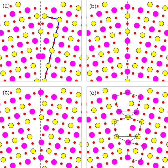
Figure 7: The different steps in the reconstruction of a symmetric (410) GB: (a) Two half crystals rotated and cut behind the virtual GB plane (dashed line), (b) Initial setup of the GB using the “selection rules” outlined in the text, (c) Reconstructed GB using molecular dynamics, (d) Identification of basic structural unitsPennycook . The blue line in (a) visualizes the classification of the ($mn0$) GB with $m=4$ and $n=1$.

A.2 The molecular dynamics procedure

The GB structures determined by applying the “selection rules” described in detail in the previous section are now used to initialize the molecular dynamics process. For monocomponent solids a method of zero temperature quenching has been successfully applied for the reconstruction of high-angle twist GBs Phillpot . Since this method uses an energy functional within the grand-canonical ensemble it allows besides the movement of the atomic position also the creation and annihilation of atoms. For multicomponent systems like the complicated perovskite-type structures of the high-$T_{c}$ superconductors this method is not readily applicable. Therefore we choose a different approach using an energy functional in the canonical ensemble with a fixed number of ions. Here we can write the Lagrangian as

$$\mathcal{L}=\frac{1}{2}\sum_{i=1}^{M}\sum_{\alpha=1}^{3}m_{i}\dot{r}_{i\alpha}^{2}-\frac{1}{2}\sum_{i=1}^{M}\sum_{j=1,j\neq i}^{M}U(r_{ij}),$$ (11)

and the Euler-Lagrange equations follow as the equations of motion for the ions

$$m_{i}\ddot{r}_{i,\alpha}=-\frac{1}{2}\sum_{j=1,j\neq i}^{M}\frac{\partial U(r_{ij})}{\partial r_{i,\alpha}}.$$ (12)

One of the main tasks is now the correct choice of model potentials to ensure that the crystal structure of YBa₂Cu₃O₇ (YBCO) is correctly reproduced for a homogeneous sample. Here we use Born model potentials with long range Coulomb interactions and short range terms of the Buckingham form

$$U(r_{ij})=\Phi(r_{ij})+V(r_{ij}).$$ (13)

For the Coulomb interaction we can write the potential as

$$V(r)=\pm e^{-\kappa r}\frac{1}{4\pi\epsilon_{0}}\frac{Z^{2}e^{2}}{r},$$ (14)

where we have introduced a Yukawa-type cut-off with $\kappa=\frac{1}{3.4}$ Å^-1 to avoid the necessity to balance the long range Coulomb potentials of the different ionic charges by the introduction of a Madelung constant. For the short range Buckingham terms

$$\Phi(r)=A\exp(-r/\rho)-C/r^{6}$$ (15)

we take the parameters $A$, $\rho$ and $C$ from molecular dynamics studies by Zhang and Catlow Zhang leading to a stable YBCO lattice with reasonable internal coordinates of each atom (see Table 2). In addition we use the lattice constants $a=3.82$ Å, $b=3.89$ Å, and $c=11.68$ Å  when setting up the initial GB structure and we fix them in the leads far away from the GB. The CuO chains in the CuO layer are directed parallel to the $b$-axis direction (compare Fig. 8).

A	$A$ (eV)	$\rho$ (Å)	$C$ (eV Å6)
O2--O2-	$22764.3$	$0.149$	$25.0$
O2--O-	$22764.3$	$0.149$	$25.0$
O2--Cu2+	$3799.3$	$0.243$	$0$
O2--Ba2+	$3115.5$	$0.33583$	$0$
O2--Y3+	$20717.5$	$0.24203$	$0$
O--O-	$22764.3$	$0.149$	$25.0$
O--Cu2+	$1861.6$	$0.25263$	$0$
O--Ba2+	$29906.5$	$0.27238$	$0$
Cu2+-Ba2+	$168128.6$	$0.22873$	$0$
Ba2+-Ba2+	$2663.7$	$0.25580$	$0$

B	$d_{\textrm{MD}}$ (Å)	$d_{\textrm{exp}}$ (Å)
Cu(1)-O(1)	$1.955$	$1.94$
Cu(1)-O(4)	$1.783$	$1.847$
Cu(2)-O(2)	$1.951$	$1.925$
Cu(2)-O(3)	$1.98$	$1.957$
Cu(2)-O(4)	$2.367$	$2.299$
Ba-O(1)	$3.058$	$2.964$
Ba-O(2)	$2.837$	$2.944$
Ba-O(3)	$2.797$	$2.883$
Ba-O(4)	$2.759$	$2.740$
Y-O(2)	$2.372$	$2.407$
Y-O(3)	$2.351$	$2.381$

Table 2: (A) The parameters used to model the short range potentials of the Buckingham form Zhang . (B) The bond lengths found within the molecular dynamics ($d_{\textrm{MD}}$) compared to the experimental values ($d_{\textrm{exp}}$) Zhang . The ions are labelled according to Fig. 8.

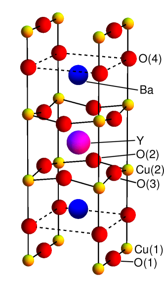
Figure 8: The crystal structure found within the molecular dynamics procedure calculated for a single unit cell with fixed lattice parameters $a=3.82$ Å, $b=3.89$ Å, and $c=11.68$ Å.

To construct a GB with well defined misalignment angle we have to fix the atomic positions on both sides of the interface. In addition we apply periodic boundary conditions in the molecular dynamics procedure in the directions parallel to the GB plane. In the direction perpendicular to the GB only atoms with a distance from the GB plane smaller than 6 lattice constants are reconstructed.

Since we are only interested in deriving stable equilibrium positions for all atoms in the GB region and do not try to simulate the temperature dependent dynamics of the system we completely remove the kinetic energy at the end of every iteration step. With this method the ions relax to their equilibrium positions following paths given by classical forces. With this procedure we are very likely to end up with an ionic distribution that corresponds to a local minimum of the potential energy instead of reaching the true ground state of the system. Randomly changing the initial setup of the GB before starting the reconstruction we are thus able to find different GB structures corresponding to the same misalignment angle $\alpha$. This reflects the experimental situation where one also observes different patterns of ionic arrangements along a macroscopic grain boundary with fixed misalignment angle. For all GB angles under consideration (except the 710 GB) we have reconstructed and analyzed two differently reconstructed grain boundary structures. An example of a reconstructed 410 GB is shown in Fig. 7 c). Finally we can identify the charateristic structural units as classified in Ref. Pennycook, . Here we distinguish between structural units of the bulk material and structural units that are formed due to the lattice mismatch at the GB. The first group consists of (deformed) rectangular and triangular units, that can be seen as fragments of a full rectangular unit, while the latter group consists of large pentagonal units bordered by either Cu or Y ions, that introduce strong deformations and can be identified as the centres of classical dislocation cores (see Fig. 7 d).

Appendix B The effective tight-binding model Hamiltonian

B.1 Slater-Koster method for the calculation of hopping matrix elements

In the following we will derive a tight-binding Hamiltonian for the CuO₂ planes with charge carriers located in the $d_{x^{2}-y^{2}}$ orbitals of the copper atoms. The kinetic energy associated with the hopping of charge carriers from one Cu site to one of its neighboring sites can be calculated from the orbital overlaps of two Cu-$d$ orbitals. Besides the direct overlap between two Cu-$d$ orbitals, that is small due to the small spatial extension of the Cu-$3d$ orbitals, we will also include the indirect hopping “bridged” by an O-$p$ orbital, that can be calculated in second order perturbation theory. Here we will have to add up all possible second order processes involving the O-$p_{x}$ and O-$p_{y}$ orbitals of all intermediate oxygen atoms. In the vicinity of the grain boundary, the directional dependences of the orbital overlaps become important and we calculate the interatomic hopping elements from the Slater and Koster table of the displacement dependent interatomic matrix elements SlaterKoster ; Harrison that depend on the direction cosines $l$, $m$ and $n$ of the vector pointing from one atom to the next, $\vec{r}=(l\vec{e}_{x}+m\vec{e}_{y}+n\vec{e}_{z})d$. In addition, we calculate the effective potentials $V_{pd\sigma}$ and $V_{pd\pi}$ for the $\sigma$- or $\pi$-bonds between the O-$p$ and the Cu-$d$ orbitals, as well as the potentials $V_{dd\sigma}$ and $V_{dd\delta}$ for the $\sigma$- or $\delta$-bonds between two Cu-$d$ orbitals using the effective parameters provided in Ref. Harrison, . In the following we will outline the calculational scheme used within this work by deriving the effective hopping parameter between two neighboring Cu ions in a bulk configuration of a flat CuO₂ plane with an average Cu-O distance of

$$d_{\textrm{Cu-O}}=1.95\textrm{\AA}=3.685a_{0}.$$

As a first step we calculate the hopping between the Cu-$d_{x^{2}-y^{2}}$ orbital and the O-$p_{x}$ orbital that are connected by the vector $\vec{r}=d\vec{e}_{x}$ and therefore $l=1$ and $m=n=0$. The angular dependence is introduced as

$$E_{x,x^{2}-y^{2}}=\frac{1}{2}3^{1/2}l(l^{2}-m^{2})V_{pd\sigma}+l(1-l^{2}+m^{2})V_{pd\pi}=\frac{1}{2}3^{1/2}V_{pd\sigma}.$$

In the next step we have to calcuate the distance-dependent potential of the $\sigma$-bond

$$V_{pd\sigma}=\eta_{pd\sigma}\frac{\hbar^{2}r_{d}^{3/2}}{md^{7/2}}=-2.95\cdot 7.62\textrm{ eV \AA${}^{2}$}\frac{(0.67\textrm{\AA})^{3/2}}{(1.95\textrm{\AA})^{7/2}}=-1.19061\textrm{ eV},$$

where we have used $\frac{\hbar^{2}}{m}=7.62$ eV Ų  and the characteristic length $r_{d}=0.67$ Å  of the Cu-$d$ orbital has been taken from Ref. Harrison, . Now we can calculate the interatomic matrix element as

$$E_{x,x^{2}-y^{2}}=\frac{1}{2}3^{1/2}V_{pd\sigma}=-1.0311\textrm{ eV}.$$

The corresponding hopping parameter between the Cu-$d$ and the O-$p_{y}$ orbital vanishes due to a basic symmetry argument. The directional part of the direct overlap between two Cu-$d$ orbitals on nearest neighbor Cu sites ($d_{\textrm{Cu-Cu}}=3.9$ Å) can be calculated as

$$E_{x^{2}-y^{2},x^{2}-y^{2}}=\frac{3}{4}V_{dd\sigma}+\frac{1}{4}V_{dd\delta}=\frac{3}{4}V_{dd\sigma}.$$

Again we need in addition the distance-dependent potential of the $\sigma$-bond of two Cu-$d$ orbitals:

$$V_{dd\sigma}=\eta_{dd\sigma}\frac{\hbar^{2}r_{d}^{3}}{md^{5}}=-16.2\cdot 7.62\textrm{ eV}\textrm{\AA}^{2}\cdot\frac{(0.67\textrm{\AA})^{3}}{(3.9\textrm{\AA})^{5}}=-0.04115\textrm{ eV},$$

and the total energy associated with the direct overlap of two Cu-$d$ orbitals can finally be calculated as

$$E_{x^{2}-y^{2},x^{2}-y^{2}}=\frac{3}{4}V_{dd\sigma}=-0.03086\textrm{ eV}.$$

Now we can compare this energy to the kinetic energy describing the superexchange between two Cu sites via the O-$p$ orbitals

$$E_{\textrm{Cu-Cu}}=\frac{E_{x,x^{2}-y^{2}}\cdot E_{x,x^{2}-y^{2}}}{\epsilon_{d}-\epsilon_{p}}+\frac{E_{y,x^{2}-y^{2}}\cdot E_{y,x^{2}-y^{2}}}{\epsilon_{d}-\epsilon_{p}}=\frac{1.06317}{-3.5}\textrm{ eV}+0\textrm{ eV}=-0.304\textrm{ eV}.$$

Due to a strong renormalization of the site energies in the cuprates the effective charge transfer gap $\Delta=\epsilon_{p}-\epsilon_{d}$ is larger than one would expect from the difference of the bare site energies of the Cu-$3d$ and the O-$2p$ orbitals Alloul . Here we have chosen the charge transfer gap to be $\Delta=3.5$ eV, a value that is consistent with the range of values found in numerical studies. The full matrix element between two Cu-$d$ orbitals is now the sum of the direct overlap and the second order term including the intermediate O-$p$ orbitals.

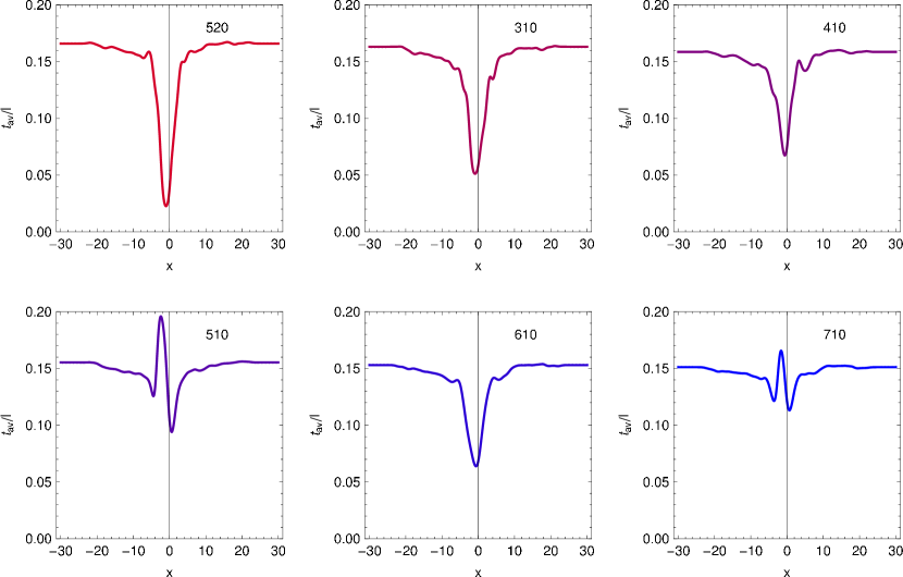
Figure 9: The averaged hopping as a function of the distance to the GB plane for different GBs.

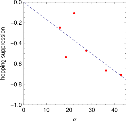
Figure 10: The suppression of the hopping as a function of the misalignment angle $\alpha$ (red points) and a linear fit (blue dashed line). The hopping suppression is defined as the intgral over a Gaussian fit of the hopping profiles shown in Fig. 9.

In Fig. 9 we show the averaged hopping as a function of the distance to the grain boundary plane for different GBs. If we fit the suppressed hopping values in the vicinity of the grain boundary by a Gaussian form and integrate over the “effective barrier” derived in this way, we find only a linear variation with misalignment angle (see Fig. 10).

B.2 The bond valence analysis

The structural imperfection at the grain boundary will necessarily lead to charge inhomogeneities that will contribute — in a similar way as the reduced hopping — to the effective barrier that blocks the superconducting current over the GB. We can include these charge inhomogeneities in our calculations by “translating” them into on-site potentials on the Cu sites. It is evident that we also have to include the charges on the O sites in our considerations although the O sites themselves have already been integrated out in the effective one-band tight-binding model. We will start our considerations by assigning every atom of the perfect crystal a formal integer ionic charge: Y³⁺, Ba²⁺, O^2-. The requirement of charge neutrality leaves us with 7 positive charges to be distributed on the 3 Cu atoms: Thus we will have two Cu²⁺, and one Cu³⁺ ion per unit cell. For a crystal with bonds that are neither strictly covalent nor strictly ionic it is convenient to introduce a fractional valence for each ion, that is determined with respect to its ionic environment in the unit cell of the crystal. Here we calculate the bond valence of a cation by

$$V_{i}=\sum_{j}\exp\left(\frac{r_{0}-r_{ij}}{B}\right),$$

where the sum is over all neighboring anions, in our case the neighboring negatively charged O and $r_{ij}$ is the cation-anion distance. Here we take $B=0.37$ Å  following Ref. Brown, , while $r_{0}$ is different for all cation-anion pairs and can also depend on the formal integer oxidation state of the ion. The basic idea is that the bond valence sum should agree with the assumed integer oxidation state of the ion, and strong deviations indicate strain in the crystal or even an incorrect structure. This seems to be a very clear concept for the case of the Y³⁺ and Ba²⁺ ions. For the copper atoms, where we can have more than one formal integer oxidation state, the situation is slightly more complicated. Following Refs. Brown, ; Chmaissem, we define $\xi_{i}^{(3)}$ as the fraction of Cu ions at site $i$ that are in a Cu³⁺-type oxidation state while the remaining $(1-\xi_{i}^{(3)})$ Cu ions are in a Cu²⁺-type oxidation state. With this the average oxidation state of the Cu ion at site $i$ is

$$\bar{V}_{i}=3\xi_{i}^{(3)}+2(1-\xi_{i}^{(3)})=2+\xi_{i}^{(3)}.$$

On the other hand, this should be equal to the sum of a fraction of bond valences $V_{i}^{(3+)}$ of ions characterized by $r_{0}(\textrm{Cu}^{3+})=1.73$ Å  and a fraction of bond valences $V_{i}^{(2+)}$ of ions characterized by $r_{0}(\textrm{Cu}^{2+})=1.679$ Å:

$$\bar{V}_{i}=\xi_{i}^{(3)}V_{i}^{(3+)}+(1-\xi_{i}^{(3)})V_{i}^{(2+)}.$$

Solving this set of equations for $\xi_{i}^{(3)}$ allows us to determine the fraction of Cu ions with the valence $3+$:

$$\xi_{i}^{(3)}=\frac{V_{i}^{(2+)}-2}{V_{i}^{(2+)}-V_{i}^{(3+)}+1}.$$

In a similar way we can proceed assuming that we have a Cu ion that could be in a 1+ or a 2+ oxidation state. Here we will use $r_{0}(\textrm{Cu}^{2+})=1.679$ Å  and $r_{0}(\textrm{Cu}^{1+})=1.6$ Å  and we find

$$\xi_{i}^{(1)}=\frac{V_{i}^{(2+)}-2}{V_{i}^{(2+)}-V_{i}^{(1+)}-1}.$$

In the case that Cu²⁺ and Cu³⁺ are the most probable oxidation states we will find that $\xi_{i}^{(3)}$ is positive and $\xi_{i}^{(1)}$ is negative while in the case that Cu²⁺ and Cu⁺ are the most probable oxidation states we will find that $\xi_{i}^{(1)}$ is positive and $\xi_{i}^{(3)}$ is negative. For the calculation of the final oxidation state of a particular Cu atom one has to use the correct, positive $\xi_{i}$.

In a last step we determine the fractional valence of the O ions by summing up all charge contributions from the neighboring cations. Here we assume that the Ba and the Y ions are in their formal integer oxidations state whereas we assign every Cu ion a fractional oxidation state determined by $\xi_{i}^{(1/3)}$. This method ensures that we end up with a charge neutral crystal.

In the bulk system we derive fractional valences close to the formal integer oxidation states. In the vicinity of the GB we find however deviations from the bulk values due to missing or displaced neighboring ions.

B.3 The definition of the superconducting pairing interaction

To model the known momentum space structure of the superconducting order parameter in the weak coupling description of the Bogoliubov-de Gennes theory, one usually defines an interaction $V_{ij}$ on the bonds connecting two nearest neighbor Cu sites. Unfortunately, there is no obvious way to define an analogous pairing interaction in a strongly disordered region of the crystal, as e.g. in the vicinity of the GB, since the exact microscopic origin of this interaction is not known. Assuming that a missing or a broken Cu-O bond destroys the underlying pairing mechanism, we develop a method of tying the superconducting pairing interaction between two Cu sites to the hopping matrix elements connecting the two sites as well as to the charge imbalance between them. Hence we define the pairing interaction on a given bond as the product of a dimensionless constant $V_{0}$, that is adjusted to reproduce the correct modulus of the gap in the bulk, and the hopping parameter $t_{ij}$. In addition we impose an exponential suppression of the pairing strength with increasing charge imbalance:

$$V_{ij}=V_{0}t_{ij}e^{-|Q_{i}-Q_{j}|/e}.$$

To avoid long range contributions to the pairing we use a threshhold of $0.2$ eV for $|t_{ij}|$, thus restricting the pairing interaction to the bonds between nearest neighbor Cu sites in the bulk. Here we emphasize that although we tried to model the pairing interaction in a realistic way, the exact procedure how we define the pairing interaction in the disordered region does not qualitatively change the results.

Appendix C The calculation of the critical current

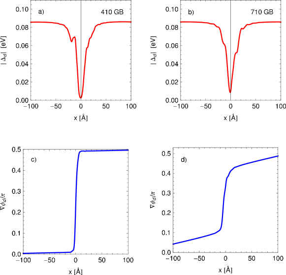
Figure 11: The modulus (a,b) and the phase (c,d) of the self-consistently calculated order parameter as a function of the distance to the GB plane for a 410 and for a 710 GB.

The superconducting current over a weak link, as well as over a metallic or an insulating barrier is accompanied by a drastic change of the phase of the superconducting order parameter. For a true tunnel junction, for which the two superconducting regions are completely decoupled, the current-phase relation is known to be sinusoidal, and the maximum current is found for a phase jump of $\pi/2$. For a weak link, as e.g. provided by a geometrical constriction or a disordered region like a grain boundary, the phase of the superconducting order parameter has to change continously between its two bulk values in the leads on both sides of the weak link. Here one would expect deviations from the sinusoidal current-phase relation and a smooth transition of the phase over a length scale given by the dimensions of the weak link. Besides the change in the phase of the order parameter in the presence of an applied current, a weak link is also characterized by a suppression of the modulus of the order parameter, either due to geometric restrictions or due to strong disorder. An additional suppression of the order parameter on the length scale of the coherence length can occur due to the formation of Andreev bound states present at specifically orientated interfaces of $d$-wave superconductors. Here we have calculated the order parameter self-consistently from Eq. 8 in the main text and found a suppression of its modulus in the vicinity of the grain boundary that depends in its width and depth only weakly on the misalignment angle (compare Fig. 11 a,b).

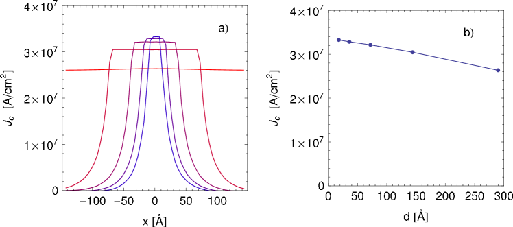
Figure 12: (a) The current profile as a function of the distance $x$ to the GB plane for a 710 GB. The phase of the order parameter has been fixed at different distances $d/2$ from the GB. (b) The dependence of the critical current as a function of the distance $d$ between the two points at which the phase of the order parameter has been fixed.

For a numerical determination of the critical current — the maximum current that can be applied to a system without destroying its superconducting properties — it is convenient to enforce a certain phase difference of the order parameter between two points of the system separated by a distance $d$, e.g. in our example on both sides of the grain boundary region. Here we calculate the superconducting current over the grain boundary modelled by the Hamiltonian in Eq. 5 of the main text using Eqs. 9 and 10 therein and fixing the phase of the order parameter in the leads in every iteration step. The critical current for our system can then be found as the current maximum under a variation of the phase difference. If a strong perturbation limits the superconducting current — in the so-called tunneling limit — the main drop of the superconducting phase will appear in the small region of the perturbation and the change of the phase in the superconducting leads is negligible (see Fig. 11 c). However, if the perturbation is weak, the change of the phase in the superconducting leads becomes more important (see Fig. 11 d) and the current will depend on the distance $d$ between the two points, at which the phase of the order parameter is fixed. Since we are interested in the calculation of the critical current, we have to decrease the distance, thus increasing the phase gradient, until we reach the maximum current. To calculate the current over the low angle grain boundaries, we have determined the maximum current by extrapolating it to the value expected for $d=0$ (see Fig. 12).