Abstract

Setting up an empirical model of optical sensing to exploit the circular Bragg phenomenon displayed by chiral sculptured thin films (CSTFs), we considered a CSTF with and without a central twist defect of $\pi/2$ radians. The circular Bragg phenomenon of the defect-free CSTF, and the spectral hole in the co-polarized reflectance spectrum of the CSTF with the twist defect, were both found to be acutely sensitive to the refractive index of a fluid which infiltrates the void regions of the CSTF. These findings bode well for the deployment of CSTFs as optical sensors.

1 Introduction

By means of physical vapor deposition, an array of parallel helical nanowires—known as a chiral sculptured thin film (CSTF)—may be grown on a substrate [1, 2]. At optical wavelengths, a CSTF may be regarded as a unidirectionally nonhomogeneous continuum. CSTFs display orthorhombic symmetry locally whereas they are structurally chiral from a global perspective [3, Chap. 9]. There are two key attributes which render CSTFs attractive for a host of applications. Firstly, CSTFs exhibit the circular Bragg phenomenon (just as cholesteric liquid crystals do [4]). Thus, a structurally right/left-handed CSTF of sufficient thickness almost completely reflects right/left-circularly polarized (RCP/LCP) light which is normally incident, but normally incident LCP/RCP light is reflected very little, when the free-space wavelength lies within the Bragg regime. This property has led to the use of CSTFs as circular polarization [5], spectral-hole [6], and S̆olc [7] filters, among other applications [8, 9]. Secondly, CSTFs are porous, and their multiscale porosity can be tailored to allow only species of certain shapes and sizes to infiltrate their void regions [10]. This engineered porosity, combined with the circular Bragg phenomenon, makes CSTFs attractive as platforms for light-emitting devices with precise control over the circular polarization state and the emission wavelengths [11, 12], and optical biosensors [13, 14].

Further possibilities for a CSTF emerge if a structural twist defect is introduced. For example, if the upper half of a CSTF is twisted by $\pi/2$ radians about the axis of nonhomogeneity relative to the lower half, then the co-polarized reflectance spectrum contains a spectral hole in the middle of the Bragg regime [15, 16]. This phenomenon may be exploited for narrow-bandpass filtering [17], as well as for optical sensing of fluids which infiltrate the void regions of the CSTF [18, 19].

We devised an empirical model yielding the sensitivity of a CSTF’s optical response—as a circular Bragg filter—to the refractive index of a fluid which infiltrates the CSTF’s void regions, with a view to optical-sensing applications. We considered both a defect-free CSTF and a CSTF with a central $\pi/2$-twist defect. Our model is not limited to normal incidence but also encompasses oblique incidence, and we present computed results for slightly off-normal incidence, a realistic situation for sensing applications. Furthermore, because the material that is deposited as the CSTF is not precisely the same as the bulk material that is evaporated, we use an inverse homogenization procedure [20] on related but uninfiltrated columnar thin films (CTFs) [21] to predict the spectral shifts due to infiltration of CSTFs.

An $\exp(-i\omega t)$ time-dependence is implicit, with $\omega$ denoting the angular frequency and $i=\sqrt{-1}$. The free-space wavenumber, the free-space wavelength, and the intrinsic impedance of free space are denoted by $k_{0}=\omega\sqrt{\epsilon_{0}\mu_{0}}$, $\lambda_{0}=2\pi/k_{0}$, and $\eta_{0}=\sqrt{\mu_{0}/\epsilon_{0}}$, respectively, with $\mu_{0}$ and $\epsilon_{0}$ being the permeability and permittivity of free space. Vectors are in boldface, dyadics are underlined twice, column vectors are in boldface and enclosed within square brackets, and matrixes are underlined twice and square-bracketed. The Cartesian unit vectors are identified as ${{\bf u}}_{x}$, ${{\bf u}}_{y}$, and ${{\bf u}}_{z}$.

2 Empirical Model

2.1 Uninfiltrated defect-free CSTF

Let us begin the explication of our empirical model with a defect-free CSTF with vacuous void regions; i.e., an uninfiltrated CSTF. The $z$ direction is taken to be the direction of nonhomogeneity. The CSTF is supposed to have been grown on a planar substrate through the deposition of an evaporated bulk material [3]. The substrate, which lies parallel to the plane $z=0$, is supposed to have been rotated about the $z$ axis at a uniform angular speed throughout the deposition process. The rise angle of each resulting helical nanowire, relative to the $xy$ plane, is denoted by $\chi$. The refractive index of the deposited material — assumed to be an isotropic dielectric material — is written as $n_{s}$, which can be different from the refractive index of the bulk material that was evaporated [22, 23, 24].

Each nanowire of a CSTF can be modeled as a string of highly elongated ellipsoidal inclusions, wound end-to-end around the $z$ axis to create a helix [25, 26]. The surface of each ellipsoidal inclusion is characterized by the shape dyadic

$${{\bf u}}_{n}\,{{\bf u}}_{n}+\gamma_{\tau}\,{{\bf u}}_{\tau}\,{{\bf u}}_{\tau}+\gamma_{b}\,{{\bf u}}_{b}\,{{\bf u}}_{b},$$ (1)

wherein the normal, tangential and binormal basis vectors are given as

$$\left.\begin{array}[]{l}{{\bf u}}_{n}=-{{\bf u}}_{x}\,\sin\chi+{{\bf u}}_{z}\,\cos\chi\vspace{4pt}\\ {{\bf u}}_{\tau}={{\bf u}}_{x}\,\cos\chi+{{\bf u}}_{z}\,\sin\chi\vspace{4pt}\\ {{\bf u}}_{b}=-{{\bf u}}_{y}\end{array}\right\}.$$ (2)

By choosing the shape parameters $\gamma_{b}\gtrsim 1$ and $\gamma_{\tau}\gg 1$, an aciculate shape is imposed on the inclusions. For the numerical results presented in §3, we fixed $\gamma_{\tau}=15$ while noting that increasing $\gamma_{\tau}$ beyond 10 does not give rise to significant effects for slender inclusions [26]. The helical nanowires occupy only a proportion $f\in\left(0,1\right)$ of the total CSTF volume; the volume fraction of the CSTF not occupied by nanowires is $1-f$.

At length scales much greater than the nanoscale, the CSTF’s relative permittivity dyadic may be expressed as

$$\underline{\underline{\epsilon}}_{\,1}={\underline{\underline{S}}}_{\,z}\left(h\frac{\pi z}{\Omega}\right)\mbox{ \tiny{${}^{\bullet}$} }{\underline{\underline{S}}}_{\,y}\left(\chi\right)\mbox{ \tiny{${}^{\bullet}$} }\underline{\underline{\epsilon}}^{ref}_{\,1}\mbox{ \tiny{${}^{\bullet}$} }{\underline{\underline{S}}}^{T}_{\,y}\left(\chi\right)\mbox{ \tiny{${}^{\bullet}$} }{\underline{\underline{S}}}^{T}_{\,z}\left(h\frac{\pi z}{\Omega}\right),$$ (3)

where $2\Omega$ is the structural period and the rotation dyadics

$$\left.\begin{array}[]{l}{\underline{\underline{S}}}_{\,y}\left(\chi\right)={\bf u}_{y}\,{\bf u}_{y}+\left({\bf u}_{x}\,{\bf u}_{x}+{\bf u}_{z}\,{\bf u}_{z}\right)\cos\chi+\left({\bf u}_{z}\,{\bf u}_{x}-{\bf u}_{x}\,{\bf u}_{z}\right)\sin\chi\vspace{4pt}\\ {\underline{\underline{S}}}_{\,z}\left(\sigma\right)={\bf u}_{z}\,{\bf u}_{z}+\left({\bf u}_{x}\,{\bf u}_{x}+{\bf u}_{y}\,{\bf u}_{y}\right)\cos\sigma+\left({\bf u}_{y}\,{\bf u}_{x}-{\bf u}_{x}\,{\bf u}_{y}\right)\sin\sigma\end{array}\right\}.$$ (4)

The handedness parameter $h=+1$ for a structurally right-handed CSTF, and $h=-1$ for a structurally left-handed CSTF. The reference relative permittivity dyadic $\underline{\underline{\epsilon}}^{ref}_{\,1}$ has the orthorhombic form

$$\underline{\underline{\epsilon}}^{ref}_{\,1}=\epsilon_{a1}\,{{\bf u}}_{n}\,{{\bf u}}_{n}+\epsilon_{b1}\,{{\bf u}}_{\tau}\,{{\bf u}}_{\tau}\,+\,\epsilon_{c1}\,{{\bf u}}_{b}\,{{\bf u}}_{b}.$$ (5)

The nanowire rise angle $\chi$ can be measured from scanning-electron-microscope imagery. In principle, the relative permittivity parameters $\left\{\epsilon_{a1},\epsilon_{b1},\epsilon_{c1}\right\}$ of an uninfiltrated CSTF are also measurable. However, in view of the paucity of suitable experimental data on CSTFs, our empirical model relies on the measured experimental data on the related columnar thin films (CTFs). In order to deposit both CSTFs and CTFs, the vapor flux is directed at a fixed angle $\chi_{v}$ with respect to the substrate plane. The different morphologies of CSTFs and CTFs are due to the rotation of the substrate for the former but not for the latter. The parameters $\left\{\epsilon_{a1},\epsilon_{b1},\epsilon_{c1},\chi\right\}$ are functions of $\chi_{v}$.

The nanoscale model parameters $\left\{n_{s},f,\gamma_{b}\right\}$ are not readily determined by experimental means. However, the process of inverse homogenization can be employed to determine these parameters from a knowledge of $\left\{\epsilon_{a1},\epsilon_{b1},\epsilon_{c1}\right\}$, as was done for titanium-oxide CTFs in a predecessor paper [20].

2.2 Infiltrated defect-free CSTF

With optical-sensing applications in mind, next we consider the effect of filling the void regions of a defect-free CSTF with a fluid of refractive index $n_{\ell}$. This brings about a change in the reference relativity permittivity dyadic. The infiltrated CSTF is characterized by the relative permittivity dyadic $\underline{\underline{\epsilon}}_{\,2}$, which has the same eigenvectors as $\underline{\underline{\epsilon}}_{\,1}$ but different eigenvalues. Thus, the infiltrated CSTF is characterized by (3) and (5), but with $\underline{\underline{\epsilon}}_{\,2}$ in lieu of $\underline{\underline{\epsilon}}_{\,1}$, $\underline{\underline{\epsilon}}^{ref}_{\,2}$ in lieu of $\underline{\underline{\epsilon}}^{ref}_{\,1}$ and $\left\{\epsilon_{a2},\epsilon_{b2},\epsilon_{c2}\right\}$ in lieu of $\left\{\epsilon_{a1},\epsilon_{b1},\epsilon_{c1}\right\}$. The nanowire rise angle $\chi$ remains unchanged.

In our model, the Bruggeman homogenization formalism is applied in its usual forward sense [27] to determine $\left\{\epsilon_{a2},\epsilon_{b2},\epsilon_{c2}\right\}$, from knowledge of the nanoscale model parameters $\left\{n_{s},f,\gamma_{b}\right\}$ together with $\left\{n_{\ell},\gamma_{\tau}\right\}$, as described elsewhere [26].

2.3 Boundary-value problem

Let us now suppose that a CSTF occupies the region $0\leq z\leq L$, with the half-spaces $z<0$ and $z>L$ being vacuous. An arbitrarily polarized plane wave is incident on the CSTF from the half-space $z<0$. Its wavevector lies in the $xz$ plane, making an angle $\theta\in\left[0,\pi/2\right)$ relative to the $+z$ axis. As a result, there is a reflected plane wave in the half-space $z<0$ and a transmitted plane wave in the half-space $z>L$. Thus, the total electric field phasor in the half-space $z<0$ may be expressed as

$${\bf E}({\bf r}) = \left[a_{L}\frac{i{\bf u}_{y}-{\bf p}_{+}}{\sqrt{2}}-a_{R}\frac{i{\bf u}_{y}+{\bf p}_{+}}{\sqrt{2}}\right]\,\exp\left({i\kappa}x\right)\,\exp\left(ik_{0}z\cos\theta\right)$$ (6)

$$\quad-\left[r_{L}\frac{i{\bf u}_{y}-{\bf p}_{-}}{\sqrt{2}}-r_{R}\frac{i{\bf u}_{y}+{\bf p}_{-}}{\sqrt{2}}\right]\,\exp\left({i\kappa}x\right)\,\exp\left(-ik_{0}z\cos\theta\right),\quad z<0,$$

while that in the half-space $z>L$ may be expressed as

$${\bf E}({\bf r})=\left[t_{L}\frac{i{\bf u}_{y}-{\bf p}_{+}}{\sqrt{2}}-t_{R}\frac{i{\bf u}_{y}+{\bf p}_{+}}{\sqrt{2}}\right]\,\exp\left({i\kappa}x\right)\,\exp\left[ik_{0}\left(z-L\right)\cos\theta\right],\quad z>L,$$ (7)

wherein ${\bf p}_{\pm}=\mp{\bf u}_{x}\cos\theta+{\bf u}_{z}\sin\theta$ and $\kappa=k_{0}\sin\theta$.

Our aim is to determine the unknown amplitudes $r_{L}$ and $r_{R}$ of the LCP and RCP components of the reflected plane wave, and the unknown amplitudes $t_{L}$ and $t_{R}$ of the LCP and RCP components of the transmitted plane wave, from the known amplitudes $a_{L}$ and $a_{R}$ of the LCP and RCP components of the incident plane wave. As is comprehensively described elsewhere [3], this is achieved by solving the 4$\times$4 matrix/4-vector relation

$$[{\bf f}^{exit}]=[\underline{\underline{M}}(L)]\mbox{ \tiny{${}^{\bullet}$} }[{\bf f}^{entry}].$$ (8)

Here, the column 4-vectors

$$[{\bf f}^{entry}]=\frac{1}{\sqrt{2}}\left(\begin{array}[]{c}\left(r_{L}+rR\right)+\left(a_{L}+a_{R}\right)\vspace{4pt}\\ i\left[-\left(r_{L}-rR\right)+\left(a_{L}-a_{R}\right)\right]\vspace{4pt}\\ -i\left[\left(r_{L}-rR\right)+\left(a_{L}-a_{R}\right)\right]/\eta_{0}\vspace{4pt}\\ -\left[\left(r_{L}+rR\right)-\left(a_{L}+a_{R}\right)\right]/\eta_{0}\end{array}\right),\quad[{\bf f}^{exit}]=\frac{1}{\sqrt{2}}\left(\begin{array}[]{c}t_{L}+tR\vspace{4pt}\\ i\left(t_{L}-tR\right)\vspace{4pt}\\ -i\left(t_{L}-tR\right)/\eta_{0}\vspace{4pt}\\ \left(t_{L}+tR\right)/\eta_{0}\end{array}\right),$$ (9)

arise from the field phasors at $z=0$ and $z=L$, respectively. The optical response characteristics of the CSTF are encapsulated by the 4$\times$4 transfer matrix $[\underline{\underline{M}}(L)]$, which is conveniently expressed as [28]

$$[\underline{\underline{M}}(L)]=[\underline{\underline{B}}(h\frac{\pi z}{\Omega})]\mbox{ \tiny{${}^{\bullet}$} }[\underline{\underline{M}}^{\prime}(L)],$$ (10)

wherein the 4$\times$4 matrix

$$[\underline{\underline{B}}(\sigma)]=\left(\begin{array}[]{cccc}\cos\sigma&-\sin\sigma&0&0\\ \sin\sigma&\cos\sigma&0&0\\ 0&0&\cos\sigma&-\sin\sigma\\ 0&0&\sin\sigma&\cos\sigma\end{array}\right).$$ (11)

The 4$\times$4 matrizant $[\underline{\underline{M}}^{\prime}(z)]$ satisfies the ordinary differential equation

$$\frac{d}{dz}[\underline{\underline{M}}^{\prime}(z)]=i\,[\underline{\underline{P}}^{\prime}(z)]\mbox{ \tiny{${}^{\bullet}$} }[\underline{\underline{M}}^{\prime}(z)],$$ (12)

subject to the boundary condition $[\underline{\underline{M}}^{\prime}(0)]=[\underline{\underline{I}}]$, with $[\underline{\underline{I}}]$ being the identity 4$\times$4 matrix. The 4$\times$4 matrix [28]

$$[\underline{\underline{P}}^{\prime}(z)]=\begin{bmatrix}0&-ih\frac{\pi}{\Omega}&0&\omega\mu_{0}\\ ih\frac{\pi}{\Omega}&0&-\omega\mu_{0}&0\\ 0&-\omega\epsilon_{0}\epsilon_{\rm c}&0&-ih\frac{\pi}{\Omega}\\ \frac{\omega\epsilon_{0}\epsilon_{b}}{\tau}&0&ih\frac{\pi}{\Omega}&0\end{bmatrix}\,+$$

$$\begin{bmatrix}-\frac{\kappa\left(\epsilon_{b}-\epsilon_{a}\right)}{2\epsilon_{a}\tau}\cos\xi\sin{2\chi}&0&-\frac{\kappa^{2}}{\omega\epsilon_{0}\epsilon_{a}\tau}\sin\xi\cos\xi&-\frac{\kappa^{2}}{\omega\epsilon_{0}\epsilon_{a}\tau}\cos^{2}\xi\\ &&&\\ \frac{\kappa\left(\epsilon_{b}-\epsilon_{a}\right)}{2\epsilon_{a}\tau}\sin\xi\sin{2\chi}&0&\frac{\kappa^{2}}{\omega\epsilon_{0}\epsilon_{a}\tau}\sin^{2}\xi&\frac{\kappa^{2}}{\omega\epsilon_{0}\epsilon_{a}\tau}\sin\xi\cos\xi\\ &&&\\ \frac{\kappa^{2}}{\omega\mu_{0}}\sin\xi\cos\xi&\frac{\kappa^{2}}{\omega\mu_{0}}\cos^{2}\xi&0&0\\ &&&\\ -\frac{\kappa^{2}}{\omega\mu_{0}}\sin^{2}\xi&-\frac{\kappa^{2}}{\omega\mu_{0}}\sin\xi\cos\xi&-\frac{\kappa\left(\epsilon_{b}-\epsilon_{a}\right)}{2\epsilon_{a}\tau}\sin\xi\sin{2\chi}&-\frac{\kappa\left(\epsilon_{b}-\epsilon_{a}\right)}{2\epsilon_{a}\tau}\cos\xi\sin{2\chi}\end{bmatrix}\,$$ (13)

containing

$$\xi=h\pi z/\Omega,\qquad\tau=\cos^{2}\chi+\left(\epsilon_{b}/\epsilon_{a}\right)\sin^{2}\chi$$ (14)

depends on whether the CSTF is uninfiltrated or infiltrated. Equation (12) can be solved for $[\underline{\underline{M}}^{\prime}(z)]$ by numerical means, most conveniently using a piecewise uniform approximation [3].

Once $[\underline{\underline{M}}^{\prime}(z)]$ is determined, it is a straightforward matter of linear algebra to extract the reflection amplitudes $r_{L,R}$ and transmission amplitudes $t_{L,R}$ from (8), for specified incident amplitudes $a_{L,R}$. Following the standard convention, we introduce the reflection coefficients $r_{LL,LR,RL,RR}$ and transmission coefficients $t_{LL,LR,RL,RR}$ per

$$\left(\begin{array}[]{c}r_{L}\vspace{4pt}\\ r_{R}\end{array}\right)=\left(\begin{array}[]{cc}r_{LL}&r_{LR}\vspace{4pt}\\ r_{RL}&r_{RR}\end{array}\right)\left(\begin{array}[]{c}a_{L}\vspace{4pt}\\ a_{R}\end{array}\right),\qquad\quad\left(\begin{array}[]{c}t_{L}\vspace{4pt}\\ t_{R}\end{array}\right)=\left(\begin{array}[]{cc}t_{LL}&t_{LR}\vspace{4pt}\\ t_{RL}&t_{RR}\end{array}\right)\left(\begin{array}[]{c}a_{L}\vspace{4pt}\\ a_{R}\end{array}\right).$$ (15)

The square magnitude of a reflection or transmission coefficient yields the corresponding reflectance or transmittance; i.e., $R_{\alpha\beta}=\left|r_{\alpha\beta}\right|^{2}$ and $T_{\alpha\beta}=\left|t_{\alpha\beta}\right|^{2}$, where $\alpha,\beta\in\left\{L,R\right\}$.

2.4 CSTF with central $\pi/2$-twist defect

As mentioned in §1, the introduction of a central twist defect leads to a narrowband feature that can be very useful for sensing applications. Therefore, we further consider the CSTF of finite thickness introduced in §2.3 but here with the upper half $z\in\left[L/2,L\right]$ of the CSTF twisted about the $z$ axis by an angle of $\pi/2$ radians with respect to the lower half $z\in\left[0,L/2\right)$.

Mathematically, the central $\pi/2$-twist defect is accommodated as follows: The relative permittivity dyadic of the centrally twisted uninfiltrated CSTF is per (3) but with the rotation dyadic ${\underline{\underline{S}}}_{\,z}\left(h\frac{\pi z}{\Omega}\right)$ therein replaced by ${\underline{\underline{S}}}_{\,z}\left\{h\left[\frac{\pi z}{\Omega}+\psi(z)\right]\right\}$, where

$$\psi(z)=\left\{\begin{array}[]{lcr}0,&&0\leq z<L/2\vspace{6pt}\\ \pi/2,&&L/2\leq z\leq L\end{array}\right..$$ (16)

The relative permittivity dyadic of the centrally twisted and infiltrated CSTF follows from the corresponding dyadic for the centrally twisted and uninfiltrated CSTF, in exactly the same way as is the case when the CSTF is defect-free. The calculation of the reflectances and transmittances follows the same path as is described in §2.3 with the exception that (10) therein is replaced by

$$[\underline{\underline{M}}(L)]=[\underline{\underline{B}}\left(h\frac{\pi L}{2\Omega}+\frac{\pi}{2}\right)]\mbox{ \tiny{${}^{\bullet}$} }[\underline{\underline{M}}^{\prime}(L/2)]\mbox{ \tiny{${}^{\bullet}$} }[\underline{\underline{B}}\left(h\frac{\pi L}{2\Omega}-\frac{\pi}{2}\right)]\mbox{ \tiny{${}^{\bullet}$} }[\underline{\underline{M}}^{\prime}(L/2)].$$ (17)

3 Numerical results

In order to illustrate the empirical model, we chose a CSTF of thickness $L=40\Omega$ where the structural half-period $\Omega=185$ nm. The chosen relative permittivity parameters, namely

$$\left.\begin{array}[]{l}\epsilon_{a1}=\displaystyle{\left[1.0443+2.7394\left(\frac{2\chi_{v}}{\pi}\right)-1.3697\left(\frac{2\chi_{v}}{\pi}\right)^{2}\right]^{2}\vspace{6pt}}\\ \epsilon_{b1}=\displaystyle{\left[1.6765+1.5649\left(\frac{2\chi_{v}}{\pi}\right)-0.7825\left(\frac{2\chi_{v}}{\pi}\right)^{2}\right]^{2}\vspace{6pt}}\\ \epsilon_{c1}=\displaystyle{\left[1.3586+2.1109\left(\frac{2\chi_{v}}{\pi}\right)-1.0554\left(\frac{2\chi_{v}}{\pi}\right)^{2}\right]^{2}}\end{array}\right\}$$ (18)

with

$$\chi=\tan^{-1}\left({2.8818}\tan\chi_{v}\right),$$ (19)

emerged from data measured for a CTF made by evaporating patinal${}^{\mbox{\textregistered}}$ titanium oxide [21]. These relations—which came from measurements at $\lambda_{0}=633$ nm—were presumed to be constant over the range of wavelengths considered here. Values for the corresponding nanoscale model parameters $\left\{n_{s},f,\gamma_{b}\right\}$, as computed using the inverse Bruggeman homogenization formalism [20], are provided in Table 1 for the vapor flux angles $\chi_{v}=15^{\circ}$, $30^{\circ}$, and $60^{\circ}$. Furthermore, we set $h=+1$. The angle of incidence $\theta$ was fixed at $10^{\circ}$.

Computed reflectances and transmittances are plotted versus $\lambda_{0}$ in Fig. 1, for the defect-free CSTF for which we set $\chi_{v}=15^{\circ}$. Further computations (not presented here) using other values of $\chi_{v}$ revealed qualitatively similar graphs of reflectances and transmittances versus $\lambda_{0}$. The effects of three values of $n_{\ell}$—namely, $n_{\ell}=1$, $1.3$ and $1.5$—are represented in Fig. 1. The circular Bragg phenomenon is most obviously appreciated as a sharp local maximum in the graphs of $R_{RR}$, with attendant features occurring in the graphs of some other reflectances and transmittances. If $\lambda^{max}_{0}$ denotes the free-space wavelength corresponding to this local maximum, from Fig. 1, we found that $\lambda_{0}^{max}\approx 622$ nm for $n_{\ell}=1$, $\lambda_{0}^{max}\approx 712$ nm for $n_{\ell}=1.3$, and $\lambda_{0}^{max}\approx 768$ nm for $n_{\ell}=1.5$.

Clearly, the circular Bragg phenomenon undergoes a substantial spectral shift as $n_{\ell}$ increases from unity. In order to elucidate further this matter, we focused on the spectral-shift sensitivity $d\lambda^{max}_{0}/dn_{\ell}$. Graphs of $d\lambda^{max}_{0}/dn_{\ell}$ against $\lambda^{max}_{0}$, computed for the range $1<n_{\ell}<1.5$, are presented in Fig. 2. In addition to results for the vapor flux angle $\chi_{v}=15^{\circ}$, results are also plotted in Fig. 2 for $\chi_{v}=30^{\circ}$ and $\chi_{v}=60^{\circ}$. For all vapor flux angles considered and all values of $n_{\ell}\in\left(1,1.5\right)$, the spectral-shift sensitivity $d\lambda^{max}_{0}/dn_{\ell}$ is positive-valued and greater than 118 nm per refractive index unit (RIU). When $\chi_{v}=15^{\circ}$, $d\lambda^{max}_{0}/dn_{\ell}$ generally decreases as $\lambda^{max}_{0}$ increases. A similar trend is exhibited for $\chi_{v}=30^{\circ}$, but $d\lambda^{max}_{0}/dn_{\ell}$ generally increases as $\lambda^{max}_{0}$ increases for $\chi_{v}=60^{\circ}$.

The center wavelength of the circular Bragg regime has been estimated as [29]

$$\lambda_{0}^{Br}\approx\Omega\left(\sqrt{\epsilon_{c2}}+\sqrt{\frac{\epsilon_{a2}\epsilon_{b2}}{\epsilon_{a2}\cos^{2}\chi+\epsilon_{b2}\sin^{2}\chi}}\right)\sqrt{\cos\theta}.$$ (20)

The graphs of $d\lambda^{Br}_{0}/dn_{\ell}$ versus $\lambda^{Br}_{0}$, as provided in Fig. 3 for the vapor flux angles $\chi_{v}=15^{\circ}$, $30^{\circ}$, and $60^{\circ}$, are remarkably similar (but not identical) to the graphs of $d\lambda^{max}_{0}/dn_{\ell}$ versus $\lambda^{max}_{0}$ displayed in Fig. 2. Thus, the center-wavelength formula (20) can yield a convenient estimate of the spectral-shift sensitivity, without having to solve the reflection-transmission problem.

We turn now to the CSTF with a central twist defect of $\pi/2$ radians, as described in §2.4. Graphs of the reflectances and transmittances versus $\lambda_{0}$ for $\chi_{v}=15^{\circ}$ are provided in Fig. 4. As we remarked for the defect-free CSTF, graphs (not presented here) which are qualitatively similar to those presented in Fig. 4 were obtained when other values of the vapor flux angle $\chi_{v}$ were considered. The graphs of Fig. 4 are substantially different to those of Fig. 1: the local maximums in the graphs of $R_{RR}$ in Fig. 1 have been replaced by sharp local minimums in Fig. 4. These local minimums—which represent an ultranarrowband spectral hole—arise at the free-space wavelengths $\lambda^{min}_{0}$ that are approximately the same as the corresponding local maximums $\lambda^{max}_{0}$ in Fig. 1.

The location of the spectral hole on the $\lambda_{0}$ axis is highly sensitive to $n_{\ell}$. In a similar manner to before, we explore this matter by computing the spectral-shift sensitivity $d\lambda^{min}_{0}/dn_{\ell}$ at each value of $n_{\ell}$. In Fig. 5, $d\lambda^{min}_{0}/dn_{\ell}$ is plotted against $\lambda^{min}_{0}$, with the spectral-shift sensitivity computed for the range $1<n_{\ell}<1.5$ and with $\chi_{v}=15^{\circ}$, $30^{\circ}$, and $60^{\circ}$. The plots of $d\lambda^{min}_{0}/dn_{\ell}$ versus $\lambda^{min}_{0}$ in Fig. 5 are both qualitatively and quantitatively similar to those of $d\lambda^{max}_{0}/dn_{\ell}$ versus $\lambda^{max}_{0}$ in Fig. 2. That is, positive-valued $d\lambda^{min}_{0}/dn_{\ell}$ generally decreases as $\lambda^{min}_{0}$ increases for $\chi_{v}=15^{\circ}$ and $30^{\circ}$, and generally increases as $\lambda^{min}_{0}$ increases for $\chi_{v}=60^{\circ}$. A similar correspondence exists with Fig. 3.

4 Closing remarks

Our empirical model has demonstrated that the circular Bragg phenomenon associated with a defect-free CSTF, and the ultranarrowband spectral hole displayed by a CSTF with a central $\pi/2$-twist defect, both undergo substantially large spectral shifts due to infiltration by a fluid. Although, owing to lack of availability of experimental data, we did not consider wavelength-dispersion in the dielectric properties of the material used to deposit a CSTF, the promise of CSTFs—with or without a structural twist—to act as platforms for optical sensing was clearly highlighted. Experimental validation is planned.

$\chi_{v}$	$\gamma_{b}$	$f$	$n_{s}$
$15^{\circ}$	2.2793	0.3614	3.2510
$30^{\circ}$	1.8381	0.5039	3.0517
$60^{\circ}$	1.4054	0.6956	2.9105

Table 1: Nanoscale model parameters $\gamma_{b}$, $f$ and $n_{s}$ for $\chi_{v}=15^{\circ}$, $30^{\circ}$, and $60^{\circ}$.

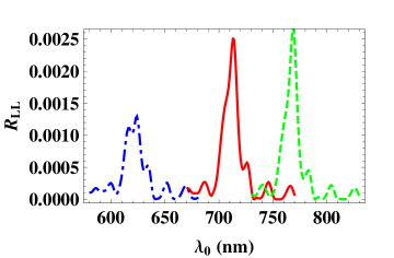
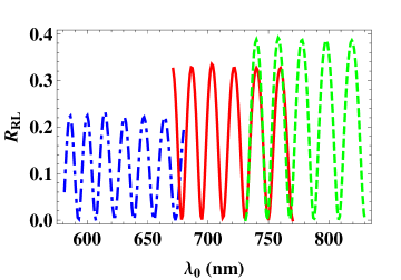
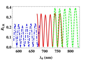
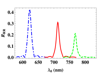
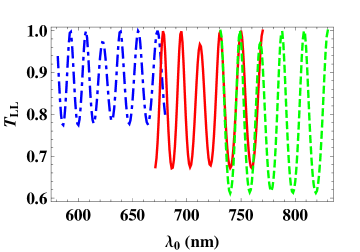
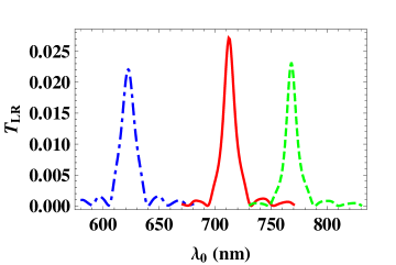
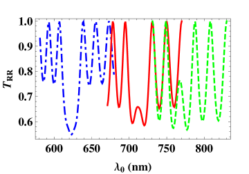
Figure 1: Reflectances and transmittances plotted against the free-space wavelength for a defect-free titanium-oxide CSTF; $L=40\Omega$, $\Omega=185$ nm, $h=+1$, $\chi_{v}=15^{\circ}$, and $\theta=10^{\circ}$. The CSTF is infiltrated with a fluid of refractive index $n_{\ell}=1.0$ (blue broken-dashed curves), $1.3$ (red solid curves), and 1.5 (green dashed curves).

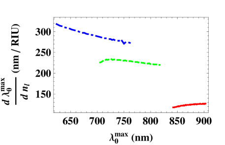
Figure 2: Spectral-shift sensitivity $d\lambda^{max}_{0}/dn_{\ell}$ plotted against $\lambda^{max}_{0}$ for $n_{\ell}\in\left(1,1.5\right)$. The vapor flux angle $\chi_{v}=15^{\circ}$ (blue broken-dashed curve), $30^{\circ}$ (green dashed curve), and $60^{\circ}$ (red solid curve).

Figure 3: Spectral-shift sensitivity as estimated by $d\lambda^{Br}_{0}/dn_{\ell}$ plotted against $\lambda^{Br}_{0}$ for $n_{\ell}\in\left(1,1.5\right)$. The vapor flux angle $\chi_{v}=15^{\circ}$ (blue broken-dashed curve), $30^{\circ}$ (green dashed curve), and $60^{\circ}$ (red solid curve).

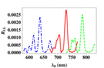
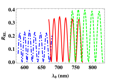
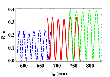
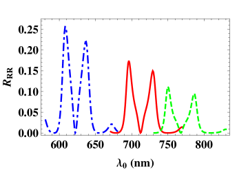
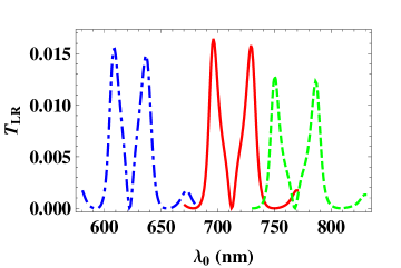
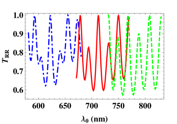
Figure 4: As Fig. 1 except that the upper half $z\in\left[L/2,L\right]$ of the CSTF is twisted about the $z$ axis by $\pi/2$ radians with respect to the lower half $z\in\left[0,L/2\right)$.

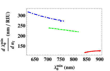
Figure 5: Spectral-shift sensitivity $d\lambda^{min}_{0}/dn_{\ell}$ plotted against $\lambda^{min}_{0}$ for $n_{\ell}\in\left(1,1.5\right)$. The vapor flux angle $\chi_{v}=15^{\circ}$ (blue broken-dashed curve), $30^{\circ}$ (green dashed curve), and $60^{\circ}$ (red solid curve).

References

• [1] A. Lakhtakia, R. Messier, M. J. Brett, and K. Robbie, โ€œSculptured thin films (STFs) for optical, chemical and biological applications,โ€ Innovations Mater. Res., vol. 1, pp.ย 165-176, 1996.
• [2] I. Hodgkinson and Q. h. Wu, โ€œInorganic chiral optical materials,โ€ Adv. Mater., vol. 13, pp. 889-897, 2001.
• [3] A. Lakhtakia and R. Messier, Sculptured Thin Films: Nanoengineered Morphology and Optics, SPIE Press, Bellingham, WA, USA, 2005.
• [4] P. G. de Gennes and J. Prost, The Physics of Liquid Crystals, Oxford University Press, New York, NY, USA, 1993.
• [5] Q. Wu, I. J. Hodgkinson, and A. Lakhtakia, โ€œCircular polarization filters made of chiral sculptured thin films: experimental and simulation results,โ€ Opt. Eng., vol. 39, pp. 1863-1868, 2000.
• [6] I. J. Hodgkinson, Q. H. Wu, A. Lakhtakia, and M. W. McCall, โ€œSpectral-hole filter fabricated using sculptured thin-film technology,โ€ Opt. Commun., vol. 177, pp. 79-84, 2000.
• [7] E. Ertekin and A. Lakhtakia, โ€œSculptured thin film Sฬ†olc filters for optical sensing of gas concentration,โ€ Eur. Phys. J. Appl. Phys., vol. 5, pp. 45-50, 1999.
• [8] J. A. Polo Jr., โ€œSculptured thin films,โ€ in Micromanufacturing and Nanotechnology, N.ย P. Mahalik, Ed., Springer, Heidelberg, Germany, 2005, pp. 357-381.
• [9] A. Lakhtakia, M. C. Demirel, M. W. Horn, and J. Xu, โ€œSix emerging directions in sculptured-thin-film research,โ€ Adv. Solid State Phys., vol. 46, pp. 295-307, 2007.
• [10] R. Messier, V. C. Venugopal, and P. D. Sunal, โ€œOrigin and evolution of sculptured thin films,โ€ J. Vac. Sci. Technol. A, vol. 18, pp. 1538-1545, 2000.
• [11] J. Xu, A. Lakhtakia, J. Liou, A. Chen, and I. J. Hodgkinson, โ€œCircularly polarized fluorescence from light-emitting microcavities with sculptured-thin-film chiral reflectors,โ€ Opt. Commun., vol. 264, pp. 235-239, 2006.
• [12] F. Zhang, J. Xu, A. Lakhtakia, S. M. Pursel, and M. W. Horn, โ€œCircularly polarized emission from colloidal nanocrystal quantum dots confined in microcavities formed by chiral mirrors,โ€ Appl. Phys. Lett., vol. 91, 023102, 2007. [Interchange the labels LCP and RCP in Fig. 2c of this paper.]
• [13] A. Lakhtakia, โ€œOn bioluminescent emission from chiral sculptured thin films,โ€ Opt. Commun., vol. 188, pp. 313-320, 2001.
• [14] T. G. Mackay and A. Lakhtakia, โ€œTheory of light emission from a dipole source embedded in a chiral sculptured thin film,โ€ Opt. Express, vol. 15, pp. 14689-14703, 2007. Erratum: vol. 16, p. 3659, 2008.
• [15] Y.-C. Yang, C.-S. Kee, J.-E. Kim, and H. Y. Park, โ€œPhotonic defect modes of cholesteric liquid crystals,โ€ Phys. Rev. E vol. 60, pp. 6852 6854, 1999.
• [16] A. Lakhtakia and M. McCall, โ€œSculptured thin films as ultranarrow-bandpass circular-polarization filters,โ€ Opt. Commun., vol. 168, pp. 457-465, 1999.
• [17] I. J. Hodgkinson, Q. H. Wu, K. E. Thorn, A. Lakhtakia, and M. W. McCall, โ€œSpacerless circular-polarization spectral-hole filters using chiral sculptured thin films: theory and experiment,โ€ Opt. Commun., vol. 184, pp. 57-66, 2000.
• [18] A. Lakhtakia, M. W. McCall, J. A. Sherwin, Q. H. Wu, and I. J. Hodgkinson, โ€œSculptured-thin-film spectral holes for optical sensing of fluids,โ€ Opt. Commun., vol. 194, pp. 33-46, 2001.
• [19] S. M. Pursel and M. W. Horn, โ€œProspects for nanowire sculptured-thin-film devices,โ€ J. Vac. Sci. Technol. B, vol. 25, pp. 2611-2615, 2007.
• [20] T. G. Mackay and A. Lakhtakia, โ€œDetermination of constitutive and morphological parameters of columnar thin films by inverse homogenization,โ€ ๐—๐—๐—๐—‰://๐–บ๐—‹๐—‘๐—‚๐—.๐—ˆ๐—‹๐—€/๐–บ๐–ป๐—Œ/0909.5375\mathsf{http://arxiv.org/abs/0909.5375}
• [21] I. Hodgkinson, Q. h. Wu, and J. Hazel, โ€œEmpirical equations for the principal refractive indices and column angle of obliquely deposited films of tantalum oxide, titanium oxide, and zirconium oxide,โ€ Appl. Opt., vol. 37, pp. 2653-2659, 1998.
• [22] R. Messier, T. Takamori, and R. Roy, โ€œStructure-composition variation in rf-sputtered films of Ge caused by process parameter changes,โ€ J. Vac. Sci. Technol., vol. 13, pp. 1060-1065, 1976.
• [23] J. R. Blanco, P. J. McMarr, J. E. Yehoda, K. Vedam, and R. Messier, โ€œDensity of amorphous germanium films by spectroscopic ellipsometry,โ€ J. Vac. Sci. Technol. A, vol. 4, pp. 577-582, 1986.
• [24] F. Walbel, E. Ritter, and R. Linsbod, โ€œProperties of TiO${}_{\mbox{x}}$ films prepared by electron-beam evaporation of titanium and titanium suboxides,โ€ Appl. Opt., vol. 42, pp. 4590-4593, 2003.
• [25] J.ย A. Sherwin, A. Lakhtakia, and I.ย J. Hodgkinson, โ€œOn calibration of a nominal structure-property relationship model for chiral sculptured thin films by axial transmittance measurements,โ€ Opt. Commun., vol. 209, pp. 369-375, 2002.
• [26] A. Lakhtakia, โ€œEnhancement of optical activity of chiral sculptured thin films by suitable infiltration of void regions,โ€ Optik, vol. 112, pp. 145-148, 2001. Erratum: vol. 112, p. 544, 2001.
• [27] T. G. Mackay and A. Lakhtakia, Electromagnetic Anisotropy and Bianisotropy: A Field Guide, Word Scientific, Singapore, 2010.
• [28] A. Lakhtakia, V. C. Venugopal, and M. W. McCall, โ€œSpectral holes in Bragg reflection from chiral sculptured thin films: circular polarization filter,โ€ Opt. Commun., vol. 177, pp. 57-68, 2000.
• [29] V. C. Venugopal and A. Lakhtakia, โ€œOn absorption by non-axially excited slabs of dielectric thin-film helicoidal bianisotropic mediums,โ€ Eur. Phys. J. Appl. Phys., vol. 10, pp. 173-184, 2000.
$\chi_{v}$ $\gamma_{b}$ $f$ nssubscript๐‘›๐‘ n_{s}