Different orderings in the narrow-band limit of the extended Hubbard model on the Bethe lattice

Abstract

We present the exact solution of a system of Fermi particles living on the sites of a Bethe lattice with coordination number $z$ and interacting through on-site $U$ and nearest-neighbor $V$ interactions. This is a physical realization of the extended Hubbard model in the atomic limit. Within the Green’s function and equations of motion formalism, we provide a comprehensive analysis of the model and we study the phase diagram at finite temperature in the whole model’s parameter space, allowing for the on-site and nearest-neighbor interactions to be either repulsive or attractive. We find the existence of critical regions where charge ordering ($V>0$) and phase separation ($V<0$) are observed. This scenario is endorsed by the study of several thermodynamic quantities.

I Introduction

In recent years, many theoretical as well as experimental investigations in condensed matter physics have been devoted to the study of low-dimensional strongly correlated electron systems where long-range Coulomb interactions play an important role. A crucial problem is to understand the effects of competing interactions and the corresponding phase transitions. One of the seminal models adopted to take into account long-range Coulomb interactions is the so-called extended Hubbard model (EHM), which, beside the on-site interaction $U$, contains also a nearest-neighbor interaction $V$. Although the EHM looks deceptively simple and in spite of a very intensive study, both analytical and numerical, there is no complete exact solution even in $1D$. These difficulties have led to the investigation of the so-called atomic limit of the extended Hubbard model (AL-EHM). According to the conventional definition used in the literature, the atomic limit stands for the classical limit of the model, where the hopping matrix elements $t_{ij}$ are set to zero from the very beginning. The AL-EHM is exactly solvable in one dimension (see Ref. mancini08_PRE and references therein), as well as when it is defined on the Bethe lattice mancini08_1 ; mancini08_2 . Here we consider the Bethe lattice as the infinite version of a Cayley tree; thus we are not concerned with surface effects. The Bethe lattice, beside being an useful framework for studying the electronic structure of amorphous and glassy solids, has a relevant role in condensed matter physics and statistical mechanics. Due to its peculiar structure, on the Bethe lattice it is possible to exactly solve several interesting physical problems involving interactions baxter . There are two special properties that make Bethe lattices particularly suited for theoretical investigations: the self-similar structure which may lead to recursive solutions and the absence of closed loops which restricts interference effects of quantum-mechanical particles in the case of nearest-neighbor coupling. Furthermore, Bethe and Bethe-like lattices have attracted a lot of interest because they usually reflect essential features of systems even when conventional mean-field theories fail bethe . The reason is that such lattices are capable to take into account correlations which are usually lost in conventional mean-field calculations. Very recently, the Bethe lattice has been considered as the underlying lattice to study the suppression of the paramagnetic metal-insulator transition in the Hubbard model at half-filling in the presence of nearest-neighbor and next-nearest-neighbor hoppings when the latter is increased with respect to the former NNN1 ; NNN2 . Furthermore, there exist in nature hyperbranched polymers with distinct regular molecular architecture (so-called dendrimers) which can be conveniently modelized by a Bethe-like Hamiltonian dendrimers1 ; dendrimers2 ; dendrimers3 .

In this article, we study the AL-EHM on the Bethe lattice by means of the equations of motion approach mancini_avella_04 . For one-dimensional lattices, or more generally for lattices with no closed loops, classical fermionic and spin systems can be easily solved by means of the transfer matrix method baxter . However, this method is hardy implementable when more complex lattices are considered. The Onsager solution for the two-dimensional Ising model is an emblematic example onsager . We feel that there is the necessity to foster alternative methods which can be used for a large class of lattices. In Ref. mancini_05 we have shown that the equations of motion method provides an answer to this exigency. By using this method, localized fermionic systems and Ising-like models can be in principle solved for any underlying lattice. Indeed, one can find a set of eigenenergies and eigenoperators of the Hamiltonian which closes the hierarchy of the equations of motion. As a result, one can derive exact analytical expressions for the relevant Green’s functions and correlation functions, which turn out to depend on a finite set of parameters. The knowledge of these parameters is essential to obtain a solution of these models. In a series of articles mancini08_PRE ; mancini08_1 ; mancini08_2 ; mancini_05 ; mancini_05_2 ; mancini_naddeo_06 ; spin32 ; cmp , we have analyzed several fermionic and spin systems and we have developed a self-consistent method which allows us to determine these parameters for the case of one-dimensional and Bethe lattices. Some preliminary results for the AL-EHM on the Bethe lattice were presented in Refs. mancini08_1 ; mancini08_2 , where we considered only the case of attractive intersite interactions ($V<0$). Upon varying the temperature, we found a region of negative compressibility, hinting at a transition from a thermodynamically stable to an unstable phase, characterized by phase separation. In this paper, we provide a comprehensive and systematic exact analysis of the AL-EHM on the Bethe lattice with coordination number $z$ by considering relevant response and correlation functions as well as thermodynamic quantities. We consider both the cases $V<0$ and $V>0$ and cover a wide range of values of the parameters $n$, $T$ and $U$ ($n$ is the particle density and $T$ the temperature). The possibility for the parameters $U$ and $V$ to take positive as well as negative values - representing effective interaction couplings taking into account also other interactions (for instance with phonons) - gives rise to a rich phenomenology and a variety of phases. In particular, the ratio of the two competing terms in the model Hamiltonian, i.e., the on-site and the intersite interactions, determines the different distributions of the electrons and the accessible phases, which we identified as charge ordered (CO) or phase separated (PS). Indeed, several studies of the EHM on regular lattices have pointed at the presence of states with phase separation pha_sep ; dongen_95 ; lin_00 ; tong_04 and of charge-ordered phases lin_00 ; tong_04 ; pietig_99 ; hoang_02 ; seo_06 ; pawl_06 . Furthermore, the introduction of an intersite interaction can mimic longer-ranged Coulomb interactions needed to describe effects observed in conducting polymers baeriswyl_92 . In this article, we report the phase diagram in the space ($U,n,T$) showing the existence of critical regions where charge ordering ($V>0$) and phase separation ($V<0$) are observed. These studies have not been reported in the literature and bring some more information on the properties of the Hubbard model.

The plan of the paper is as follows. In Sec. II, we review and extend the analysis of the AL-EHM defined on a Bethe lattice with coordination number $z$ leading to the computation of the Green’s and correlation functions mancini08_1 ; mancini08_2 . In Sec. III, the attractive $V$ case is reviewed in detail and the phase diagram is reported for a wide range of values of the external parameters $n$, $T/\left|V\right|$, $U/\left|V\right|$. In Sec. IV, we investigate the case of repulsive intersite interactions. The phase diagram in the space $n$, $T/V$, $U/V$ is derived and a long-range CO state is observed. The lattice is characterized by a inhomogeneous distribution of the particles in alternating shells. Relevant thermodynamic quantities - such as the specific heat, susceptibility, entropy - are also investigated as functions of the temperature, on-site potential and particle density. Finally, Sec. V is devoted to our concluding remarks while the appendix reports some relevant computational details.

II The Hamiltonian and the equations of motion

The theoretical framework leading to the exact solution of the AL-EHM defined on the Bethe lattice has been already reported in Refs. mancini08_1 ; mancini08_2 . In this Section we shall review the analysis and extend it, considering also the breaking of translational invariance and the addition of an external magnetic field.

In the extended Hubbard model, a nearest-neighbor interaction $V$ is added to the original Hubbard Hamiltonian, which contains only an on-site interaction $U$:

$$\begin{split}H&=\sum_{\langle\bf ij\rangle}[t_{\bf ij}-\delta_{\bf ij}\,\mu]c^{\dagger}(i)c(j)+U\sum_{i}{n_{\uparrow}(i)n_{\downarrow}(i)}\\ &+\frac{1}{2}\sum_{\langle\bf ij\rangle}V_{\bf ij}\,n(i)n(j).\end{split}$$ (1)

$U$ and $V$ are the strengths of the local and intersite interactions, respectively; $\mu$ is the chemical potential, $n(i)=n_{\uparrow}(i)+n_{\downarrow}(i)$ and $D(i)=n_{\uparrow}(i)n_{\downarrow}(i)=n\left(i\right)\left[n\left(i\right)-1\right]/2$ are the particle density and double occupancy operators, respectively, at site $\bf i$; $t_{\bf ij}$ is the hopping matrix. As usual, $n_{\sigma}(i)=c_{\sigma}^{{\dagger}}(i)c_{\sigma}(i)$ with $\sigma=\left\{{\uparrow,\downarrow}\right\}$ where $c_{\sigma}(i)$ ($c_{\sigma}^{{\dagger}}(i))$ is the fermionic annihilation (creation) operator of an electron of spin $\sigma$ at site $\bf{i}$, satisfying canonical anticommutation relations. We use the Heisenberg picture: $i=\left({\bf i},t\right)$, where $\bf{i}$ stands for the lattice vector $\bf{R}_{i}$. In the extreme narrow-band (atomic) limit the Hamiltonian (1) becomes

$$H=-\mu\sum_{\bf i}n(i)+U\sum_{\bf i}D(i)+\frac{1}{2}\sum_{\langle\bf ij\rangle}V_{\bf ij}\,n(i)n(j).$$ (2)

We shall study this model on a Bethe lattice with coordination number $z$. For this lattice, the Hamiltonian (2) can be conveniently rewritten as

$$H=-\mu n(0)+UD(0)+\sum_{p=1}^{z}H^{(p)}.$$ (3)

$H^{(p)}$ is the Hamiltonian of the $p$-th sub-tree rooted at the central site $(0)$ and can be written as

$$H^{(p)}=-\mu\,n(p)+UD(p)+Vn(0)n(p)+\sum_{m=1}^{z-1}H^{(p,m)}.$$ (4)

Here $(p)$ ($p=1,\ldots z)$ are the nearest-neighbor sites of $(0)$, also termed the first shell. $H^{(p,m)}$ describes the $m$-th sub-tree rooted at the site ($p$); $(p,m)$ ($m=1,\ldots z-1)$ and $(0)$ are the nearest-neighbors of the site ($p$). The process may be continued indefinitely.

The equations of motion approach in the context of the composite operator method mancini_avella_04 - based on the choice of a convenient operatorial basis - provides us with the exact solution of the model. For our purposes, the suitable field operators are the Hubbard operators, $\xi(i)=[1-n(i)]c(i)$ and $\eta(i)=n(i)c(i)$, which satisfy the equations of motion:

$$\begin{split}i\frac{\partial}{\partial t}\xi(i)&=-\mu\xi(i)+zV\xi(i)n^{\alpha}(i),\\ i\frac{\partial}{\partial t}\eta(i)&=(U-\mu)\eta(i)+zV\eta(i)n^{\alpha}(i).\end{split}$$ (5)

In the following, for a generic operator $\Phi\left(i\right)$ we shall use the notation $\Phi^{\alpha}(i)=\sum\nolimits_{p=1}^{z}\Phi(i,p)/z$, where $(i,p)$ are the first nearest-neighbors of the site $i$. The Heisenberg equations (5) contain the higher-order nonlocal operators $\xi(i)n^{\alpha}(i)$ and $\eta(i)n^{\alpha}(i)$. By taking time derivatives of the latter, higher-order operators are generated. This process may be continued and an infinite hierarchy of field operators is created. However, since the number $n(i)$ and the double occupancy $D(i)$ operators satisfy the following algebra

$$\begin{split}n^{p}\left(i\right)&=n\left(i\right)+a_{p}D(i),\\ D^{p}\left(i\right)&=D(i),\\ n^{p}\left(i\right)D(i)&=2D(i)+a_{p}D(i),\end{split}$$ (6)

where $p\geq 1$ and $a_{p}=2^{p}-2$, it is straightforward to establish the following recursion rule mancini_05 ; mancini_05_2 :

$$[n^{\alpha}(i)]^{k}=\sum_{m=1}^{2z}A_{m}^{(k)}[n^{\alpha}(i)]^{m}.$$ (7)

The coefficients $A_{m}^{(k)}$ are rational numbers, satisfying the relations $\sum_{m=1}^{2z}A_{m}^{(k)}=1$ and $A_{m}^{(k)}=\delta_{m,k}$ $(k=1,\ldots,2z)$ mancini08_PRE ; mancini_epjb_05 . The recursion relation (7) allows one to close the hierarchy of equations of motion.

II.1 Eigenoperators and eigenvalues

One may define the composite field operator

$$\psi(i)=\left(\begin{array}[]{*{20}c}{\psi^{(\xi)}(i)}\\ {\psi^{(\eta)}(i)}\\ \end{array}\right),$$ (8)

where

$$\psi^{(\xi)}(i)=\left({{\begin{array}[]{*{20}c}{\xi(i)}\\ {\xi(i)[n^{\alpha}(i)]}\\ \vdots\\ {\xi(i)[n^{\alpha}(i)]^{2z}}\\ \end{array}}}\right),\;\psi^{(\eta)}(i)=\left({{\begin{array}[]{*{20}c}{\eta(i)}\\ {\eta(i)[n^{\alpha}(i)]}\\ \vdots\\ {\eta(i)[n^{\alpha}(i)]^{2z}}\\ \end{array}}}\right).$$ (9)

By using the recursion rule (7), one can show that the fields $\psi^{(\xi)}(i)$ and $\psi^{(\eta)}(i)$ are eigenoperators of the Hamiltonian (3) mancini08_1 ; mancini08_2 :

$$\begin{split}i\frac{\partial}{\partial t}\psi^{(\xi)}(i)&=[\psi^{(\xi)}(i),H]=\varepsilon^{(\xi)}\psi^{(\xi)}(i),\\ i\frac{\partial}{\partial t}\psi^{(\eta)}(i)&=[\psi^{(\eta)}(i),H]=\varepsilon^{(\eta)}\psi^{(\eta)}(i),\end{split}$$ (10)

where $\varepsilon^{(\xi)}$ and $\varepsilon^{(\eta)}$ are the $(2z+1)\times(2z+1)$ energy matrices

$$\varepsilon^{(\xi)}=\left({{\begin{array}[]{*{20}c}{-\mu}&{zV}&0\hfill&\cdots&0&0&0\\ 0&{-\mu}&{zV}&\cdots&0&0&0\\ 0&0&{-\mu}&\cdots&0&0&0\\ \vdots&\vdots&\vdots&\cdots&\vdots&\vdots&\vdots\\ 0&0&0&\cdots&{-\mu}&{zV}&0\\ 0&0&0&\cdots&0&{-\mu}&{zV}\\ 0&{zVA_{1}^{(2z+1)}}&{zVA_{2}^{(2z+1)}}&\cdots&{zVA_{2z-2}^{(2z+1)}}&{zVA_{2z-1}^{(2z+1)}}&{-\mu+zVA_{2z}^{(2z+1)}}\\ \end{array}}}\right)$$ (11)

$$\varepsilon^{(\eta)}=\left({{\begin{array}[]{*{20}c}{U-\mu}&{zV}&0&\cdots&0&0&0\\ 0&{U-\mu}&{zV}&\cdots&0&0&0\\ 0&0&{U-\mu}&\cdots&0&0&0\\ \vdots&\vdots&\vdots&\cdots&\vdots&\vdots&\vdots\\ 0&0&0&\cdots&{U-\mu}&{zV}&0\\ 0&0&0&\cdots&0&{U-\mu}&{zV}\\ 0&{zVA_{1}^{(2z+1)}}&{zVA_{2}^{(2z+1)}}&\cdots&{zVA_{2z-2}^{(2z+1)}}&{zVA_{2z-1}^{(2z+1)}}&{U-\mu+zVA_{2z}^{(2z+1)}}\\ \end{array}}}\right)$$ (12)

whose eigenvalues, $E_{m}^{(\xi)}$ and $E_{m}^{(\eta)}$, are given by:

$$\begin{split}E_{m}^{(\xi)}&=-\mu+(m-1)V,\\ E_{m}^{(\eta)}&=-\mu+U+(m-1)V,\end{split}$$ (13)

with $m=1,\ldots,2z+1$. The Hamiltonian has now been formally solved since, for any coordination number of the underlying Bethe lattice, one has found a closed set of eigenoperators and eigenenergies. As a result, one may compute observable quantities. This will be done in the next section by using the formalism of Green’s functions (GF).

II.2 Retarded Green’s functions and correlation functions

The knowledge of a set of eigenoperators and eigenenergies of the Hamiltonian allows one to find an exact expression for the retarded Green’s function

$$G^{(s)}(t-t^{\prime})=\theta(t-t^{\prime})\langle\{\psi^{(s)}({\bf i},t),{\psi^{(s)}}^{\dagger}({\bf i},t^{\prime})\}\rangle,$$ (14)

and, consequently, for the correlation function

$$C^{(s)}(t-t^{\prime})=\langle\psi^{(s)}({\bf i},t){\psi^{(s)}}^{\dagger}({\bf i},t^{\prime})\rangle.$$ (15)

In the above equations, $s=\xi,\eta$ and $\langle\cdots\rangle$ denotes the quantum-statistical average over the grand canonical ensemble. It is not difficult to show that, for fermionic operators, only the on-site correlations are non-zero. It is not difficult to show that the retarded GF and satisfies the equation

$$\left[{\omega-\varepsilon^{(s)}}\right]G^{(s)}(\omega)=I^{(s)},$$ (16)

where $G^{(s)}(\omega)$ is the Fourier transform of $G^{\left(s\right)}(t-{t}^{\prime})$ and $I^{(s)}=\langle\{\psi^{(s)}(i),{\psi^{(s)}}^{\dagger}(i)\}\rangle$ is the $(2z+1)\times(2z+1)$ normalization matrix. The solution of Eq. (16) is mancini_avella_04 :

$$G^{(s)}(\omega)=\sum_{m=1}^{2z+1}\frac{\sigma^{(s,m)}}{\omega-E_{m}^{(s)}+i\delta}.$$ (17)

Similarly, the correlation function satisfies the equation

$$C^{(s)}(\omega)=-\left[{1+\tanh\frac{\beta\omega}{2}}\right]\,{\rm Im}\left[{G^{(s)}(\omega)}\right],$$ (18)

where $C^{(s)}(\omega)$ is the Fourier transform of $C^{(s)}(t-{t}^{\prime})$, whose solution is

$$C^{(s)}(\omega)=\pi\sum_{m=1}^{2z+1}\sigma^{(s,m)}\,T_{m}^{(s)}\,\delta(\omega-E_{m}^{(s)}).$$ (19)

In the above equations, $T_{m}^{(s)}=1+\tanh\big{(}\beta E_{m}^{(s)}/2\big{)}$, $\beta=1/k_{B}T$ and the $E_{m}^{(s)}$ are given in Eq. (13). The spectral density matrices $\sigma_{ab}^{(s,n)}$ can be computed by means of the formula mancini_avella_04 :

$$\sigma_{ab}^{(s,n)}=\Omega_{an}^{(s)}\sum_{c=1}^{2z+1}\left[{\Omega_{nc}^{(s)}}\right]^{-1}I_{cb}^{(s)}.$$ (20)

In Eq. (20), $\Omega^{(s)}$ is the $(2z+1)\times(2z+1)$ matrix whose columns are the eigenvectors of the energy matrix $\varepsilon^{(s)}$. $I_{a,b}^{(s)}$ are instead the elements of the normalization matrix $I^{(s)}$. Calculations show that $\Omega^{(\xi)}=\Omega^{(\eta)}=\Omega$, with the matrix $\Omega$ given by

$$\Omega_{p,k}=\left\{{{\begin{array}[]{*{20}c}1\\ 0\\ {\left({\frac{z}{k-1}}\right)^{2z+1-p}}\\ \end{array}}}\right.\quad\quad{\begin{array}[]{*{20}c}{k=1,\;p=1},\\ {k=1,\;p\neq 1},\\ {k\neq 1}.\\ \end{array}}$$ (21)

The matrix elements of the normalization matrices $I^{(s)}$ have the expressions

$$I_{n,m}^{(\xi)}=\kappa^{(n+m-2)}-\lambda^{(n+m-2)},\quad I_{n,m}^{(\eta)}=\lambda^{(n+m-2)},$$ (22)

where the correlators $\kappa^{(p)}$ and $\lambda^{(p)}$ are defined as

$$\kappa^{(p)}=\langle[n^{\alpha}(i)]^{p}\rangle,\quad\lambda^{(p)}=\frac{1}{2}\langle n(i)[n^{\alpha}(i)]^{p}\rangle.$$ (23)

By exploiting the recursion relation (7), it is not difficult to show that also $\kappa^{(p)}$ and $\lambda^{(p)}$ obey similar recursion relations

$$\kappa^{(p)}=\sum_{m=1}^{2z}A_{m}^{(p)}\kappa^{(m)},\quad\lambda^{(p)}=\sum_{m=1}^{2z}A_{m}^{(p)}\lambda^{(m)},$$ (24)

limiting their computation to the first $2z$ correlators mancini08_1 . At this stage, the knowledge of the GFs and of the CFs is not yet achieved since they depend on the $\{\sigma^{(s,m)}\}$ which, in turn, depend on the normalization matrix elements: there are $2z$ parameters to determine. To find these parameters, we shall exploit the Pauli principle and impose pertinent boundary conditions for obtaining a set of self-consistent equations.

One first chooses an arbitrary site, say ${\bf i}$, then splits the Hamiltonian (3) in the sum of two terms: $H=H_{0}^{(i)}+H_{I}^{(i)}$, where

$$\begin{split}H_{0}^{(i)}&=-\mu[n(i)+zn^{\alpha}(i)]+U[D(i)+zD^{\alpha}(i)]\\ &+\sum_{p=1}^{z}\sum_{m=1}^{z-1}H^{(p,m)},\\ H_{I}^{(i)}&=zVn(i)n^{\alpha}(i),\end{split}$$ (25)

and introduce the $H_{0}^{(i)}$-representation: the statistical average of any operator $O$ can be expressed as

$$\langle O\rangle=\frac{\langle Oe^{-\beta H_{I}^{(i)}}\rangle_{0,\bf i}}{\langle e^{-\beta H_{I}^{(i)}}\rangle_{0,\bf i}}.$$ (26)

The symbol $\langle\cdots\rangle_{0,\bf i}$ stands for the thermal average with respect to the reduced Hamiltonian $H_{0}^{(i)}$: i.e., $\langle\cdots\rangle_{0,\bf i}=Tr\{\cdots e^{-\beta H_{0}^{(i)}}\}/Tr\{e^{-\beta H_{0}^{(i)}}\}$. Equation (26) allows us to express the thermal averages with respect to the complete Hamiltonian $H$ in terms of thermal averages with respect to the reduced Hamiltonian $H_{0}$, which describes a system where the original lattice has been reduced to the site ${\bf i}$ and to $z$ unconnected sublattices. As a consequence, in the $H_{0}$-representation, correlation functions connecting sites belonging to disconnected sublattices can be decoupled. Let us consider the correlation functions

$$C_{1,k}^{(s)}=\langle{s(i)s^{\dagger}(i)\left[{n^{\alpha}\left(i\right)}\right]^{k-1}}\rangle,$$ (27)

where $s=\xi,\eta$ and $k=1,...,2z+1$. By means of Eq. (26), they can be written as:

$$C_{1,k}^{(s)}=\frac{\langle s(i)s^{\dagger}(i)\left[n^{\alpha}(i)\right]^{k-1}e^{-\beta H_{I}}\rangle_{0,\bf i}}{\langle e^{-\beta H_{I}}\rangle_{0,\bf i}}.$$ (28)

The Pauli principle leads to the following algebraic relations

$$\begin{split}\xi^{\dagger}(i)n(i)&=0,\\ \xi^{\dagger}(i)D(i)&=0,\end{split}\quad\quad\quad\begin{split}\eta^{\dagger}(i)n(i)&=\eta^{\dagger}(i),\\ \eta^{\dagger}(i)D(i)&=0,\end{split}$$ (29)

from which one has $\xi^{\dagger}(i)\,e^{-\beta H_{I}}=\xi^{\dagger}(i)$, and $\eta^{\dagger}(i)\,e^{-\beta H_{I}}=\eta^{\dagger}(i)\,e^{-z\beta Vn^{\alpha}(i)}$. In the $H_{0}$-representation, the correlation functions can be rewritten as:

$$\begin{split}C_{1,k}^{(\xi)}&=\frac{\langle{\xi(i)\xi^{\dagger}(i)}\rangle_{0,\bf i}\langle{[n^{\alpha}(i)]^{k-1}}\rangle_{0,\bf i}}{\langle{e^{-\beta H_{I}}}\rangle_{0,\bf i}},\\ C_{1,k}^{(\eta)}&=\frac{\langle{\eta(i)\eta^{\dagger}(i)}\rangle_{0,\bf i}\langle{[n^{\alpha}(i)]^{k-1}e^{-z\beta Vn^{\alpha}(i)}}\rangle_{0,\bf i}}{\langle{e^{-\beta H_{I}}}\rangle_{0,\bf i}}.\end{split}$$ (30)

In the $H_{0}$-representation, the Hubbard operators obey to simple equations of motion: $[\xi(i),H_{0}]=-\mu\,\xi(i)$ and $[\eta(i),H_{0}]=-(\mu-U)\,\eta(i)$. Thus, it is easy to show that the equal time CF’s can be expressed as:

$$\begin{split}\langle{\xi(i)\xi^{\dagger}(i)}\rangle_{0,\bf i}&=\frac{1}{1+2e^{\beta\mu}+e^{\beta(2\mu-U)}}=1-B_{1}+B_{2},\\ \langle{\eta(i)\eta^{\dagger}(i)}\rangle_{0,\bf i}&=\frac{e^{\beta\mu}}{1+2e^{\beta\mu}+e^{\beta(2\mu-U)}}=\frac{1}{2}\left(B_{1}-2B_{2}\right),\end{split}$$ (31)

where:

$$\begin{split}B_{1}&=\langle n(i)\rangle_{0,\bf i}=\frac{2(f+g)}{1+2f+g},\\ B_{2}&=\langle D(i)\rangle_{0,\bf i}=\frac{g}{1+2f+g}.\end{split}$$ (32)

In Eq. (32), we have defined $f=e^{\beta\mu}$, $g=e^{\beta(2\mu-U)}$, and we have used the identities

$$\begin{split}&\xi_{\sigma}\xi_{\sigma}^{\dagger}+\eta_{\sigma}\eta_{\sigma}^{\dagger}=1-n_{\sigma},\\ &\eta_{\sigma}\eta_{\sigma}^{\dagger}=n_{\sigma}-n_{\uparrow}n_{\downarrow}.\end{split}$$ (33)

Upon inserting Eqs. (31) into Eqs. (30) and by taking $k=1$, one finds:

$$\begin{split}C_{1,1}^{(\xi)}&=\frac{1-B_{1}+B_{2}}{\langle e^{-\beta H_{I}}\rangle_{0,\bf i}},\\ C_{1,1}^{(\eta)}&=\frac{\left({B_{1}-2B_{2}}\right)\langle e^{-z\beta Vn^{\alpha}(0)}\rangle_{0,\bf i}}{2\langle e^{-\beta H_{I}}\rangle_{0,\bf i}}.\end{split}$$ (34)

It is not difficult to show that the averages in the above equations can be expressed as:

$$\begin{split}&\langle e^{-\beta H_{I}^{(i)}}\rangle_{0,\bf i}=1+B_{1}\left(F_{i}^{z}-1\right)+B_{2}\left(1-2F_{i}^{z}+G_{i}^{z}\right),\\ &\langle{e^{-z\beta Vn^{\alpha}(0)}}\rangle_{0,\bf i}=F_{i}^{z},\end{split}$$ (35)

where

$$F_{i}=1+aX_{i}+a^{2}Y_{i},\quad G_{i}=1+dX_{i}+d^{2}Y_{i}.$$ (36)

In the above equations we have defined $a=K-1$, $d=K^{2}-1$, with $K=e^{-\beta V}$; $i_{p}$ ($p=1,\ldots,z$) is an arbitrary neighboring site of $i$. $X_{i}$ and $Y_{i}$ are two parameters defined as:

$$\begin{split}X_{i}&=\langle n^{\alpha}(i)\rangle_{0,\bf i}=\frac{1}{z}\sum_{p=1}^{z}\langle n(i_{p})\rangle_{0,\bf i},\\ Y_{i}&=\langle D^{\alpha}(i)\rangle_{0,\bf i}=\frac{1}{z}\sum_{p=1}^{z}\langle D(i_{p})\rangle_{0,\bf i}.\end{split}$$ (37)

$X_{i}$ and $Y_{i}$ are parameters of seminal importance since all correlators and fundamental properties of the system under study can be expressed in terms of them. Relevant physical quantities, such as the mean value of the particle density and doubly occupancy, and the charge correlators $\kappa^{(k)}$ and $\lambda^{(k)}$ (23) can be easily computed. After lengthy but straightforward calculations, one finds:

$$\begin{split}\langle{n(i)}\rangle&=\frac{2f\,F_{i}^{z}+2g\,G_{i}^{z}}{1+2f\,F_{i}^{z}+g\,G_{i}^{z}},\\ \langle{D(i)}\rangle&=\frac{g\,G_{i}^{z}}{1+2f\,F_{i}^{z}+g\,G_{i}^{z}},\end{split}$$ (38)

and

$$\begin{split}\langle{n(i_{p})}\rangle&=\frac{1}{1+2f\,F_{i}^{z}+g\,G_{i}^{z}}\left[2f\,K\left({X_{i}+2aY_{i}}\right)F_{i}^{z-1}\right.\\ &+\left.g\,K^{2}\left({X_{i}+2d\,Y_{i}}\right)G_{i}^{z-1}+X_{i}\right],\\ \langle{D(i_{p})}\rangle&=\frac{Y_{i}\left(1+2fK^{2}F_{i}^{z-1}+g\,K^{4}G_{i}^{z-1}\right)}{1+2f\,F_{i}^{z}+g\,G_{i}^{z}}.\end{split}$$ (39)

The parameters $X_{i}$ and $Y_{i}$ will be fixed by using boundary conditions, which will be different according to the sign of the intersite potential $V$. Therefore, we shall consider separately the cases $V<0$ and $V>0$. For both cases we shall study, in the next sections, relevant thermodynamic quantities and response functions, such as the internal energy, the specific heat, the charge and spin susceptibilities and the entropy. The internal energy $E$ can be computed as the thermal average of the Hamiltonian (2) and it is given by $E=UD+zV\lambda^{(1)}$. The specific heat is then directly given by $C=dE/dT$. The charge susceptibility $\chi_{c}$ can be computed by means of thermodynamics through the formula

$$\chi_{c}=Nn^{2}+\frac{1}{\beta}\frac{\partial n}{\partial\mu}.$$ (40)

In the above equation, $N$ is the number of sites and $n=\sum_{i}\langle n(i)\rangle/N$ is the particle number per site. The spin magnetic susceptibility $\chi_{s}$ can be computed by introducing an external magnetic field $h$, taking the derivative of the magnetization $m=\langle n_{\uparrow}(i)-n_{\downarrow}(i)\rangle$ with respect to $h$ and letting $h$ going to zero:

$$\chi_{s}=\left(\frac{\partial m}{\partial h}\right)_{h=0}.$$ (41)

The addition of a homogeneous magnetic field does not dramatically modify the framework of calculation given in this section, once one has taken into account the breakdown of the spin rotational invariance. Some details of the calculations are given in the appendix.

III Attractive intersite potential

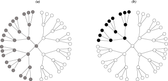
Figure 1: Distribution of the particles in the Bethe lattice at $n=0.5$ and $T=0$: ($a$) $V<0$ and $U\gtrapprox U_{PS}$; ($b$) $V<0$ and $U\lessapprox U_{PS}$. White, grey and black circles denote empty, arbitrary spin singly occupied and double occupied sites, respectively.

In this Section, we review the case of attractive intersite potential. For $V<0$, the AL-EHM on the Bethe lattice exhibits a phase separation at low temperatures mancini08_2 . This phenomenon is characterized by a macroscopically inhomogeneous ground state where different spatial regions have different average particle densities. As it has been evidenced in Ref. mancini08_2 , there exists a critical temperature $T_{c}$ below which the system loses translational invariance and phase separation occurs. Moreover, for $T<T_{c}$ two types of phase separated configurations are possible according to the strength of the on-site potential $U$: clusters of singly occupied sites or clusters of doubly occupied sites. This is qualitatively illustrated in Fig. 1, where we report just one possible configuration for $n=0.5$ and $T=0$. There is a critical value of the on-site potential $U_{PS}$, depending on the coordination number $z$ and on filling $n$, separating the two types of phase separated configurations. In the high temperature regime, one may safely assume that the system is in the translational invariant phase. Thus, one requires: $\langle n(i)\rangle=\langle n^{\alpha}(i)\rangle$ and $\langle D(i)\rangle=\langle D^{\alpha}(i)\rangle$, $\forall i$. As a consequence, from Eqs. (38) and (39), we obtain two equations allowing us to determine $X_{i}$ and $Y_{i}$ as functions of the chemical potential $\mu$:

$$X=2f(1-X-dY)F^{z-1}+g[2+(d-1)X-2dY]G^{z-1},$$ (42a)

$$Y=g[1+dX-(2d+1)Y]G^{z-1}-2fK^{2}YF^{z-1}.$$ (42b)

In the above equations, we dropped the index $i$ because all the sites are equivalent. Since experimentally, by varying the doping, it is possible to tune the density in a controlled way, here we shall fix the particle density $n=\langle n(i)\rangle$; the chemical potential will be determined by the system itself, according to the values of the external parameters, by means of the following equation:

$$n=\frac{\left(X-2Y\right)F+2YG}{1-X+Y+\left(X-2Y\right)F+YG}.$$ (43)

Equations (42b) and (43) constitute a system of coupled equations allowing one to ascertain the three parameters $\mu$, $X$ and $Y$ in terms of the external parameters of the model $n$, $U$, $V$, $T$, and $z$. Once these quantities are known, all the properties of the model can be computed. As an example, the double occupancy $D=\langle D(i)\rangle$ and the nearest-neighbor charge correlation function $\lambda^{(1)}=\langle{n(i)n^{\alpha}(i)]}\rangle$/2, in terms of $X$ and $Y$, are given by:

$$\begin{split}D&=\frac{YG}{1-X+Y+\left(X-2Y\right)F+YG},\\ \lambda^{(1)}&=\frac{K\left(X+2aY\right)\left(X-2Y\right)+2K^{2}Y\left(X+2dY\right)}{2\left(1-X+Y\right)+2\left(X-2Y\right)F+2YG}.\end{split}$$ (44)

III.1 The solution at half filling

As it has been evidenced in Ref. mancini08_1 , of particular interest is the case of half filling due to the possibility to analytically reveal the spontaneous breakdown of the particle-hole symmetry. Because of this invariance property of the Hamiltonian (3), at $n=1$ the chemical potential does not depend on the temperature and takes the constant value $\mu=U/2+zV$. Upon substituting this value of $\mu$ in Eqs. (42b), one finds that these equations admit the following solution

$$X=1-dY,$$ (45a)

with $$Y$$ determined by the equation

$$Y\left(1+K^{2}\right)+2e^{\beta U/2}KY\left(1-a^{2}Y\right)^{z-1}-1=0.$$ (45b)

It can be shown that this solution gives

$$\begin{split}n&=1,\\ D&=\frac{1}{2+2e^{\beta U/2}(1-a^{2}Y)^{z}},\\ \lambda^{(1)}&=\frac{1}{2}+dYD.\end{split}$$ (46)

That is, solution (45) satisfies the particle-hole symmetry. On the other hand, if one perturbs the solution (45a), by setting for example $X=1-dY+\delta$, it is straightforward to show that a particle-hole symmetry breaking solution exists for temperatures lower than a critical temperature $T_{c}$, determined by:

$$\begin{split}&2K^{\frac{U/\left|V\right|+2}{2}}[z+K(z-2)]^{z-1}\\ &+(K+1)^{z-1}(z-1)^{z-1}[z-K^{2}(z-2)]=0.\end{split}$$ (47)

Figure 2: The transition temperature $T_{c}$ as a function of the on-site potential $U$ for $V=-1$, $n=1$ and different values of the coordination number $z$.

Numerical calculations show that Eq. (47) admits a solution only for attractive intersite interactions. It is interesting to consider Eq. (47) in two extremal limits, namely $U/\left|V\right|\to-\infty$ and $T_{c}\to 0$. In the former limit, corresponding to the case of vanishing intersite potential, one finds the same critical temperature exhibited by a system of spinless fermions living on the sites of a Bethe lattice mancini08_1 :

$$\frac{k_{B}T_{c}}{\left|V\right|}=2\left[\ln\left({\frac{z}{z-2}}\right)\right]^{-1}$$ (48)

Since the spinless fermion model can be mapped into the spin-1/2 Ising model, our result for the critical temperature agrees with the one previously found in the literature baxter ; mancini_naddeo_06 . In the second limit, Eq. (47) becomes

$$\left({U/2-\left|V\right|}\right)=k_{B}T_{c}\ln\left[{\frac{(z-1)^{z-1}}{2(z-2)^{z-2}}}\right].$$ (49)

That is, $U=2|V|$ is the critical value of the on-site potential at which a quantum phase transition occurs. The results obtained from Eq. (47) are displayed in Fig. 2. One observes that, at fixed coordination number, by increasing $U$ from large negative values, the critical temperature decreases, and the lower the coordination number, the lower the critical temperature. An interesting feature of the phase diagram is that for $U>2|V|$, the critical temperature exhibits a reentrant behavior. The width of the reentrance increases with $z$, and the turning point is at a critical value $U_{c}$, which depends linearly on the coordination number via the law: $U_{c}/|V|=a+bz$ (for $z\geq 3$), where $a\approx 0.69$ and $b\approx 0.54$. For $z=3$ one has $U_{c}\approx 2.3|V|$.

III.2 Phase diagram and local properties

In this Subsection, we review the case of arbitrary filling analyzed in Ref. mancini08_2 . By solving the set of equations (42b) and (43), it is possible to derive the phase diagram and various local properties in terms of the external parameters $n$, $U$, and $T$, taking $|V|$ as the unit of energy.

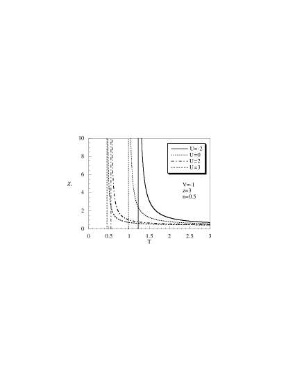
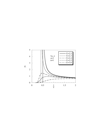
Figure 3: The charge susceptibility $\chi_{c}$ for $V=-1$ and $z=3$ as a function of the temperature $T$ for several values of $U$ and (a) $n=0.5$; (b) $n=1$.

An important quantity useful for studying the critical behavior of the system is the susceptibility. In Figs. 3, we plot the charge susceptibility as a function of the temperature for $n=0.5$ and $n=1$, and for several values of the on-site potential. From Fig. 3a, one observes that there is a critical temperature - depending on $n$ and $U$ - at which the charge susceptibility $\chi_{c}$ diverges, for both attractive and repulsive $U$. Below $T_{c}$, $\chi_{c}$ becomes negative (not reported in the graphs). As a result, one immediately infers that there exists a region where the system is thermodynamically unstable. At fixed $U$, the instability is observed in a particle density region $\Delta n=n_{1}\leq n\leq n_{2}$, whose width varies with the temperature, and vanishes for $T>T_{c}$ mancini08_2 . For values of the particle density less than half filling, the divergence of the charge susceptibility is observed for all values of $U$. As it is shown in Fig. 3b, for $n=1$ and for $U>U_{c}$, no phase transition is observed: $\chi_{c}$ is well defined for all values of $T$ and vanishes in the limit $T\to 0$. It can be shown that, in the opposite limit $T\to\infty$, $\chi_{c}$ tends to a constant value which does not depend on $U$ but only on $n$ according to the law

$$\lim_{T\to\infty}\chi_{c}=n\left(1-\frac{n}{2}\right).$$

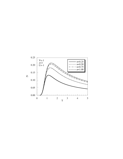
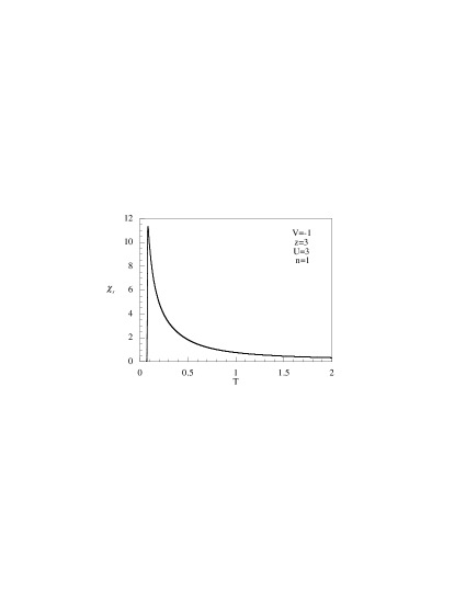
Figure 4: The spin magnetic susceptibility $\chi_{s}$ as a function of the temperature for $V=-1$ and $z=3$, and for (a) $U=-1$ and $n=0.25$, 0.5, 0.75, 1; (b) $U=3$ and $n=1$.

In Figs. 4, we plot the spin susceptibility $\chi_{s}$ as a function of the temperature. For attractive intersite interaction, at $T=T_{c}$ one does not observe substantial changes in the behavior of $\chi_{s}$. For $T>T_{c}$, the system is in the high-temperature regime and $\chi_{s}$ follows a Curie law. As it is evident from Fig. 5b, the only low-temperature region accessible to our investigation is when $n=1$ and $U>U_{c}$. In Fig. 4b, we show the spin magnetic susceptibility $\chi_{s}$ as a function of $T$ for $n=1$ and $U=3$. For $U>U_{c}$, $\chi_{s}$ is rather insensitive to the value of $U$, and a large peak is observed at low temperatures. The behavior of the spin susceptibility for repulsive intersite interactions is more relevant, as we will show in the next section, since it signals the occurrence of a CO phase.

In Fig. 5a, we report the phase diagram in the 3D space ($U,n,T$). The critical temperature $T_{c}$ and the width of the instability region $\Delta n$ increase by decreasing $U$: an attractive on-site potential will favor phase separation and in particular the clustering of doubly occupied sites. As a function of the particle density, the critical temperature shows a lobe-like behavior: it increases by increasing $n$ up to half filling, where it has a maximum; further augmenting $n$, it decreases vanishing at $n=2$. A different behavior is observed when $U>2\left|V\right|$: the lobe splits in two and $T_{c}$ increases with $n$ up to quarter filling, then decreases with a minimum at half filling. The critical temperature at $n=1$ is finite only for $U<U_{c}$. From Fig. 5b, one immediately notices that, for larger values of the on-site potential, there is no transition at half filling, as it was noticed in Ref. mancini08_2 .

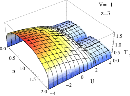
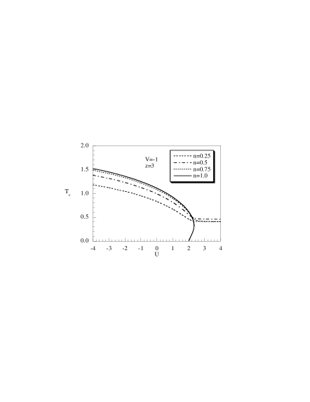
Figure 5: (a) (Color online) The critical temperature $T_{c}$ as a function of the particle density $n$ and of the on-site potential $U$ for $V=-1$ and $z=3$. (b) The critical temperature $T_{c}$ as a function of the on-site potential $U$ for $V=-1$, $z=3$ and for $n=0.25$, 0.5, 0.75, 1.

As it has been already pointed out, below the critical temperature $T_{c}$ the system is thermodynamically unstable. However, the behavior of relevant thermodynamic quantities below $T_{c}$ unveils the existence of a critical value of the on-site potential separating the two types of phase separated configurations sketched in Fig. 1 mancini08_2 . Interestingly, this critical $U$ has the same value of $U_{PS}$, turning point in the $T_{c}$-curve at half filling (see Fig. 2). In Figs. 6, we plot the double occupancy $D$, the short-range correlation function $\lambda^{(1)}$ and the internal energy $E$ as functions of $U$ for $n=0.75$ and different values of the temperature.

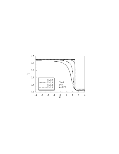
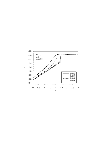
Figure 6: (a) The short-range correlation function $\lambda^{\left(1\right)}$, (b) the double occupancy $D$ and (c) the internal energy $E$ as functions of $U$ for $V=-1$, $z=3$, $n=0.75$ and for $T=0.2$, 0.3, 0.4, 0.5.

One observes that $D$ and $\lambda^{(1)}$ exhibit two plateaus at low temperatures. For $z=3$, in the limit $T\to 0$, there is a discontinuity around $U_{PS}\approx 2.3|V|$. For $U>U_{PS}$, the double occupancy vanishes, whereas $\lambda^{(1)}$ tends to $n/2$. The repulsion between the electrons on the same site and the concomitant nearest-neighbor attraction, leads to a scenario where the electrons tend to cluster together occupying neighboring sites. At half filling all sites are singly occupied, whereas for $n<1$ one observes two separated clusters of filled and empty sites. When $U<U_{PS}$, one observes a dramatic increase (step-like as $T\to 0$) of the double occupancy and of the short-range correlation function, namely: $D\to n/2$ and $\lambda^{(1)}\to n$. As a consequence, the sites are doubly occupied, and $\lambda^{(1)}=n$ indicates that the doublons (the charge carriers of doubly occupied sites) tend to occupy nearest-neighbor sites arranging to form large domains occupied, leaving the rest of the lattice empty. For $U<U_{PS}$ one also observes a dramatic decrease of the internal energy $E$, with a discontinuity as $T\to T_{c}$ around $U\approx U_{PS}$. In Figs. 7, we plot the specific heat $C$ as a function of the temperature $T$ at $n=0.75$ and for several values of the on-site potential $U$. For attractive $U$, the specific heat presents one peak whose height decreases by decreasing $U$ (see Fig. 7a). In Fig. 7b, one observes that for repulsive $U$ the height of the peak increases by increasing $U$ moving to lower temperatures. In the limit $U\to U_{PS}$, the peak becomes sharper and a divergence is observed at $U=U_{PS}$, confirming the emergence of a critical point. The same analysis carried out for different values of the particle density, evidences a similar behavior of $D$, $\lambda^{(1)}$ and $C$ as functions of $U$.

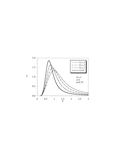
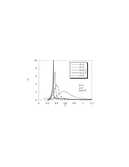
Figure 7: The specific heat $C$ as a function of the temperature $T$ for $V=-1$, $z=3$, $n=0.75$ and for (a) $U=-3$, -2, -1, 0; (b) $U=1$, 2, 2.2, 2.3, 3.

IV Repulsive intersite potential

A repulsive intersite interaction disfavors the occupation of neighboring sites. At low temperatures, this may lead to a CO phase characterized by a distribution of the electrons in alternating shells. In order to capture this phase, we shall solve the self consistent equations (38) and (39) by releasing the translational invariance requirement. To this end, one can divide the lattice into two sublattices: $A$ contains the central point ($0$) and the even shells, the sublattice $B$ contains the odd shells. Then, one requires the following boundary condition (BC) to hold:

$$\langle n(i)\rangle=\left\{{{\begin{array}[]{*{20}c}{n_{A}\hfill}\\ {n_{B}\hfill}\\ \end{array}}}\right.\quad{\begin{array}[]{*{20}c}{i\in A},\\ {i\in B},\\ \end{array}}$$ (50a)

$$n=\frac{1}{N}\sum_{i}\langle n(i)\rangle=\frac{1}{2}(n_{A}+n_{B}).$$ (50b)

Let us take two distinct sites $i\in A$ and $j\in B$. We require that the expectation values of the particle density and of the double occupancy operators at the site $i$ are equal to the ones of the neighboring sites of $j$ and viceversa, namely:

$$\begin{split}\langle n(i)\rangle&=\langle n^{\alpha}(j)\rangle,\quad\quad\langle n(j)\rangle=\langle n^{\alpha}(i)\rangle,\\ \langle D(i)\rangle&=\langle D^{\alpha}(j)\rangle,\quad\quad\langle D(j)\rangle=\langle D^{\alpha}(i)\rangle.\end{split}$$ (51)

Thus, by means of Eqs. (38) and (39), one finds two equations

$$\begin{split}&\frac{2(fF_{A}^{z}+gG_{A}^{z})}{1+2fF_{A}^{z}+gG_{A}^{z}}=\frac{1}{1+2fF_{B}^{z}+gG_{B}^{z}}\left[X_{B}\right.\\ &+\left.2fK(X_{B}+2aY_{B})F_{B}^{z-1}+gK^{2}(X_{B}+2dY_{B})G_{B}^{z-1}\right],\\ &\frac{gG_{A}^{z}}{1+2fF_{A}^{z}+gG_{A}^{z}}=\frac{Y_{B}(1+2fK^{2}F_{B}^{z-1}+gK^{4}G_{B}^{z-1})}{1+2fF_{B}^{z}+gG_{B}^{z}},\end{split}$$ (52)

plus two more equations which can be obtained by substituting $A\leftrightarrow B$. The coefficients subscripts pertain to sites belonging to the two different sublattices. In order to close the set of self-consistent equations one needs one more equation. By using the BC (50b), one can fix the particle density as

$$n=\frac{fF_{A}^{z}+gG_{A}^{z}}{1+2fF_{A}^{z}+gG_{A}^{z}}+\frac{fF_{B}^{z}+gG_{B}^{z}}{1+2fF_{B}^{z}+gG_{B}^{z}}.$$ (53)

As a result, one can now determine all the unknown parameters $X_{A}$, $X_{B}$, $Y_{A}$, $Y_{B}$, and $\mu$. By means of the same analysis employed in the previous section, one can express the local correlators $\kappa^{(p)}$ and $\lambda^{(p)}$ in terms of these parameters, and eventually compute all the properties of the system. In particular, one finds:

$$\begin{split}D&=\frac{1}{2}\left(D_{A}+D_{B}\right)\\ &=\frac{gG_{A}^{z}}{2(1+2fF_{B}^{z}+gG_{A}^{z})}+\frac{gG_{B}^{z}}{2(1+2fF_{B}^{z}+gG_{B}^{z})},\\ \lambda^{(1)}&=\frac{fK(X_{A}+2aY_{A})F_{A}^{z-1}+gK^{2}(X_{A}+2dY_{A})G_{A}^{z-1}}{1+2fF_{B}^{z}+gG_{B}^{z}}.\end{split}$$ (54)

By varying the external parameters $U$, $n$ and $T$ one has the tools to completely characterize the phase diagram pertinent to the case of repulsive intersite interactions. In the following we shall set $V=1$.

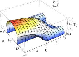
Figure 8: (Color online) (a) Phase diagram in the space ($U,n,T$) for $V=1$ and $z=3$. (b) Phase diagram in the plane ($U,T$) for $V=1$ and $z=3$ and several values of $n$.

IV.1 Phase diagram

In this section, we derive the phase diagram: by numerically solving the set of equations (52) and (53) we find a region of the $(U,n,T)$ 3D space characterized by a spontaneous breakdown of the translational invariance. In this region, shown in Fig. 8a for the case $z=3$, the population of the two sublattices $A$ and $B$ is not equivalent: the system has entered a finite temperature long-range CO phase. Upon decreasing the temperature, the distribution of the electrons becomes more and more inhomogeneous. To better understand the typology of the critical region we take sections of the 3D structure and study the 2D phase diagrams at constant $n$ in Fig. 8b and at constant $U$ in Fig. 9.

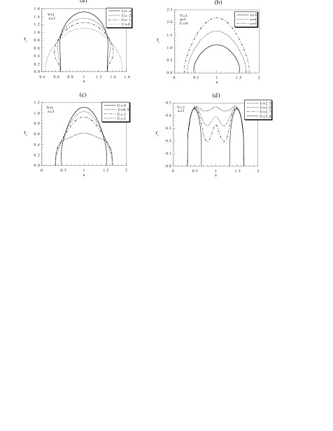
Figure 9: Phase diagram in the plane ($T,n$) for $V=1$: Figs. 9a, 9c, 9d $z=3$ and several values of $U$; Fig. 9b, $U=0$ and $z=3,4,5$.

In the plane $(U,T)$, the critical temperature line shows different behaviors according to the value of the particle density. As illustrated in Fig. 8b for the case $z=3$, one encounters the following situation. (i) For $n<1/z$ there is no CO phase for all values of $U$; (ii) For $1/z<n<n_{p}$ a CO phase is observed only for $U>0$ ($n_{p}=0.46$ for $z=3$); the critical temperature $T_{c}$ increases by increasing $U$ and tends to a constant (depending on the value of $n$) in the limit $U\to\infty$. (iii) For $n_{p}<n<2/z$ there is a CO phase for both attractive and repulsive $U$, with a reentrant behavior for $U<0$. (iv) For $n>2/z$ there is no reentrant behavior: from a constant value at large negative $U$, the critical temperature decreases by increasing $U$ and vanishes at a certain value of $U$. An interesting feature is the presence of a crossing point in the critical temperature curves around $U=2.3V$ for $z=3$. In the plane $(n,T)$, at fixed $U$, the CO phase is observed in the interval $n_{1}<n<n_{2}$; the width $\Delta=n_{2}-n_{1}$ varies with the temperature, following different laws according to the value of $U$. At $T=0$ a complete CO state is established in the regions $2/z\leq n\leq 2(z-1)/z$ for $U<0$ and $1/z\leq n\leq(2z-1)/z$ for $U>0$. For $U<0$ (see Fig. 9a), $\Delta n$ first increases with $T$, then decreases vanishing at $n=1$, where the maximum critical temperature is reached; a reentrant behavior characterizes this region. As it is shown in Fig. 9b, the value $U=0$ is a singular point; at $T=0$ the CO phase exists in the interval $n_{p}<n<2-n_{p}$. For $0<U\leq 2$ (see Fig. 9c), $\Delta n$ decreases with $T$ and no reentrant phase is observed; as in the attractive case, the phase diagram presents a single lobe structure centered at $n=1$. For $U>2$ (see Fig. 9d), one observes the formation of two lobes centered around $n=0.5$ and $n=1.5$ and the corresponding decreasing of the central lobe centered at $n=1$, which disappears at $U=U_{0}$ ($U_{0}\approx 3.7$ for $z=3$). For $U>U_{0}$ the two lobes are separated; at $T=0$ the CO phase is observed in two regions centered at $n=0.5$ and $n=1.5$. It is worthwhile to notice that for $U<2V$ and for all values of $T$ , $\Delta n$ increases by increasing the coordination number $z$; in the limit $z\to\infty$, $\Delta n\to 2$ and the CO phase is observed for all values of $n$. Besides the translational-invariance broken solution in the 3D region illustrated in Fig. 8a, the set of equations (52) and (53) admits also a homogeneous solution. In order to determine which solution is energetically favored one has to look at the free energy. The Helmholtz free energy $F$ can be computed by means of the formula

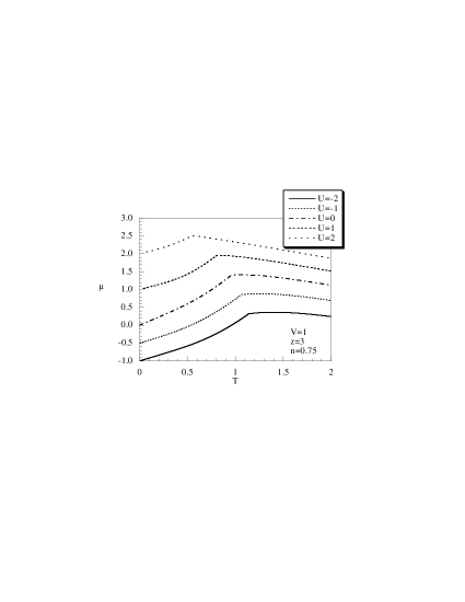
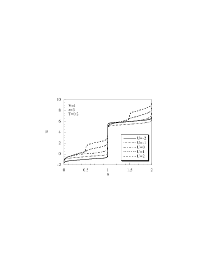
Figure 10: (a) The chemical potential $\mu$ as a function of the temperature for $V=1$, $z=3$, $n=0.75$ and different on-site interactions. (b) The chemical potential $\mu$ as a function of the particle density $n$ for $z=3$, $T=0.2$ and various on-site interactions.

$$F(T,n)=\int\limits_{0}^{n}\mu(T,n^{\prime})dn^{\prime}.$$

Upon defining the difference $\Delta F=F_{hom}-F_{CO}$ - where $F_{hom}$ is the free energy of the homogeneous phase and $F_{CO}$ the one of the CO phase, respectively - one finds that below the transition temperature the CO phase is energetically favored since $\Delta F\geq 0$. In particular, $\Delta F$ smoothly vanishes for $T\to T_{c}$, signalling a second-order phase transition.

IV.2 Thermodynamic properties

In this section, we shall determine several thermodynamic quantities whose behaviors support the scenario depicted in the previous section. The behavior of the chemical potential as a function of the temperature and of the particle density $n$ is reported in Figs. 10a and 10b, respectively. One can immediately notice that, as a function of the temperature, $\mu$ presents a cuspid at $T=T_{c}$: for $T\geq T_{c}$ ($T\leq T_{c}$) $\mu$ is a decreasing (increasing) function of $T$. When plotted at fixed temperature, the chemical potential is always an increasing function of $n$, hinting at a thermodynamically stable system, for both the CO and homogeneous phases. In the limit $T\to 0$, $\mu$ shows two plateaus for $U<2V$ in the range $0<n\leq 2$; when $U>2V$ each plateau splits in two sub-plateaus.

A full comprehension of the phase diagram and of the distribution of the particles on the sites of the Bethe lattice can be achieved by a detailed investigation of the particle density and of the double occupancy. In particular, the study of the different contributions coming from the two sublattices, reveals the onset of CO states, the reentrant behavior, and also the distribution of the electrons in the shells of the Bethe lattice. In Figs. 11a and 11b, we plot the sublattices variables $n_{A}$ and $n_{B}$ as functions of the temperature for $n=0.5$, $n=0.75$, and several values of $U$.

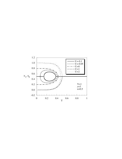
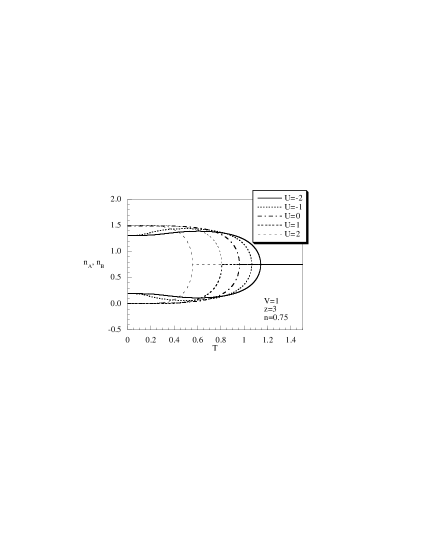
Figure 11: The sublattices variables $n_{A}$ and $n_{B}$ as functions of the temperature for $V=1$, $z=3$, several values of $U$ and: (a) $n=0.5$, (b) $n=0.75$.

At high temperatures the particles distribute homogeneously in the entire lattice: $n_{A}=n_{B}=n$. Upon lowering the temperature, one finds that at the critical temperature $T_{c}=T_{c}(n,U)$ a CO phase is established; the particles tend to fill one sublattice ($B$) and to empty the other sublattice ($A$). By further lowering the temperature, the behavior is different according to the values of $n$ and $U$. For $n=0.5$, one observes the following situation: (i) for $U$ negative and close to zero the phase diagram exhibits a reentrant behavior (see Fig. 8b); correspondingly, as shown in Fig. 11a, there is another critical temperature at which the translational invariance is restored and the two sublattices are again equally populated; (ii) for $U=0$, the anisotropy of the filling increases and, at $T=0$, one finds $n_{A}=2n/5$ and $n_{B}=8n/5$ for $z=3$; (iii) for $U>0$ a total charge order is established in the limit $T\to 0$: all the particles reside in one sublattice ($B$) whilst the other is completely empty. For $n=0.75$ and $n=1$ (not shown), there is no reentrant phase; by lowering $T$, $n_{A}$ ($n_{B}$) decreases (increases) and tends to zero (2$n$) at $T=0$ (for $n=0.75$ and $U<0$ charge ordering is not complete, since a small fraction of particles is found in the sublattice $A$, also at $T=0$).

In Figs. 12a and 12b, we plot the sublattice double occupancies $D_{A}$ and $D_{B}$ as functions of the temperature for $n=0.5$ and $n=0.75$ and several values of $U$. At high temperatures the system is in a homogeneous phase and, correspondingly $D_{A}=D_{B}=D$. Upon lowering the temperature, one finds that at $T_{c}$ there is a phase transition to a CO state: $D_{B}$ increases while $D_{A}$ decreases. By further lowering the temperature, one observes different behaviors according to the values of $n$ and $U$. A reentrant phase characterized by a second critical temperature at which the system returns to the homogeneous phase where the double occupancy tends to $n/2$ in the two sublattices (observed for $n=0.5$ and $U$ negative and small). The CO persists in the limit $T\to 0$ with: (i) $D_{A}$ and $D_{B}$ both vanishing at $T=0$ (observed for $n=0.5$ and $U>0$); (ii) $D_{A}$ ($D_{B}$) decreases (increases) and tends to a finite value (observed for $n=0.75$ and $U<0$); (iii) $D_{A}$ ($D_{B}$) decreases (increases) and tends to zero ($n$) (observed for $n=0.75$, $U>0$ and $n=1$, $\forall U$).

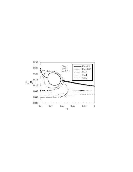
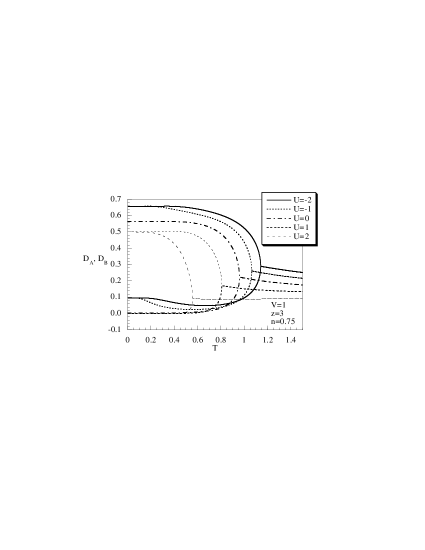
Figure 12: The sublattices variables $D_{A}$ and $D_{B}$ as functions of the temperature as functions of the temperature for $V=1$, $z=3$, several values of $U$ and: (a) $n=0.5$, (b) $n=0.75$.

Since the specific heat exhibits a very rich structure in correspondence to the critical lines in the phase diagram shown in Fig. 8a, we shall investigate its behavior for different values of the particle density $n$. The possible excitations of the ground state are creation and annihilation of singly occupied or doubly occupied states, induced by the Hubbard operators $\psi^{(\xi)}$ and $\psi^{(\eta)}$, respectively mancini08_PRE . The corresponding transition energies are given in Eqs. (13) and the high and low temperature peaks exhibited by the specific heat are due to these transitions. One may distinguish between them by looking at the position of the peaks, i.e., if the position changes or remains constant by varying $U$. Besides these peaks, one also observes peaks in correspondence to the transition temperatures separating homogeneous and CO phases. Of course, in the case of a reentrant phase, one correspondingly observes two peaks relative to the transitions.

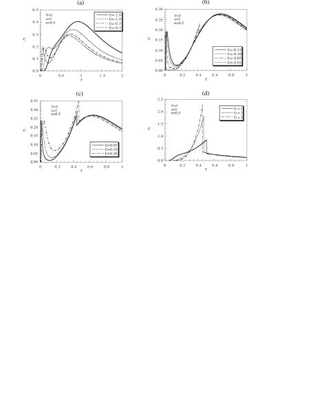
Figure 13: (a) The specific heat as a function of the temperature for $z=3$, $V=1$, $n=0.5$ and different regions of $U$: (a) attractive interaction $U=-2,\ldots,-0.3$; (b) $U$ negative and close to zero; (c) $U$ positive and close to zero; (d) $U$ large and positive.

The behavior of the specific heat at $n=0.5$ as a function of the temperature is shown in Figs. 13a-d. For $U$ negative and large ($U=-3V,-2V$), there is no CO and $C$ exhibits only one peak at high temperature at position $T_{1}\approx 1$; by increasing $U$ ($U=-V$, $-0.5V$, $-0.3V$) a second peak appears at low temperatures $T_{2}\approx 0.1$ and the position of the first peak decreases (see Fig. 13a). Further increasing $U$, a reentrant phase transition from the homogeneous phase to the CO state occurs; correspondingly, two new peaks are observed around the two critical temperatures $T_{3}\approx 0.4$ and $T_{4}\approx 0.15$ (see Fig. 13b). For attractive on-site interactions the possible excitations are creation and annihilation of doubly occupied states, and the charge peaks at $T_{1}$ and $T_{2}$ are mainly induced by $\psi^{(\eta)}$; these peaks move towards low temperatures, with $T_{2}\to 0$ as $U\to 0$. For $U$ small and positive and close to zero, there is a phase transition but no reentrant phase, $T_{3}=0$. The specific heat exhibits a three-peak structure (see Fig. 13c): one peak at high temperature ($T_{1}\approx 0.7$), a second peak at low temperatures ($T_{2}\approx 0.02$), and a third peak around $T_{3}\approx 0.4$. For $U$ positive and large (see Fig. 13d) only one peak at $T_{3}\approx 0.5$ appears due to the phase transition to the CO state. The behavior of the specific heat at $n=0.75$ as a function of the temperature is shown in Figs. 14a-c. For $n=0.75$ there is no reentrant behavior. At low temperatures the system is in a CO state and exhibits a phase transition at $T_{c}$ to a homogeneous phase.

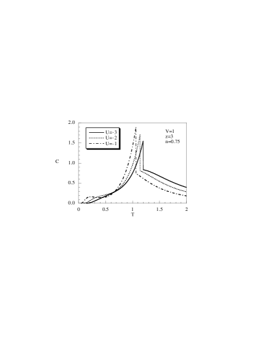
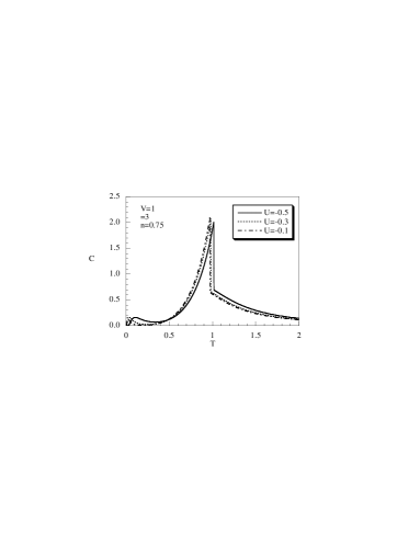
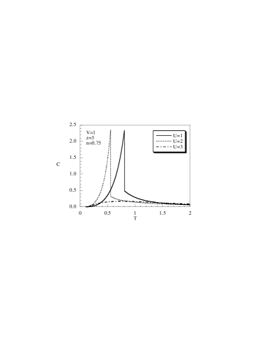
Figure 14: The specific heat as a function of the temperature for $z=3$, $V=1$, $n=0.75$ and different regions of $U$: (a) large attractive interaction $U=-2,\ldots,-1$; (b) $U$ negative and close to zero; (c) $U$ large and positive.

For $U$ negative and large only one peak appears at $T_{3}=T_{c}$, due to the phase transition. For $U$ negative and small, besides the peak at $T_{3}$, one observes another peak $T_{2}$ at low temperatures which vanishes as $U$ approaches zero. For $0\leq U<3V$, there is only one peak at $T_{3}=T_{c}$; contrarily to the case of $n=0.5$, the peak $T_{2}$ is not observed for $U$ positive. For $U\geq 3V$ ($z=3)$ there is no phase transition and one broad peak of much more intensity is observed. The behavior of the specific heat at half filling as a function of the temperature is shown in Figs. 15a-b. For $n=1$, a CO phase is observed for all values of $U<U_{0}$. As it is shown in Fig. 15a, the specific heat exhibits one peak situated at $T_{3}=T_{c}$ moving towards low temperatures as $U$ increases. At $T=0$, for $U<U_{0}$, one sublattice ($A$) is empty, whereas the other sublattice ($B$) has all sites doubly occupied; there are neither singly occupied sites nor neighbor sites occupied ($\lambda^{(1)}=0$). The energy of the ground state is non-degenerate. For $U>U_{0}$, one observes a homogeneous state: all sites are singly occupied and the energy of the ground state is infinitely degenerate since the spins are arbitrarily oriented.

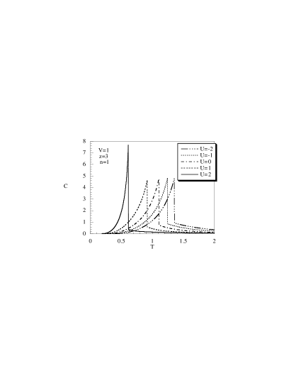
Figure 15: The specific heat as a function of the temperature for $z=3$, $V=1$, $n=1$ and different regions of $U$: (a) values of $U$ far from the critical point $U_{0}$; (b) values of $U$ approaching $U_{0}$.

At $T=0$ and $U=U_{0}$, there is a phase transition from a non-degenerate level to a degenerate one; therefore one expects a discontinuity in the internal energy $E$ and, correspondingly, a divergence in the specific heat in the limit $U\to U_{0}$. This is clearly observed in Fig. 15b.

Other important quantities, useful for studying the critical behavior of the system, are the charge and spin susceptibilities. In fact, anomalies in their behaviors clearly signal the onset of a CO state. The charge susceptibility can be defined separately for the two sublattices:

$$\chi_{c}^{A}=\frac{\partial n_{A}}{\partial\mu},\quad\quad\quad\chi_{c}^{B}=\frac{\partial n_{B}}{\partial\mu},$$

where the total charge susceptibility is given by $\chi_{c}=\left(\chi_{c}^{A}+\chi_{c}^{B}\right)/2$.

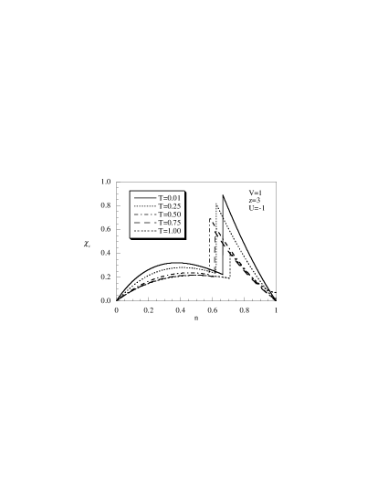
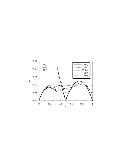
Figure 16: The charge susceptibility as a function of the particle density for $z=3$, $V=1$, different values of the temperatures and (a) $U=-1$; (b) $U=2.1$.

By studying separately $\chi_{c}^{A}$ and $\chi_{c}^{B}$, it is manifest their different contribution to the total charge susceptibility. By varying the particle density at fixed (low) temperature, one finds a critical value of the particle density ($n_{c}$) at which the susceptibilities $\chi_{c}^{A}$ and $\chi_{c}^{B}$ show a discontinuity: below $n_{c}$, one finds $\chi_{c}^{A}=\chi_{c}^{B}=\chi_{c}$, whereas above $n_{c}$ one observes the depletion of sublattice $A$ and the corresponding accumulation of the particles in the sublattice $B$. For $n>n_{c}$, the susceptibility $\chi_{c}^{A}$ becomes negative, since $n_{A}$ is a decreasing function of $n$. As a result, the system is in a CO phase with “almost empty” shells separated by filled shells. Of course, at half filling and in the limit $T\to 0$, one finds $n_{A}=0$ and $n_{B}=2$ and the susceptibility vanishes. In Fig. 16, we plot the charge susceptibility as a function of the particle density for a given value of $U$ and several values of the temperature. At low temperatures, $\chi_{c}$ shows a quasi-one or -two lobe structure, depending on the value of the on-site potential. For $z=2$, i.e., a 1D chain, the lobes have a regular shape mancini08_PRE . For $z\geq 3$, the curvature of the lobes is different above and below $n_{c}$ and the observed discontinuity signals the transition to a phase where translational invariance is broken. The vanishing of $\chi_{c}$ for $T\to 0$ at quarter and half filling indicates that a full CO state is established. In Figs. 17a-b, we plot $\chi_{c}$ as a function of the temperature, for $U=V$ and $U=2.1V$, and for different values of the filling ($n=0.25$, 0.5, 0.75, 1).

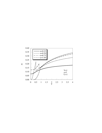
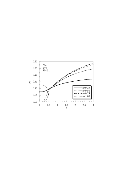
Figure 17: The charge susceptibility $\chi_{c}$ as a function of the temperature for $z=3$, $V=1$, $n=0.25$, 0.5, 0.75, 1 and (a) $U=1$, (b) $U=2.1$.

For $n=0.25$ there is no charge ordering and one finds $\chi_{c}^{A}=\chi_{c}^{B}=\chi_{c}$. At $n=0.5$ and $n=0.75$, the system is in a CO phase characterized by a different filling of the shells for $T<T_{c}$: as a consequence, $\chi_{c}^{A}\neq\chi_{c}^{B}$, and $\chi_{c}$ presents a discontinuity. At half filling, there is charge ordering but the susceptibility is the same in the two sublattices, also for $T<T_{c}$. The limit $T\to 0$ of the charge susceptibility dramatically depends on the value of the particle density: $\chi_{c}$ is finite for values of the particle density corresponding to translational invariant states, whereas it decreases with $T$ and vanishes for fillings corresponding to CO states characterized by alternating empty and filled shells. In the limit of high temperatures, the charge susceptibility tends to a constant value which does not depend on $U$ and $z$ but only on $n$ according to the law mancini08_PRE

$$\lim_{T\to\infty}\chi_{c}=\alpha(n),$$ (55)

where $\alpha(n)=n(2-n)/2$.

The spin magnetic susceptibility $\chi_{s}$ in zero field, given in Eq. (41), can also be defined separately for the two sublattices. In Figs. 18a-b we plot the spin susceptibilities $\chi_{s}$, $\chi_{s}^{A}$ and $\chi_{s}^{B}$ as functions of the temperature for two representative values of $U$ ($U=-V$ and $U=2.1V$, respectively) and for different values of the filling. For $U=-V$, the spin susceptibility vanishes at zero temperature for all values of the filling: all the electrons are paired and no alignment of the spin is possible. By increasing $T$, the thermal excitations break some of the doublons and a small magnetic field may induce a finite magnetization: $\chi_{s}$ augments by increasing $T$ up to a maximum, which might be different for the two sublattices, then decreases. For $n=0.25$ and $n=0.5$ the system is not charge ordered and $\chi_{s}$ has the same value in the two sublattices. Conversely, for $n=0.75$ and $n=0.9$ the system is charge ordered when $T<T_{c}$: $\chi_{s}$ assumes different values in the two sublattices.

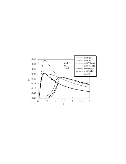
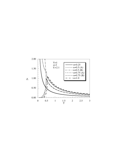
Figure 18: (a) The spin susceptibilities $\chi_{s}$, $\chi_{s}^{A}$ and $\chi_{s}^{B}$ as a function of the temperature for $V=1$, $n=0.25$, 0.5, 0.75, 1 and for (a) $U=-1$ and (b) $U=2.1$.

For $U=2.1V$, when the system is not charge ordered, $\chi_{s}^{A}=\chi_{s}^{B}=\chi_{s}$ diverges for $T\to 0$, whereas for CO states $\chi_{s}^{A}$ vanishes and $\chi_{s}^{B}$ diverges in the same limit. At low temperatures, only the electrons belonging to sublattice $A$ are paired and, as a consequence, $\chi_{s}^{A}=0$. At half filling, for both $U=-V$ and $U=2.1V$, even in the presence of charge ordering, $\chi_{s}$ has the same value in the two sublattices $A$ and $B$. It is easy to check that, for high temperatures, the spin susceptibility decreases with the Curie law: $\lim_{T\to\infty}\chi_{s}=\alpha(n)/T$ in the entire ($U,n$) plane, where $\alpha(n)$ is the same $z$ and $U$ independent function appearing in Eq. (55) mancini08_PRE . As a consequence, in the limit of high temperatures, the ratio $\chi_{c}/\chi_{s}$ is an universal function of $T$, namely: $\lim_{T\to\infty}\left(\chi_{c}/\chi_{s}\right)=T$.

To conclude this section, we report some results obtained for the entropy as a function of $T$, and $U$, showing that also this quantity is a good indicator of the onset of a CO state. The standard way to compute the entropy is by integrating via the integral of the specific heat:

$$S(T)=S(0)+\int_{0}^{T}\frac{C(T)}{T}\,dT.$$

However, as extensively commented on in Ref. mancini08_PRE , this expression can not be easily handled since it requires the calculation of $S(0)$, which is generally not an easy task. A more convenient formula is given by:

$$S(n,T,U)=-\int_{0}^{n}\frac{\partial\mu(n^{\prime},T,U)}{\partial T}\,dn^{\prime}.$$

In our framework of calculations, we can readily deal with this expression since it requires only the knowledge of the chemical potential. In Figs. 19a and 19b we plot the entropy as a function of the temperature for $n=0.5$ and $n=1$, respectively.

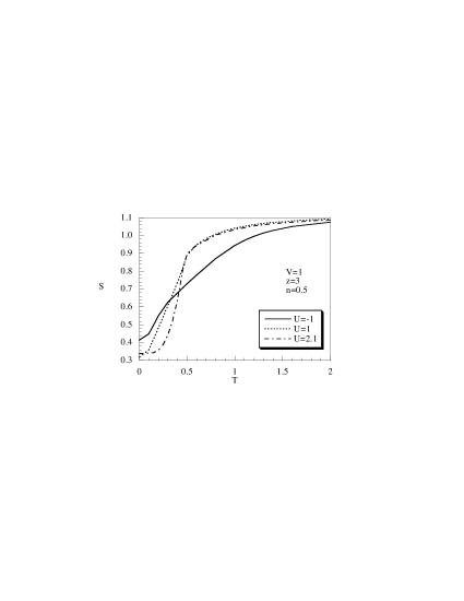
Figure 19: The entropy $S$ as a function of the temperature for $z=3$, $V=1$, $U=-1$, 1, 2.1 and (a) $n=0.5$, (b) $n=1$.

One can notice an abrupt change of the entropy curves when the critical temperature is reached. One may also notice that, in the limit $T\to 0$, $S(0)$ is finite for $n=0.5$ due to the degeneracy of the ground state energy. On the other hand, $S(0)$ is zero at half filling because there is no degeneracy of the ground state. The $U$ dependence of the entropy is rather dramatic in the neighborhood of the values at which a zero temperature transition occurs, as it is evident from Fig. 20. At low temperatures, the entropy presents a step-like behavior and becomes rather insensitive to variations in $U$ for sufficiently large on-site repulsive and attractive interactions. For $0<n<1/z$, one observes an increase of the entropy at $U=0$ in the limit $T\to 0$: even if there is no transition, there is a change of the distribution of the electrons from a configuration characterized by doubly occupied sites to one with singly occupied sites, which is less ordered. When $1/z<n<2/z$, the entropy presents a discontinuity around $U=0$ (due to the phase transition) which becomes more pronounced as the temperature decreases. In the region $2/z<n<1$, at low temperatures, one finds a rather sharp increase of the entropy near $U_{0}(n)$, where the system undergoes a transition from a CO phase to a translational invariant state, less ordered.

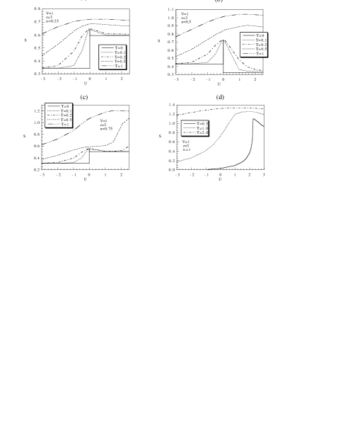
Figure 20: The entropy $S$ as a function of $U$ for $z=3$, $V=1$, for temperatures varying in the interval (0,1) and (a): $n=0.25$, (b): $n=0.5$, (c): $n=0.75$, (d): $n=1$.

V concluding remarks

Statistical models on the Bethe lattice are of considerable interest since they admit a direct analytical approach for a number of problems that may be otherwise intractable on Euclidean lattices. In this paper, we have evidenced how the use of the Green’s function and equations of motion formalism leads to the exact solution of the extended Hubbard model on the Bethe lattice in the narrow-band limit. We provided a comprehensive and systematic analysis of the model by considering relevant thermodynamic quantities in the whole space of the parameters $n$, $T$, $U$ and $V$ and we obtained the finite temperature phase diagram, for both attractive and repulsive on-site and intersite interactions.

The phase diagram dramatically depends on the sign of the nearest-neighbor interaction. In the attractive case, there is a critical temperature $T_{c}$, located by the divergence of the charge susceptibility, at which there is a transition from a thermodynamically stable to an unstable phase; the latter is characterized by phase separation. The surface separating the two phases has a rounded vault in the 3D ($n$, $U$, $T$) space, which splits in two for $U>U_{c}(z)$. Below $T_{c}$, the same critical value of the on-site potential separates the two possible configurations of phase separated states, namely clusters of singly or doubly occupied sites. For repulsive nearest-neighbor interactions, the phase diagram has a richer structure: we found a transition temperature below which translational invariance is broken. The Bethe lattice effectively splits in two sublattices with different thermodynamic properties. As a result, a charge ordered phase, characterized by a different distribution of the electrons in alternating shells, is established for $n>1/z$. The CO phase is energetically favored as demonstrated by the study of the Helmholtz free energy. By investigating the behavior of several thermodynamic quantities, we attained a full comprehension of the phase diagram. The study of the particle density and of the double occupancy is particularly enlightening to unveil the distribution of the particles on the sites of the Bethe lattice. The specific heat exhibits not only high and low temperature peaks due to charge excitations induced by the Hubbard operators $\psi^{(\xi)}$ and $\psi^{(\eta)}$, but also peaks due to the phase transition from the homogeneous phase to the CO state (or viceversa). By studying separately the contribution to the charge and spin susceptibilities coming from the two sublattices, the onset of a CO phase is also signalled by the separation of the values of the sublattices quantities $\chi_{c,s}^{A}$ and $\chi_{c,s}^{B}$ . The different population of the two sublattices in the CO phase is reflected by the divergence or the vanishing, in the limit $T\to 0$, of the spin susceptibilities $\chi_{s}^{A}$ and $\chi_{s}^{B}$. If the electrons are paired, no alignment of the spin is possible ($\chi_{s}^{A}\to 0$), whereas single occupation of the sites leads to an alignment ($\chi_{s}^{B}\to\infty$) even when the magnetic field is turned off.

Appendix A The extended Hubbard model on the Bethe lattice in the presence of an external magnetic field

In the presence of an external magnetic field $h$, the Hamiltonian of the AL-EHM reads:

$$\begin{split}H&=-\mu\sum_{i}n(i)+U\sum_{i}D(i)\\ &+\frac{1}{2}\sum_{i\neq j}V_{ij}n(i)n(j)-h\sum_{i}n_{3}(i),\end{split}$$ (56)

where $n_{3}(i)$ is the third component of the spin density operator

$$n_{3}(i)=n_{\uparrow}(i)-n_{\downarrow}(i)=c_{\uparrow}^{\dagger}(i)c_{\uparrow}(i)-c_{\downarrow}^{\dagger}(i)c_{\downarrow}(i).$$ (57)

The formulation given in Section II for the case of a Bethe lattice must be generalized in order to take into account the breaking of rotational invariance in the spin space: one has to distinguish the two components - in the spinorial notation - of the fermionic fields. By exploiting the decomposition (25), it is not difficult to show that the presence of the magnetic field affects only $H_{0}$. In this representation the equations of motion of the Hubbard operators become

$$\begin{split}\left[\xi_{\sigma}(i),H_{0}\right]&=-\left(\mu+\sigma h\right)\xi_{\sigma}(i),\\ \left[\eta_{\sigma}(i),H_{0}\right]&=-\left(\mu+\sigma h-U\right)\eta_{\sigma}(i),\end{split}$$ (58)

and Eqs. (38) are modified as:

$$\begin{split}\langle n_{\uparrow}(i)\rangle_{0}&=\frac{e^{\beta(\mu+2h)}+e^{\beta(2\mu+h-U)}}{e^{\beta h}+e^{\beta\mu}+e^{\beta(\mu+2h)}+e^{\beta(2\mu+h-U)}},\\ \langle n_{\downarrow}(i)\rangle_{0}&=\frac{e^{\beta\mu}+e^{\beta(2\mu+h-U)}}{e^{\beta h}+e^{\beta\mu}+e^{\beta(\mu+2h)}+e^{\beta(2\mu+h-U)}},\\ \langle D(i)\rangle_{0}&=\frac{e^{\beta(2\mu+h-U)}}{e^{\beta h}+e^{\beta\mu}+e^{\beta(\mu+2h)}+e^{\beta(2\mu+h-U)}},\\ \langle n_{3}(i)\rangle_{0}&=\frac{e^{\beta\mu}(e^{2\beta h}-1)}{e^{\beta h}+e^{\beta\mu}+e^{\beta(\mu+2h)}+e^{\beta(2\mu+h-U)}}.\end{split}$$ (59)

All the rest of formulation developed in Sections II, III and IV follows easily. It is worth noticing that the magnetization takes the simple expression:

$$\langle n_{3}(i)\rangle=\tanh(\beta h)[\langle n(i)\rangle-2\langle D(i)\rangle].$$ (60)

References

- (1) F. Mancini and F. P. Mancini, Phys. Rev. E 77, 061120 (2008).
- (2) F. Mancini, F. P. Mancini, and A. Naddeo, J. Opt. Adv. Mat. 10, 1688 (2008).
- (3) F. Mancini, F. P. Mancini, and A. Naddeo, Eur. Phys. J. B 68, 309 (2009).
- (4) R. J. Baxter, Exactly Solvable Models in Statistical Mechanics, Academic Press, New York (1982).
- (5) C. Kwon and D. J. Thouless, Phys. Rev. B 43, 8379 (1991); J. L. Monroe, Phys. Lett. A 188, 80 (1994); P. D. Gujrati, Phys. Rev. Lett. 74, 809 (1995).
- (6) M. Eckstein, M. Kollar, M. Potthoff, and D. Vollhardt, Phys. Rev. B 75, 125103 (2007).
- (7) R. Peters and T. Pruschke, Phys. Rev. B 79, 045108 (2009).
- (8) I. Cuadrado, M. Moran, C. M. Casado, B. Alonso, and J. Losada, Coordin. Chem. Rev. 193, 395 (1999).
- (9) K. Inoue, Prog. Polym. Sci. 25, 453 (2000).
- (10) Special issue on optical properties of dendrimers, J. Lumin. 111, 215 (2005).
- (11) F. Mancini and A. Avella, Adv. Phys. 53, 537 (2004).
- (12) L. Onsager, Phys. Rev. 65, 117 (1944).
- (13) F. Mancini, Europhys. Lett. 70, 485 (2005).
- (14) F. Mancini, Eur. Phys. J. B 45, 497 (2005).
- (15) F. Mancini and A. Naddeo, Phys. Rev. E 74, 061108 (2006).
- (16) A. Avella and F. Mancini, Eur. Phys. J. B 50, 527 (2006).
- (17) F. Mancini and F. P. Mancini, Condens. Matt. Phys. 11, 543 (2008).
- (18) J. E. Hirsch, E. Loh, Jr., D. J. Scalapino, and S. Tang, Phys. Rev. B 39, 243 (1989).
- (19) P. G. J. van Dongen, Phys. Rev. Lett 74, 182 (1995).
- (20) H. Q. Lin, D. K. Campbell, and R. T. Clay, Chinese J. Phys. 38, 1 (2000).
- (21) N.-H. Tong, S.-Q. Shen, and R. Bulla, Phys. Rev. B 70, 085118 (2004).
- (22) R. Pietig, R. Bulla, and S. Blawid, Phys. Rev. Lett 82, 4046 (1999).
- (23) A. T. Hoang and P. Thalmeier, J. Phys.: Condens. Matter 14, 6639 (2002).
- (24) H. Seo, J. Merino, H. Yoshioka, and M. Ogata, J. Phys. Soc. Jap. 75, 051009 (2006).
- (25) G. Pawłowski, Eur. Phys. J. B 53, 471 (2006).
- (26) D. Baeriswyl, D. K. Campbell, and S. Mazumdar in Conjugated Conducting Polymers, edited by H. Kiess (Springer, Berlin, 1992), pp. 7-134.
- (27) F. Mancini, Eur. Phys. J. B 47, 527 (2005).