Qubit dynamics in a $q$-deformed oscillators environment

Sonia L’Innocente Dipartimento di Matematica & Informatica, UniversitΓ  di Camerino, I-62032 Camerino, Italy    Cosmo Lupo Dipartimento di Fisica, UniversitΓ  di Camerino, I-62032 Camerino, Italy    Stefano Mancini Dipartimento di Fisica, UniversitΓ  di Camerino, I-62032 Camerino, Italy INFN, Sezione di Perugia, I-06123 Perugia, Italy
Abstract

We study the dynamics of one and two qubits plunged in a $q$-deformed oscillators environment. Specifically we evaluate the decay of quantum coherence and entanglement in time when passing from bosonic to fermionic environments. Slowing down of decoherence in the fermionic case is found. The effect only manifests at finite temperature.

I Introduction

Open system dynamics is of uppermost importance in the quantum regime where non classical phenomena turn out to be very fragile with respect to any noise source. The noise effects are often modeled as the result of an interaction of the system with a large number of uncontrollable degrees of freedom, i.e.Β an environment gardiner . Environments can be assumed as to be composed by different kinds of particles, for instance oscillators or spin-$\frac{1}{2}$. These objects come, under the mathematical point of view, from the realizations of two different algebras (the Heisenberg-Weyl algebra and the Lie algebra su$(2)$) corresponding to fermionic and bosonic commutation relations. These latter can be seen as two limit cases of more general commutation relations involving deformed algebras parameterized by one continuous parameter Kury ; Kulish ; Mac .

Our aim is to analyze the qubit dynamics in an environment of oscillators satisfying suitable $q$-deformed commutation relations, such that it permits to continuously interpolate between oscillators and spin-$\frac{1}{2}$. Actually, we investigate how quantum decoherence phenomena changes in passing from bosonic to fermionic environments. We find a slowing down of decoherence in the fermionic case. However, this effect only manifests at finite temperature.

The paper is organized as follows. In Section II we present the model. We then derive the master equation in Section III. In Section IV we study the dynamics of a single qubit and we evaluate its coherence decay. We then study the dynamics of two qubits and we evaluate the entanglement decay by distinguishing the case of the two qubits in the same environment (Section V), from that of the two qubits in separate environments (Section VI). Finally, Section VII is for concluding remarks.

II The model

Let us consider a system (qubit) described by the free Hamiltonian

$\displaystyle H_{S}$ $\displaystyle=$ $\displaystyle\Omega\sigma_{z},$ (1)

with $\Omega$ the qubit frequency and $\sigma$, σ†superscriptπœŽβ€ \sigma^{{\dagger}}, $\sigma_{z}$ operators satisfying the commutation relations

[σ†,Οƒ]superscriptπœŽβ€ πœŽ\displaystyle\left[\sigma^{{\dagger}},\sigma\right] $\displaystyle=$ $\displaystyle\sigma_{z},$ (2)
$\displaystyle\left[\sigma,\sigma_{z}\right]$ $\displaystyle=$ $\displaystyle 2\sigma,$ (3)
[σ†,Οƒz]superscriptπœŽβ€ subscriptπœŽπ‘§\displaystyle\left[\sigma^{{\dagger}},\sigma_{z}\right] $\displaystyle=$ βˆ’2​σ†.2superscriptπœŽβ€ \displaystyle-2\sigma^{{\dagger}}. (4)

They define the su$(2)$ algebra. Furthermore, we consider an environment composed by an infinite (countable) number of oscillators whose Hamiltonian reads as Greenberg ; Ham1

$\displaystyle H_{E}$ $\displaystyle=$ $\displaystyle\sum_{k}\omega_{k}N_{k},$ (5)

with $\omega_{k}$ the frequency of the $k$-th oscillator and $A_{k}$, Ak†superscriptsubscriptπ΄π‘˜β€ A_{k}^{\dagger}, $N_{k}$ operators satisfying the commutation relations

$\displaystyle{[}N_{h},A_{k}{]}$ $\displaystyle=$ $\displaystyle-\delta_{hk}A_{k},$ (6)
[Nh,Ak†]subscriptπ‘β„Žsubscriptsuperscriptπ΄β€ π‘˜\displaystyle{[}N_{h},A^{\dagger}_{k}{]} $\displaystyle=$ Ξ΄h​k​Ak†.subscriptπ›Ώβ„Žπ‘˜subscriptsuperscriptπ΄β€ π‘˜\displaystyle\delta_{hk}A^{\dagger}_{k}. (7)

They define the Heisenberg-Weyl algebra. We are now going to introduce a deformation of this algebra through the so-called β€œquons” commutation relations Greenberg

Ah​Akβ€ βˆ’q​Ak†​Ah=Ξ΄h​k,subscriptπ΄β„Žsuperscriptsubscriptπ΄π‘˜β€ π‘žsuperscriptsubscriptπ΄π‘˜β€ subscriptπ΄β„Žsubscriptπ›Ώβ„Žπ‘˜A_{h}A_{k}^{\dagger}-qA_{k}^{\dagger}A_{h}=\delta_{hk}, (8)

where $q\in[-1,1]$ is the deformation parameter. It allows us to interpolate between fermions ($q=-1$) and bosons ($q=1$). Intermediate values of $q\in(-1,1)$ correspond to the so-called β€œinfinite statistics”.

We assume the system interacting with the environment through the following Hamiltonian

$\displaystyle H_{I}$ $\displaystyle=$ βˆ‘kΞ»k​(Ak†​σ+Ak​σ†),subscriptπ‘˜subscriptπœ†π‘˜subscriptsuperscriptπ΄β€ π‘˜πœŽsubscriptπ΄π‘˜superscriptπœŽβ€ \displaystyle\sum_{k}\lambda_{k}\left(A^{{\dagger}}_{k}\sigma+A_{k}\sigma^{{\dagger}}\right), (9)

where $\lambda_{k}$ denotes the coupling constant of the system with the $k$-th environment’s oscillator.

III Master Equation

Quite generally, the master equation for the system density operator $\rho$ can be derived by using the Born-Markov approximation gardiner . Hence, it can be formally written as

$$\dot{\rho}(t)=-\int_{0}^{\infty}d\tau{\rm Tr}_{E}\left\{\left[H_{I}(t),\left[H_{I}(t-\tau),\rho(t)\otimes\rho_{E}\right]\right]\right\},$$ (10)

where $\rho_{E}$ is the initial environment density operator and ${\rm Tr}_{E}$ denotes the trace over environment degrees of freedom. Furthermore, it is

$$H_{I}(t)=e^{\iota(H_{S}+H_{E})t}H_{I}e^{-\iota(H_{S}+H_{E})t}.$$ (11)

For the choice of the environment Hamiltonian (5), the dynamical equations are formally identical to the undeformed case. The reason is that the interaction Hamiltonian $H_{I}(t)$ reads as follows

HI​(t)=βˆ‘kΞ»k​(Ak†​σ​eβˆ’ΞΉβ€‹(Ο‰kβˆ’Ξ©)​t+Ak​σ†​eι​(Ο‰kβˆ’Ξ©)​t),subscript𝐻𝐼𝑑subscriptπ‘˜subscriptπœ†π‘˜subscriptsuperscriptπ΄β€ π‘˜πœŽsuperscriptπ‘’πœ„subscriptπœ”π‘˜Ξ©π‘‘subscriptπ΄π‘˜superscriptπœŽβ€ superscriptπ‘’πœ„subscriptπœ”π‘˜Ξ©π‘‘H_{I}(t)=\sum_{k}\lambda_{k}\left(A^{{\dagger}}_{k}\sigma e^{-\iota(\omega_{k}-\Omega)t}+A_{k}\sigma^{{\dagger}}e^{\iota(\omega_{k}-\Omega)t}\right), (12)

by virtue of (11), (9), (5) and (1). Therefore, from (10), we can write

$$\dot{\rho}(t)=-\int_{0}^{\infty}d\tau{\rm Tr}_{E}\sum_{k,l}\lambda_{k}\lambda_{l}\mathcal{F}_{kl}(\rho(t)),$$ (13)

where

$\displaystyle\mathcal{F}_{kl}(\rho(t))\,=\,$ $\displaystyle F_{k}(t)\,F_{l}(t-\tau)\,\rho(t)\otimes\rho_{E}-F_{k}(t)\,\rho(t)\otimes\rho_{E}\,F_{l}(t-\tau)$
$\displaystyle-F_{k}(t-\tau)\,\rho(t)\otimes\rho_{E}\,F_{l}(t)+\rho(t)\otimes\rho_{E}\,F_{k}(t-\tau)\,F_{l}(t)$ (14)

and

Fk​(t)=Ak†​σ​eβˆ’ΞΉβ€‹(Ο‰kβˆ’Ξ©)​t+Ak​σ†​eι​(Ο‰kβˆ’Ξ©)​t.subscriptπΉπ‘˜π‘‘subscriptsuperscriptπ΄β€ π‘˜πœŽsuperscriptπ‘’πœ„subscriptπœ”π‘˜Ξ©π‘‘subscriptπ΄π‘˜superscriptπœŽβ€ superscriptπ‘’πœ„subscriptπœ”π‘˜Ξ©π‘‘F_{k}(t)=A^{{\dagger}}_{k}\sigma e^{-\iota(\omega_{k}-\Omega)t}+A_{k}\sigma^{{\dagger}}e^{\iota(\omega_{k}-\Omega)t}. (15)

We now assume an initial thermal state for the environment at temperature $T$,

$$\rho_{E}=Z^{-1}e^{-H_{E}/T},$$ (16)

where

$$Z={\rm Tr}_{E}\{e^{-H_{E}/T}\},$$ (17)

is the partition function.

In (13) we have nonzero terms of the form

TrE​{ρE​Ak†​(t)​Al​(tβˆ’Ο„)}subscriptTr𝐸subscript𝜌𝐸superscriptsubscriptπ΄π‘˜β€ π‘‘subscriptπ΄π‘™π‘‘πœ\displaystyle{\rm Tr}_{E}\left\{\rho_{E}A_{k}^{{\dagger}}(t)A_{l}(t-\tau)\right\} =1Z​TrE​{exp⁑[βˆ’12​Tβ€‹βˆ‘jΟ‰j​Nj]​eβˆ’ΞΉβ€‹Ο‰k​t​Ak†​Al​eι​ωl​(tβˆ’Ο„)}absent1𝑍subscriptTr𝐸12𝑇subscript𝑗subscriptπœ”π‘—subscript𝑁𝑗superscriptπ‘’πœ„subscriptπœ”π‘˜π‘‘superscriptsubscriptπ΄π‘˜β€ subscript𝐴𝑙superscriptπ‘’πœ„subscriptπœ”π‘™π‘‘πœ\displaystyle=\frac{1}{Z}{\rm Tr}_{E}\left\{\exp\left[-\frac{1}{2T}\sum_{j}\omega_{j}N_{j}\right]e^{-\iota\omega_{k}t}A_{k}^{{\dagger}}A_{l}e^{\iota\omega_{l}(t-\tau)}\right\}
$\displaystyle=\delta_{k,l}\frac{1}{Z}\sum_{n_{k}}[n_{k}]_{q}\exp\left[-\frac{\omega_{k}[n_{k}]_{q}}{2T}\right]e^{-\iota\omega_{k}\tau}.$ (18)

Here we have defined

$$[n]_{q}=\frac{1-q^{n}}{1-q},$$ (19)

as the $q$-deformed number.

Then, neglecting principal values terms, we obtain from (18)

∫0βˆžπ‘‘Ο„β€‹βˆ‘k,lΞ»k​λl​TrE​{ρE​Ak†​(t)​Al​(tβˆ’Ο„)}​eι​Ω​τsuperscriptsubscript0differential-d𝜏subscriptπ‘˜π‘™subscriptπœ†π‘˜subscriptπœ†π‘™subscriptTr𝐸subscript𝜌𝐸superscriptsubscriptπ΄π‘˜β€ π‘‘subscriptπ΄π‘™π‘‘πœsuperscriptπ‘’πœ„Ξ©πœ\displaystyle\int_{0}^{\infty}d\tau\sum_{k,l}\lambda_{k}\lambda_{l}{\rm Tr}_{E}\left\{\rho_{E}A_{k}^{{\dagger}}(t)A_{l}(t-\tau)\right\}e^{\iota\Omega\tau} $\displaystyle=\int_{0}^{\infty}d\tau\sum_{k}\lambda_{k}^{2}\langle[N(\omega_{k})]_{q}\rangle_{E}\,e^{-\iota(\omega_{k}-\Omega)\tau}$
$\displaystyle=\sum_{k}\lambda_{k}^{2}\langle[N(\omega_{k})]_{q}\rangle_{E}\delta(\omega_{k}-\Omega),$ (20)

where

$$\langle[N(\omega_{k})]_{q}\rangle_{E}=\frac{1}{Z}\sum_{n_{k}}[n_{k}]_{q}\exp\left[-\frac{\omega_{k}[n_{k}]_{q}}{2T}\right].$$ (21)

Moving to the continuum of frequencies for the environment oscillators, we have

$\displaystyle\sum_{k}\lambda_{k}^{2}\langle[N(\omega_{k})]_{q}\rangle_{E}\delta(\omega_{k}-\Omega)\rightarrow\int d\omega\Lambda^{2}(\omega)\langle[N(\omega)]_{q}\rangle_{E}\delta(\omega-\Omega),$ (22)

where $\Lambda^{2}(\omega)$ accounts for the coupling spectrum as well as for the density of states. As usual, we set $\Lambda^{2}(\Omega)=\gamma/2$ to be the damping rate. Moreover, we get the following distribution Chaichian_JPA_26 ; Goodison

$\displaystyle\langle[N]_{q}\rangle_{E}\equiv\langle[N(\Omega)]_{q}\rangle_{E}$ $\displaystyle=$ $\displaystyle\frac{1}{e^{\Omega/T}-q},$ (23)
$\displaystyle\langle[N+1]_{q}\rangle_{E}\equiv\langle[N(\Omega)+1]_{q}\rangle_{E}$ $\displaystyle=$ $\displaystyle\frac{e^{\Omega/T}}{e^{\Omega/T}-q}.$ (24)

In summary, from (20), we have

βˆ«π‘‘Ο„β€‹βˆ‘k,lΞ»k​λl​TrE​{ρE​Ak†​(t)​Al​(tβˆ’Ο„)}​eβˆ’ΞΉβ€‹(Ο‰kβˆ’Ξ©)​t+ι​(Ο‰lβˆ’Ξ©)​(tβˆ’Ο„)=Ξ³2β€‹βŸ¨[N]q⟩E.differential-d𝜏subscriptπ‘˜π‘™subscriptπœ†π‘˜subscriptπœ†π‘™subscriptTr𝐸subscript𝜌𝐸subscriptsuperscriptπ΄β€ π‘˜π‘‘subscriptπ΄π‘™π‘‘πœsuperscriptπ‘’πœ„subscriptπœ”π‘˜Ξ©π‘‘πœ„subscriptπœ”π‘™Ξ©π‘‘πœπ›Ύ2subscriptdelimited-⟨⟩subscriptdelimited-[]π‘π‘žπΈ\int d\tau\sum_{k,l}\lambda_{k}\lambda_{l}{\rm Tr}_{E}\left\{\rho_{E}A^{{\dagger}}_{k}(t)A_{l}(t-\tau)\right\}e^{-\iota(\omega_{k}-\Omega)t+\iota(\omega_{l}-\Omega)(t-\tau)}=\frac{\gamma}{2}\langle[N]_{q}\rangle_{E}. (25)

Other nonzero terms in (13) are

βˆ«π‘‘Ο„β€‹βˆ‘k,lΞ»k​λl​TrE​{ρE​Ak​(t)​Al†​(tβˆ’Ο„)}​eι​(Ο‰kβˆ’Ξ©)​tβˆ’ΞΉβ€‹(Ο‰lβˆ’Ξ©)​(tβˆ’Ο„)=Ξ³2β€‹βŸ¨[N+1]q⟩E.differential-d𝜏subscriptπ‘˜π‘™subscriptπœ†π‘˜subscriptπœ†π‘™subscriptTr𝐸subscript𝜌𝐸subscriptπ΄π‘˜π‘‘superscriptsubscriptπ΄π‘™β€ π‘‘πœsuperscriptπ‘’πœ„subscriptπœ”π‘˜Ξ©π‘‘πœ„subscriptπœ”π‘™Ξ©π‘‘πœπ›Ύ2subscriptdelimited-⟨⟩subscriptdelimited-[]𝑁1π‘žπΈ\int d\tau\sum_{k,l}\lambda_{k}\lambda_{l}{\rm Tr}_{E}\left\{\rho_{E}A_{k}(t)A_{l}^{{\dagger}}(t-\tau)\right\}e^{\iota(\omega_{k}-\Omega)t-\iota(\omega_{l}-\Omega)(t-\tau)}=\frac{\gamma}{2}\langle[N+1]_{q}\rangle_{E}. (26)

We finally arrive at the following master equation for the reduced system (the qubit):

ρ˙​(t)=βˆ’Ξ³2β€‹βŸ¨[N]q⟩E​(σ​σ†​ρ​(t)βˆ’2​σ†​ρ​(t)​σ+ρ​(t)​σ​σ†)βˆ’Ξ³2β€‹βŸ¨[N+1]q⟩E​(σ†​σ​ρ​(t)βˆ’2​σ​ρ​(t)​σ†+ρ​(t)​σ†​σ).Λ™πœŒπ‘‘π›Ύ2subscriptdelimited-⟨⟩subscriptdelimited-[]π‘π‘žπΈπœŽsuperscriptπœŽβ€ πœŒπ‘‘2superscriptπœŽβ€ πœŒπ‘‘πœŽπœŒπ‘‘πœŽsuperscriptπœŽβ€ π›Ύ2subscriptdelimited-⟨⟩subscriptdelimited-[]𝑁1π‘žπΈsuperscriptπœŽβ€ πœŽπœŒπ‘‘2πœŽπœŒπ‘‘superscriptπœŽβ€ πœŒπ‘‘superscriptπœŽβ€ πœŽ\dot{\rho}(t)=-\frac{\gamma}{2}\langle[N]_{q}\rangle_{E}\left(\sigma\sigma^{{\dagger}}\rho(t)-2\sigma^{{\dagger}}\rho(t)\sigma+\rho(t)\sigma\sigma^{{\dagger}}\right)\\ -\frac{\gamma}{2}\langle[N+1]_{q}\rangle_{E}\left(\sigma^{{\dagger}}\sigma\rho(t)-2\sigma\rho(t)\sigma^{{\dagger}}+\rho(t)\sigma^{{\dagger}}\sigma\right).

This equation explicitly shows that the effect of the q-deformation is to change the rates of emission, which is proportional to $\langle[N]_{q}\rangle_{E}$, and the rate of absorption, proportional to $\langle[N+1]_{q}\rangle_{E}$ ( see also Goodison ). Notice that for $T=0$, there are no effects coming from the deformation, because for $N=0$ we simply have $\langle[0]_{q}\rangle_{E}=0$ and $\langle[1]_{q}\rangle_{E}=1$; in other words, the nonlinear effects introduced by the q-deformation cannot be observed if the environment transitions only concern the vacuum and the states with single excitation.

IV One qubit

Let us consider the operators appearing in Eq.(III) and represent them in matrix form in the computational basis $\{|0\rangle,|1\rangle\}$,

$\displaystyle\sigma=\left(\begin{array}[]{cc}0&0\\ 1&0\end{array}\right),$ (29)

and

$\displaystyle\rho(t)=\left(\begin{array}[]{cc}a(t)&b_{1}(t)+\iota b_{2}(t)\\ b_{1}(t)-\iota b_{2}(t)&1-a(t)\end{array}\right),$ (32)

where $a(t)$, $b_{1}(t)$ and $b_{2}(t)$ are real functions of time to be determined.

Inserting the above matrices into Eq.(III) we get the following set of differential equations

$\displaystyle\frac{d}{dt}a$ $\displaystyle=$ $\displaystyle-2(A+B)a+2A,$ (33)
$\displaystyle\frac{d}{dt}(b_{1}+\iota b_{2})$ $\displaystyle=$ $\displaystyle-(A+B)(b_{1}+\iota b_{2}),$ (34)

where for the sake of simplicity we have set

$\displaystyle A$ $\displaystyle=$ $\displaystyle(\gamma/2)\langle[N]_{q}\rangle_{E},$ (35)
$\displaystyle B$ $\displaystyle=$ $\displaystyle(\gamma/2)\langle[N+1]_{q}\rangle_{E}.$ (36)

The solutions of the differential equations (33), (34) read

$\displaystyle a(t)$ $\displaystyle=$ $\displaystyle\frac{e^{-2(A+B)t}}{A+B}\left[a(0)B+A\left(a(0)+e^{2(A+B)t}-1\right)\right],$ (37)
$\displaystyle b_{1}(t)$ $\displaystyle=$ $\displaystyle b_{1}(0)e^{-(A+B)t},$ (38)
$\displaystyle b_{2}(t)$ $\displaystyle=$ $\displaystyle b_{2}(0)e^{-(A+B)t}.$ (39)

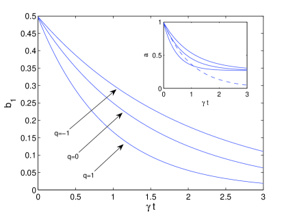
Figure 1 shows the decay of the coherence ($b_{1}(t)$) for a qubit in a quon environment at temperature $T/\Omega=1$, for different values of the deformation parameter. From Eq.s (35), (36), (38), it follows that the decay of coherence at $q=-1$, and any finite temperature, behaves as the decay at $T=0$ and any $q$. In the inset, it is shown the decay of the population $a(t)$ (solid lines refer again to $T/\Omega=1$, while dashed line refers $T=0$). Thus, the fermionic environment gives rise to the slowest decay of coherence and population. The decay of quantum coherence becomes slower and slower when passing from the bosonic to fermionic environment.

Refer to caption
Figure 1: The plot shows the decay of the coherence $b_{1}(t)$ for a qubit in a quon-environment at temperature $T/\Omega=1$, for different values of the deformation parameter. In the inset, it is shown the decay of the population $a(t)$ (solid lines refer again to $T/\Omega=1$, dashed line refers $T=0$).

V Two qubits in the same environment

We now assume the system composed by two identical qubits interacting with the same environment. Then the master equation can be written as Eq.(III) simply replacing $\sigma$ with $\sigma_{1}+\sigma_{2}$, that is

$\displaystyle\dot{\rho}(t)$ $\displaystyle=$ $\displaystyle-\frac{\gamma}{2}\langle[N]_{q}\rangle_{E}\left(\sigma_{1}\sigma_{1}^{{\dagger}}\rho(t)-2\sigma_{1}^{{\dagger}}\rho(t)\sigma_{1}+\rho(t)\sigma_{1}\sigma_{1}^{{\dagger}}+\sigma_{2}\sigma_{2}^{{\dagger}}\rho(t)\right.$ (40)
βˆ’2​σ2†​ρ​(t)​σ2+ρ​(t)​σ2​σ2†+Οƒ1​σ2†​ρ​(t)+Οƒ2​σ1†​ρ​(t)2superscriptsubscript𝜎2β€ πœŒπ‘‘subscript𝜎2πœŒπ‘‘subscript𝜎2superscriptsubscript𝜎2†subscript𝜎1superscriptsubscript𝜎2β€ πœŒπ‘‘subscript𝜎2superscriptsubscript𝜎1β€ πœŒπ‘‘\displaystyle\qquad\qquad\quad-2\sigma_{2}^{{\dagger}}\rho(t)\sigma_{2}+\rho(t)\sigma_{2}\sigma_{2}^{{\dagger}}+\sigma_{1}\sigma_{2}^{{\dagger}}\rho(t)+\sigma_{2}\sigma_{1}^{{\dagger}}\rho(t)
$\displaystyle\qquad\qquad\quad\left.-2\sigma_{1}^{{\dagger}}\rho(t)\sigma_{2}-2\sigma_{2}^{{\dagger}}\rho(t)\sigma_{1}+\rho(t)\sigma_{1}\sigma_{2}^{{\dagger}}+\rho(t)\sigma_{2}\sigma_{1}^{{\dagger}}\right)$
$\displaystyle-$ $\displaystyle\frac{\gamma}{2}\langle[N+1]_{q}\rangle_{E}\left(\sigma_{1}^{{\dagger}}\sigma_{1}\rho(t)-2\sigma_{1}\rho(t)\sigma_{1}^{{\dagger}}+\rho(t)\sigma_{1}^{{\dagger}}\sigma_{1}+\sigma_{2}^{{\dagger}}\sigma_{2}\rho(t)\right.$
βˆ’2​σ2​ρ​(t)​σ2†+ρ​(t)​σ2†​σ2+Οƒ1†​σ2​ρ​(t)+Οƒ2†​σ1​ρ​(t)2subscript𝜎2πœŒπ‘‘superscriptsubscript𝜎2β€ πœŒπ‘‘superscriptsubscript𝜎2†subscript𝜎2superscriptsubscript𝜎1†subscript𝜎2πœŒπ‘‘superscriptsubscript𝜎2†subscript𝜎1πœŒπ‘‘\displaystyle\qquad\qquad\quad-2\sigma_{2}\rho(t)\sigma_{2}^{{\dagger}}+\rho(t)\sigma_{2}^{{\dagger}}\sigma_{2}+\sigma_{1}^{{\dagger}}\sigma_{2}\rho(t)+\sigma_{2}^{{\dagger}}\sigma_{1}\rho(t)
βˆ’2Οƒ1ρ(t)Οƒ2β€ βˆ’2Οƒ2ρ(t)Οƒ1†+ρ(t)Οƒ1†σ2+ρ(t)Οƒ2†σ1).\displaystyle\qquad\qquad\quad\left.-2\sigma_{1}\rho(t)\sigma_{2}^{{\dagger}}-2\sigma_{2}\rho(t)\sigma_{1}^{{\dagger}}+\rho(t)\sigma_{1}^{{\dagger}}\sigma_{2}+\rho(t)\sigma_{2}^{{\dagger}}\sigma_{1}\right).

Then, we proceed in the same way as for the single qubit case. That is, we consider the operators appearing in Eq.(40) and represent them in matrix form in the computational basis $\{|00\rangle,|01\rangle|10\rangle,|11\rangle\}$,

$\displaystyle\sigma_{1}=\left(\begin{array}[]{cccc}0&0&0&0\\ 0&0&0&0\\ 1&0&0&0\\ 0&1&0&0\end{array}\right),\quad\sigma_{2}=\left(\begin{array}[]{cccc}0&0&0&0\\ 1&0&0&0\\ 0&0&0&0\\ 0&0&1&0\end{array}\right),$ (49)

and

$\displaystyle\rho(t)=\left(\begin{array}[]{cccc}a(t)&b_{1}(t)+\iota b_{2}(t)&c_{1}(t)+\iota c_{2}(t)&d_{1}(t)+\iota d_{2}(t)\\ b_{1}(t)-\iota b_{2}(t)&e(t)&f_{1}(t)+\iota f_{2}(t)&g_{1}(t)+\iota g_{2}(t)\\ c_{1}(t)-\iota c_{2}(t)&f_{1}(t)-\iota f_{2}(t)&h(t)&i_{1}(t)+\iota i_{2}(t)\\ d_{1}(t)-\iota d_{2}(t)&g_{1}(t)-\iota g_{2}(t)&i_{1}(t)-\iota i_{2}(t)&1-a(t)-e(t)-h(t)\end{array}\right),$ (54)

where $a(t)$, $b_{1}(t)$, $b_{2}(t)$, $c_{1}(t)$, $c_{2}(t)$, $d_{1}(t)$, $d_{2}(t)$, $e(t)$, $f_{1}(t)$, $f_{2}(t)$, $g_{1}(t)$, $g_{2}(t)$, $h(t)$, $i_{1}(t)$ and $i_{2}(t)$ are real functions of time to be determined. In terms of these functions, the master equation is written as a set of coupled differential equations. They are reported together with their solutions in Appendix A.

In this case, a relevant quantity to study is the entanglement between the two qubits. Specifically we consider the qubits initialized in one of the four Bell states

$\displaystyle|\phi_{\pm}\rangle$ $\displaystyle=$ $\displaystyle 2^{-1/2}(|00\rangle\pm|11\rangle),$ (55)
$\displaystyle|\psi_{\pm}\rangle$ $\displaystyle=$ $\displaystyle 2^{-1/2}(|01\rangle\pm|10\rangle),$ (56)

and then we investigate how entanglement decays.

We use the concurrence as measure of the degree of entanglement Woot

$$C(\rho(t))=\max\left\{0,\lambda_{1}(t)-\lambda_{2}(t)-\lambda_{3}(t)-\lambda_{4}(t)\right\},$$ (57)

where $\lambda_{i}(t)$’s are, in decreasing order, the nonnegative square roots of the moduli of the eigenvalues of $\rho(t)\tilde{\rho}(t)$ with

$$\tilde{\rho}(t)=\left(\sigma_{1}-\sigma_{1}^{{\dagger}}\right)\left(\sigma_{2}-\sigma_{2}^{{\dagger}}\right)\rho^{*}(t)\left(\sigma_{1}-\sigma_{1}^{{\dagger}}\right)\left(\sigma_{2}-\sigma_{2}^{{\dagger}}\right),$$ (58)

and $\rho^{*}(t)$ denotes the complex conjugate of $\rho(t)$.

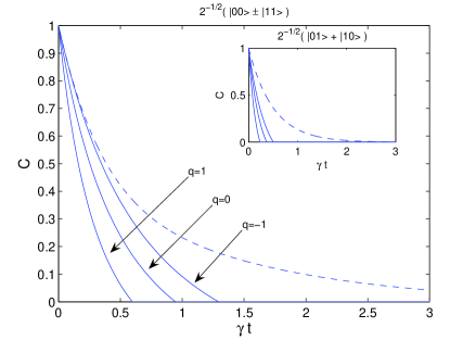
The decay of the concurrence is plotted in Figure 2. The qubits are initialized in the Bell states (55). For $T/\Omega=0$, the decay of the concurrence is independent from the deformation parameter $q$. For $T/\Omega>0$ we see the phenomenon of entanglement sudden death ESD . We notice however that the entanglement death time depends on the value of the deformation parameter $q$. In particular, the slowest decay and the longest lifetime of entanglement is evident for the fermionic case $q=-1$. The same happens when the two-qubit state is initialized in $|\psi_{+}\rangle=2^{-1/2}(|01\rangle+|10\rangle)$ (see inset). The decay of concurrence is slower and slower when continuously passing from the bosonic to the fermionic environment. On the contrary, the Bell state $|\psi_{-}\rangle$ is invariant under the dynamics of (40), thus entanglement in this case is totally preserved.

Refer to caption
Figure 2: The plot shows the decay of the concurrence for the two-qubit system in a quon-environment. Both qubits are plunged into the same environment. The qubits are initialized in one of the Bell states $|\phi_{\pm}\rangle=2^{-1/2}(|00\rangle\pm|11\rangle)$; dashed line refer to $T/\Omega=0$, solid lines to $T/\Omega=1$ and several values of the deformation parameter $q$. In the inset the two-qubit state is initialized in the Bell state $|\psi_{+}\rangle=2^{-1/2}(|01\rangle+|10\rangle)$. The remaining Bell state $|\psi_{-}\rangle=2^{-1/2}(|01\rangle-|10\rangle)$ is preserved by the dynamics.

VI Two qubits in separate environments

Here we consider each of the two identical qubit interacting with its own environment. Then the master equation is a straightforward extension of Eq.(III), that is

$\displaystyle\dot{\rho}(t)$ $\displaystyle=$ βˆ’Ξ³2β€‹βŸ¨[N]q⟩E​(Οƒ1​σ1†​ρ​(t)βˆ’2​σ1†​ρ​(t)​σ1+ρ​(t)​σ1​σ1†+Οƒ2​σ2†​ρ​(t)βˆ’2​σ2†​ρ​(t)​σ2+ρ​(t)​σ2​σ2†)𝛾2subscriptdelimited-⟨⟩subscriptdelimited-[]π‘π‘žπΈsubscript𝜎1superscriptsubscript𝜎1β€ πœŒπ‘‘2superscriptsubscript𝜎1β€ πœŒπ‘‘subscript𝜎1πœŒπ‘‘subscript𝜎1superscriptsubscript𝜎1†subscript𝜎2superscriptsubscript𝜎2β€ πœŒπ‘‘2superscriptsubscript𝜎2β€ πœŒπ‘‘subscript𝜎2πœŒπ‘‘subscript𝜎2superscriptsubscript𝜎2†\displaystyle-\frac{\gamma}{2}\langle[N]_{q}\rangle_{E}\left(\sigma_{1}\sigma_{1}^{{\dagger}}\rho(t)-2\sigma_{1}^{{\dagger}}\rho(t)\sigma_{1}+\rho(t)\sigma_{1}\sigma_{1}^{{\dagger}}+\sigma_{2}\sigma_{2}^{{\dagger}}\rho(t)-2\sigma_{2}^{{\dagger}}\rho(t)\sigma_{2}+\rho(t)\sigma_{2}\sigma_{2}^{{\dagger}}\right) (59)
βˆ’Ξ³2β€‹βŸ¨[N+1]q⟩E​(Οƒ1†​σ1​ρ​(t)βˆ’2​σ1​ρ​(t)​σ1†+ρ​(t)​σ1†​σ1+Οƒ2†​σ2​ρ​(t)βˆ’2​σ2​ρ​(t)​σ2†+ρ​(t)​σ2†​σ2).𝛾2subscriptdelimited-⟨⟩subscriptdelimited-[]𝑁1π‘žπΈsuperscriptsubscript𝜎1†subscript𝜎1πœŒπ‘‘2subscript𝜎1πœŒπ‘‘superscriptsubscript𝜎1β€ πœŒπ‘‘superscriptsubscript𝜎1†subscript𝜎1superscriptsubscript𝜎2†subscript𝜎2πœŒπ‘‘2subscript𝜎2πœŒπ‘‘superscriptsubscript𝜎2β€ πœŒπ‘‘superscriptsubscript𝜎2†subscript𝜎2\displaystyle-\frac{\gamma}{2}\langle[N+1]_{q}\rangle_{E}\left(\sigma_{1}^{{\dagger}}\sigma_{1}\rho(t)-2\sigma_{1}\rho(t)\sigma_{1}^{{\dagger}}+\rho(t)\sigma_{1}^{{\dagger}}\sigma_{1}+\sigma_{2}^{{\dagger}}\sigma_{2}\rho(t)-2\sigma_{2}\rho(t)\sigma_{2}^{{\dagger}}+\rho(t)\sigma_{2}^{{\dagger}}\sigma_{2}\right).

It can be solved with the same method of (40). The corresponding differential equations and their solutions are reported in Appendix B.

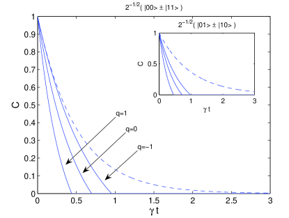
Figure 3 shows the decay of the concurrence in time. The qubits are initialized in the Bell states (55). For $T/\Omega=0$, the concurrence decay is independent from the deformation parameter $q$. Also in this case, for $T/\Omega>0$, we see the phenomenon of entanglement sudden death ESD . We notice that the entanglement death time depends on the value of the deformation parameter $q$. In particular, the slowest decay and the longest lifetime of entanglement is for the fermionic case $q=-1$. The same happens when the two-qubit state is initialized in $|\psi_{\pm}\rangle=2^{-1/2}(|01\rangle\pm|10\rangle)$ (see inset). The decay of entanglement becomes slower and slower when passing from the bosonic to the fermionic environment. In this case there is no maximally entangled state that remains invariant under the dynamics.

Refer to caption
Figure 3: The plot shows the decay of the concurrence of the two-qubit system in a quon-environment. Each qubit is subject to independent and identical environment. The qubits are initialized in one of the Bell states $|\phi_{\pm}\rangle=2^{-1/2}(|00\rangle\pm|11\rangle)$; dashed line refer to $T/\Omega=0$, solid lines to $T/\Omega=1$ and several values of the deformation parameter $q$. In the inset the two-qubit state is initialized in one of the Bell states $|\psi_{\pm}\rangle=2^{-1/2}(|01\rangle\pm|10\rangle)$.

VII Conclusion

In conclusion, we have analyzed the qubit dynamics in an environment of oscillators satisfying suitable $q$-deformed commutation relations, such that it permits to interpolate between oscillators and spin-$\frac{1}{2}$ particles. Specifically we have evaluated the decay of quantum coherence and entanglement in time when passing from bosonic to fermionic environments. The general behavior is that, at finite temperature, coherence and entanglement decay slower and slower when continuously passing from bosonic to fermionic environments.

Our work sheds further light on the mechanism of loosing quantum coherence and paves the way for a deeper algebraic analysis of this phenomenon. Moreover it could be useful for describing realistic physical situations where the assumption of an interaction with an environment of solely oscillators (resp. spin-$\frac{1}{2}$) particle turns out to be oversimplified.

Acknowledgements

The work of C.L. and S.M. is partially supported by EU through the FET-Open Project HIP (FP7-ICT-221899).

Appendix A Two qubits in the same environment

Using the parametrization in (54), the master equation (40) translates in the following set of differential equations

$\displaystyle\frac{d}{dt}a$ $\displaystyle=$ $\displaystyle-4Ba+2A(e+2f_{1}+h)$ (60)
$\displaystyle\frac{d}{dt}(b_{1}+\iota b_{2})$ $\displaystyle=$ $\displaystyle-B(3b_{1}+3\iota b_{2}+c_{1}+\iota c_{2})$ (61)
$\displaystyle-A(b_{1}+\iota b_{2}+c_{1}+\iota c_{2}-2g_{1}-2\iota g_{2}-2i_{1}-2\iota i_{2})$
$\displaystyle\frac{d}{dt}(c_{1}+\iota c_{2})$ $\displaystyle=$ $\displaystyle-B(b_{1}+\iota b_{2}+3c_{1}+3\iota c_{2})$ (62)
$\displaystyle-A(b_{1}+\iota b_{2}+c_{1}+\iota c_{2}-2g_{1}-2\iota g_{2}-2i_{1}-2\iota i_{2})$
$\displaystyle\frac{d}{dt}(d_{1}+\iota d_{2})$ $\displaystyle=$ $\displaystyle-2(A+B)(d_{1}+\iota d_{2})$ (63)
$\displaystyle\frac{d}{dt}e$ $\displaystyle=$ $\displaystyle 2B(a-e-f_{1})+A(a+2e+h+f_{1}-1)$ (64)
$\displaystyle\frac{d}{dt}(f_{1}+\iota f_{2})$ $\displaystyle=$ $\displaystyle B(2a-e-h-2f_{1}-2\iota f_{2})$ (65)
$\displaystyle+A(2-2a-3e-3h-2f_{1}-2\iota f_{2})$
$\displaystyle\frac{d}{dt}(g_{1}+\iota g_{2})$ $\displaystyle=$ $\displaystyle B(2b_{1}+2\iota b_{2}+2c_{1}+2\iota c_{2}-g_{1}-\iota g_{2}-i_{1}-\iota i_{2})$ (66)
$\displaystyle-A(3g_{1}+3\iota g_{2}+i_{1}+\iota i_{2})$
$\displaystyle\frac{d}{dt}h$ $\displaystyle=$ $\displaystyle 2B(a-h-f_{1})-2A(a+e+2h+f_{1}-1)$ (67)
$\displaystyle\frac{d}{dt}(i_{1}+\iota i_{2})$ $\displaystyle=$ $\displaystyle B(2b_{1}+2\iota b_{2}+2c_{1}+2\iota c_{2}-g_{1}-\iota g_{2}-i_{1}-\iota i_{2})$ (68)
$\displaystyle-A(g_{1}+\iota g_{2}+3i_{1}+3\iota i_{2})$

The solutions of the differential equations (60)-(68) read

$\displaystyle a(t)$ $\displaystyle=$ $\displaystyle\frac{1}{4\sqrt{B}}e^{-4(\sqrt{AB}+B)t}\left[2a(0)\sqrt{B}\left(1+e^{8\sqrt{AB}t}\right)\right.$ (69)
$\displaystyle\left.+\sqrt{A}\left(e^{8\sqrt{AB}t}-1\right)\left(e(0)+2f_{1}(0)+h(0)\right)\right],$
$\displaystyle b_{1}(t)$ $\displaystyle=$ $\displaystyle\frac{e^{-\left(3A+3B+\Theta\right)t}}{4\Theta^{2}}\left\{A^{2}\left[c_{1}(0)\left(1+e^{2\Theta t}-2e^{\left(3A+B+\Theta\right)t}\right)\right.\right.$ (70)
$\displaystyle\left.+b_{1}(0)\left(1+e^{2\Theta t}+2e^{\left(3A+B+\Theta\right)t}\right)\right]+B\Theta(b_{1}(0)+c_{1}(0))\left(1-e^{2\Theta t}\right)$
$\displaystyle+B^{2}\left[+c_{1}(0)\left(1+e^{2\Theta t}-2e^{\left(3A+B+\Theta\right)t}\right)+b_{1}(0)\left(1+e^{2\Theta t}+2e^{\left(3A+B+\Theta\right)t}\right)\right]$
$\displaystyle\left.+A\left[14B\left(c_{1}(0)\left(1+e^{2\Theta t}-2e^{\left(3A+B+\Theta\right)t}\right)+b_{1}(0)\left(1+e^{2\Theta t}+2e^{\left(3A+B+\Theta\right)t}\right)\right)\right.\right.$
$\displaystyle\left.\left.+\Theta\left(-1+e^{2\Theta t}\right)(b_{1}(0)+c_{1}(0)+4g_{1}(0)+4i_{1}(0))\right]\right\},$
$\displaystyle c_{1}(t)$ $\displaystyle=$ $\displaystyle\frac{e^{-\left(3A+3B+\Theta\right)t}}{4\Theta^{2}}\left\{A^{2}\left[b_{1}(0)\left(1+e^{2\Theta t}-2e^{\left(3A+B+\Theta\right)t}\right)\right.\right.$ (71)
$\displaystyle\left.+c_{1}(0)\left(1+e^{2\Theta t}+2e^{\left(3A+B+\Theta\right)t}\right)\right]+B\Theta(b_{1}(0)+c_{1}(0))\left(1-e^{2\Theta t}\right)$
$\displaystyle+B^{2}\left[b_{1}(0)\left(1+e^{2\Theta t}-2e^{\left(3A+B+\Theta\right)t}\right)+c_{1}(0)\left(1+e^{2\Theta t}+2e^{\left(3A+B+\Theta\right)t}\right)\right]$
$\displaystyle+A\left[14B\left(b_{1}(0)\left(1+e^{2\Theta t}-2e^{\left(3A+B+\Theta\right)t}\right)+c_{1}(0)\left(1+e^{2\Theta t}+2e^{\left(3A+B+\Theta\right)t}\right)\right)\right.$
$\displaystyle\left.\left.+\Theta\left(-1+e^{2\Theta t}\right)(b_{1}(0)+c_{1}(0)+4g_{1}(0)+4i_{1}(0))\right]\right\},$
$\displaystyle d_{1}(t)$ $\displaystyle=$ $\displaystyle d_{1}(0)e^{-2(A+B)t},$ (72)
$\displaystyle e(t)$ $\displaystyle=$ $\displaystyle\frac{e^{-2\left(3A+2\sqrt{AB}+3B\right)t}}{8\sqrt{AB}\left(A^{2}-3AB+B^{2}\right)}\left\{-2a(0)AB^{2}e^{2(3A+B)t}\left(e^{8\sqrt{AB}t}-1\right)\right.$ (73)
$\displaystyle+2a(0)B^{3}e^{2(3A+B)t}\left(e^{8\sqrt{AB}t}-1\right)$
$\displaystyle-A^{3}e^{2(3A+B)t}\left(e^{8\sqrt{AB}t}-1\right)(e(0)+2f_{1}(0)+h(0))$
$\displaystyle+3A^{2}Be^{2(3A+B)t}\left(e^{8\sqrt{AB}t}-1\right)(e(0)+2f_{1}(0)+h(0))$
$\displaystyle+\sqrt{AB^{5}}e^{2(A+B)t}\left[4e^{4\left(A+\sqrt{AB}+B\right)t}+4e^{2\left(\sqrt{A}+\sqrt{B}\right)^{2}t}(e(0)-h(0))\right.$
$\displaystyle+2e^{4\sqrt{AB}t+4Bt}(e(0)-2f_{1}(0)+h(0)-2)$
$\displaystyle\left.+e^{4At}(e(0)+2f_{1}(0)+h(0))+e^{4At+8\sqrt{AB}t}(e(0)+2f_{1}(0)+h(0))\right]$
$\displaystyle-\sqrt{A^{3}B^{3}}e^{2(A+B)t}\left[12e^{4\left(A+\sqrt{AB}+B\right)t}+12e^{2\left(\sqrt{A}+\sqrt{B}\right)^{2}t}(e(0)-h(0))\right.$
$\displaystyle\left.-6a(0)\left(e^{4At}+e^{4At+8\sqrt{AB}t}-2e^{4\sqrt{AB}t+4Bt}\right)+e^{4At}(e(0)+2f_{1}(0)+h(0))\right.$
$\displaystyle+e^{4At+8\sqrt{AB}t}(e(0)+2f_{1}(0)+h(0))$
$\displaystyle\left.+2e^{4\sqrt{AB}t+4Bt}(5e(0)-2f_{1}(0)+5h(0)-6)\right]$
$\displaystyle\left.+2\sqrt{A^{5}B}\left[-a(0)\left(e^{2(3A+B)t}+e^{2\left(3A+4\sqrt{AB}+B\right)t}-2e^{2\left(A+2\sqrt{AB}+3B\right)t}\right)\right.\right.$
$\displaystyle+2e^{2\left(A+2\sqrt{AB}+2B\right)t}\left(e^{2(2A+B)t}+e^{2At}(e(0)-h(0))\right.$
$\displaystyle\left.\left.\left.+e^{2Bt}(e(0)+h(0)-1)\right)\right]\right\},$
$\displaystyle f_{1}(t)$ $\displaystyle=$ $\displaystyle\frac{e^{-4\left(A+\sqrt{AB}+B\right)t}}{8\sqrt{AB}\left(A^{2}-3AB+B^{2}\right)}\left\{-10a(0)AB^{2}e^{4At}\left(e^{8\sqrt{AB}t}-1\right)\right.$ (74)
$\displaystyle+2a(0)B^{3}e^{4At}\left(e^{8\sqrt{AB}t}-1\right)+A^{3}e^{4At}\left(e^{8\sqrt{AB}t}-1\right)(e(0)+2f_{1}(0)+h(0))$
$\displaystyle+A^{2}Be^{4At}\left(e^{8\sqrt{AB}t}-1\right)(4a(0)-3e(0)-6f_{1}(0)-3h(0))$
$\displaystyle-2\sqrt{A^{5}B}\left[2e^{4\left(A+\sqrt{AB}+B\right)t}-a(0)\left(e^{4At}-2e^{4\left(\sqrt{AB}+B\right)t}+e^{4At+8\sqrt{AB}t}\right)\right.$
$\displaystyle+2e^{4\left(\sqrt{AB}+B\right)t}(e(0)+h(0)-1)$
$\displaystyle\left.\left.-e^{4At}(e(0)+2f_{1}(0)+h(0))-e^{4At+8\sqrt{AB}t}(e(0)+2f_{1}(0)+h(0))\right]\right.$
$\displaystyle+\sqrt{AB^{5}}\left[-4e^{4\left(A+\sqrt{AB}+B\right)t}-2e^{4\left(\sqrt{AB}+B\right)t}(e(0)-2f_{1}(0)+h(0)-2)\right.$
$\displaystyle\left.+e^{4At}(e(0)+2f_{1}(0)+h(0))+e^{4At+8\sqrt{AB}t}(e(0)+2f_{1}(0)+h(0))\right]$
$\displaystyle+\sqrt{A^{3}B^{3}}\left[12e^{4\left(A+\sqrt{AB}+B\right)t}-6a(0)\left(e^{4At}-2e^{4\left(\sqrt{AB}+B\right)t}+e^{4At+8\sqrt{AB}t}\right)\right.$
$\displaystyle-5e^{4At}(e(0)+2f_{1}(0)+h(0))-5e^{4At+8\sqrt{AB}t}(e(0)+2f_{1}(0)+h(0))$
$\displaystyle\left.\left.+2e^{4\left(\sqrt{AB}+B\right)t}(5e(0)-2f_{1}(0)+5h(0)-6)\right]\right\},$
$\displaystyle f_{2}(t)$ $\displaystyle=$ $\displaystyle f_{2}(0)e^{-2(A+B)t},$ (75)
$\displaystyle g_{1}(t)$ $\displaystyle=$ $\displaystyle\frac{e^{-\left(3A+3B+\Theta\right)t}}{4\Theta^{2}}\left\{B\left[4\Theta\left(b_{1}(0)+c_{1}(0)\right)\left(-1+e^{2\Theta t}\right)+14A\left(g_{1}(0)+i_{1}(0)\right)\right.\right.$
$\displaystyle-\Theta\left(g_{1}(0)+i_{1}(0)\right)+\Theta e^{2\Theta t}\left(g_{1}(0)+i_{1}(0)\right)$
$\displaystyle\left.+28Ae^{\left(A+3B+\Theta\right)t}\left(g_{1}(0)-i_{1}(0)\right)+14Ae^{2\Theta t}\left(g_{1}(0)+i_{1}(0)\right)\right]$
$\displaystyle+B^{2}\left[\left(1+e^{2\Theta t}+2e^{\left(A+3B+\Theta\right)t}\right)g_{1}(0)+\left(1+e^{2\Theta t}-2e^{\left(A+3B+\Theta\right)t}\right)i_{1}(0)\right]$
$\displaystyle+A\left[\Theta\left(1-e^{2\Theta t}\right)(g_{1}(0)+i_{1}(0))+A\left(\left(1+e^{2\Theta t}+2e^{\left(A+3B+\Theta\right)t}\right)g_{1}(0)\right.\right.$
$\displaystyle+\left.\left.\left.\left(1+e^{2\Theta t}-2e^{\left(A+3B+\Theta\right)t}\right)i_{1}(0)\right)\right]\right\},$
$\displaystyle h(t)$ $\displaystyle=$ $\displaystyle\frac{e^{-2\left(3A+2\sqrt{AB}+3B\right)t}}{8\sqrt{AB}\left(A^{2}-3AB+B^{2}\right)}\left\{-2a(0)AB^{2}e^{2(3A+B)t}\left(e^{8\sqrt{AB}t}-1\right)\right.$ (77)
$\displaystyle+2a(0)B^{3}e^{2(3A+B)t}\left(e^{8\sqrt{AB}t}-1\right)$
$\displaystyle-A^{3}e^{2(3A+B)t}\left(e^{8\sqrt{AB}t}-1\right)(e(0)+2f_{1}(0)+h(0))$
$\displaystyle+3A^{2}Be^{2(3A+B)t}\left(e^{8\sqrt{AB}t}-1\right)(e(0)+2f_{1}(0)+h(0))$
$\displaystyle+\sqrt{AB^{5}}e^{2(A+B)t}\left[4e^{4\left(A+\sqrt{AB}+B\right)t}-4e^{2\left(\sqrt{A}+\sqrt{B}\right)^{2}t}(e(0)-h(0))\right.$
$\displaystyle+2e^{4\sqrt{AB}t+4Bt}(e(0)-2f_{1}(0)+h(0)-2)$
$\displaystyle\left.\left.+e^{4At}(e(0)+2f_{1}(0)+h(0))+e^{4At+8\sqrt{AB}t}(e(0)+2f_{1}(0)+h(0))\right]\right.$
$\displaystyle-\sqrt{A^{3}B^{3}}e^{2(A+B)t}\left[12e^{4\left(A+\sqrt{AB}+B\right)t}\right.$
$\displaystyle-6a(0)\left(e^{4At}+e^{4At+8\sqrt{AB}t}-2e^{4\sqrt{AB}t+4Bt}\right)$
$\displaystyle-12e^{2\left(\sqrt{A}+\sqrt{B}\right)^{2}t}(e(0)-h(0))+e^{4At}(e(0)+2f_{1}(0)+h(0))$
$\displaystyle+e^{4At+8\sqrt{AB}t}(e(0)+2f_{1}(0)+h(0))$
$\displaystyle\left.+2e^{4\sqrt{AB}t+4Bt}(5e(0)-2f_{1}(0)+5h(0)-6)\right]$
$\displaystyle\left.+2\sqrt{A^{5}B}\left[-a(0)\left(e^{2(3A+B)t}+e^{2\left(3A+4\sqrt{AB}+B\right)t}-2e^{2\left(A+2\sqrt{AB}+3B\right)t}\right)\right.\right.$
$\displaystyle+2e^{2\left(A+2\sqrt{AB}+2B\right)t}\left(e^{2(2A+B)t}-e^{2At}(e(0)-h(0))\right.$
$\displaystyle\left.\left.\left.+e^{2Bt}(e(0)+h(0)-1)\right)\right]\right\},$
$\displaystyle i_{1}(t)$ $\displaystyle=$ $\displaystyle\frac{e^{-\left(3A+3B+\Theta\right)t}}{4\Theta^{2}}\left\{B\left[4\Theta\left(b_{1}(0)+c_{1}(0)\right)\left(-1+e^{2\Theta t}\right)\right.\right.$ (78)
$\displaystyle+14A\left(g_{1}(0)+i_{1}(0)\right)-\Theta\left(g_{1}(0)+i_{1}(0)\right)+\Theta e^{2\Theta t}\left(g_{1}(0)+i_{1}(0)\right)$
$\displaystyle\left.\left.-28Ae^{\left(A+3B+\Theta\right)t}\left(g_{1}(0)-i_{1}(0)\right)+14Ae^{2\Theta t}\left(g_{1}(0)+i_{1}(0)\right)\right]\right.$
$\displaystyle\left.+B^{2}\left[\left(1+e^{2\Theta t}-2e^{\left(A+3B+\Theta\right)t}\right)g_{1}(0)+\left(1+e^{2\Theta t}+2e^{\left(A+3B+\Theta\right)t}\right)i_{1}(0)\right]\right.$
$\displaystyle+A^{2}\left[\left(1+e^{2\Theta t}-2e^{\left(A+3B+\Theta\right)t}\right)g_{1}(0)+\left(1+e^{2\Theta t}+2e^{\left(A+3B+\Theta\right)t}\right)i_{1}(0)\right]$
$\displaystyle\left.+A\left[\Theta\left(1-e^{2\Theta t}\right)(g_{1}(0)+i_{1}(0))\right]\right\},$

where $\Theta=\sqrt{A^{2}+14AB+B^{2}}$. The other solutions $b_{2}(t)$, $c_{2}(t)$, $d_{2}(t)$, $g_{2}(t)$ and $i_{2}(t)$ can be obtained from $b_{1}(t)$, $c_{1}(t)$, $d_{1}(t)$, $g_{1}(t)$ and $i_{1}(t)$ respectively by simply replacing the subscripts $1\to 2$.

Appendix B Two qubits in separate environments

Using the parametrization in (54), the master equation (59) translates in the following set of differential equations

$\displaystyle\frac{d}{dt}a$ $\displaystyle=$ $\displaystyle-4Ba+2A(e+h),$ (79)
$\displaystyle\frac{d}{dt}(b_{1}+\iota b_{2})$ $\displaystyle=$ $\displaystyle-3B(b_{1}+\iota b_{2})-A(b_{1}+\iota b_{2}-2i_{1}-2\iota i_{2}),$ (80)
$\displaystyle\frac{d}{dt}(c_{1}+\iota c_{2})$ $\displaystyle=$ $\displaystyle-3B(c_{1}+\iota c_{2})-A(c_{1}+\iota c_{2}-2g_{1}-2\iota g_{2}),$ (81)
$\displaystyle\frac{d}{dt}(d_{1}+\iota d_{2})$ $\displaystyle=$ $\displaystyle-2(A+B)(d_{1}+\iota d_{2}),$ (82)
$\displaystyle\frac{d}{dt}e$ $\displaystyle=$ $\displaystyle 2B(a-e)-2A(a+2e+h-1),$ (83)
$\displaystyle\frac{d}{dt}(f_{1}+\iota f_{2})$ $\displaystyle=$ $\displaystyle-2(A+B)(f_{1}+\iota f_{2}),$ (84)
$\displaystyle\frac{d}{dt}(g_{1}+\iota g_{2})$ $\displaystyle=$ $\displaystyle B(2c_{1}+2\iota c_{2}-g_{1}-\iota g_{2})-3A(g_{1}+\iota g_{2}),$ (85)
$\displaystyle\frac{d}{dt}h$ $\displaystyle=$ $\displaystyle 2B(a-h)-2A(a+e+2h-1),$ (86)
$\displaystyle\frac{d}{dt}(i_{1}+\iota i_{2})$ $\displaystyle=$ $\displaystyle B(2b_{1}+2\iota b_{2}-i_{1}-\iota i_{2})-3A(i_{1}+\iota i_{2}).$ (87)

The solutions of the differential equations (79)-(87) read

$\displaystyle a(t)$ $\displaystyle=$ $\displaystyle\frac{e^{-4(A+B)t}}{(A+B)^{2}}\left\{a(0)B^{2}+A^{2}\left[a(0)\left(2e^{2(A+B)t}-1\right)\right.\right.$ (88)
$\displaystyle\qquad\qquad\quad\left.+\left(e^{2(A+B)t}-1\right)\left(e^{2(A+B)t}+e(0)+h(0)-1\right)\right]$
$\displaystyle\qquad\qquad\quad\left.+\left[2a(0)e^{2(A+B)t}+\left(e(0)+h(0)\right)\left(e^{2(A+B)t}-1\right)\right]AB\right\},$
$\displaystyle b_{1}(t)$ $\displaystyle=$ $\displaystyle\frac{e^{-3(A+B)t}}{A+B}\left\{b_{1}(0)B+A\left[b_{1}(0)e^{2(A+B)t}+\left(e^{2(A+B)t}-1\right)i_{1}(0)\right]\right\},$ (89)
$\displaystyle c_{1}(t)$ $\displaystyle=$ $\displaystyle\frac{e^{-3(A+B)t}}{A+B}\left\{c_{1}(0)B+A\left[c_{1}(0)e^{2(A+B)t}+\left(e^{2(A+B)t}-1\right)g_{1}(0)\right]\right\},$ (90)
$\displaystyle d_{1}(t)$ $\displaystyle=$ $\displaystyle d_{1}(0)e^{-2(A+B)t},$ (91)
$\displaystyle e(t)$ $\displaystyle=$ $\displaystyle\frac{e^{-4(A+B)t}}{(A+B)^{2}}\left\{\left[a(0)\left(1-e^{2(A+B)t}\right)+e(0)-e^{2(A+B)t}\left(h(0)-1\right)+h(0)-1\right]A^{2}\right.$ (92)
$\displaystyle\left.\qquad\qquad\quad+\left[e(0)+e^{4(A+B)t}+e^{2(A+B)t}\left(e(0)-h(0)-1\right)+h(0)\right]AB\right.$
$\displaystyle\left.\qquad\qquad\quad+\left[a(0)\left(e^{2(A+B)t}-1\right)+e(0)e^{2(A+B)t}\right]B^{2}\right\},$
$\displaystyle f_{1}(t)$ $\displaystyle=$ $\displaystyle f_{1}(0)e^{-2(A+B)t},$ (93)
$\displaystyle g_{1}(t)$ $\displaystyle=$ $\displaystyle\frac{e^{-3(A+B)t}}{A+B}\left\{g_{1}(0)B+A\left[g_{1}(0)e^{2(A+B)t}+\left(e^{2(A+B)t}-1\right)c_{1}(0)\right]\right\},$ (94)
$\displaystyle h(t)$ $\displaystyle=$ $\displaystyle\frac{e^{-4(A+B)t}}{(A+B)^{2}}\left\{\left[a(0)\left(1-e^{2(A+B)t}\right)-e^{2(A+B)t}\left(e(0)-1\right)+e(0)+h(0)-1\right]A^{2}\right.$ (95)
$\displaystyle\left.\qquad\qquad\quad+\left[e(0)+e^{4(A+B)t}+h(0)+e^{2(A+B)t}\left(h(0)-e(0)-1\right)\right]AB\right.$
$\displaystyle\left.\qquad\qquad\quad+\left[a(0)\left(e^{2(A+B)t}-1\right)+h(0)e^{2(A+B)t}\right]B^{2}\right\},$
$\displaystyle i_{1}(t)$ $\displaystyle=$ $\displaystyle\frac{e^{-3(A+B)t}}{A+B}\left\{i_{1}(0)B+A\left[i_{1}(0)e^{2(A+B)t}+\left(e^{2(A+B)t}-1\right)b_{1}(0)\right]\right\}.$ (96)

The other solutions $b_{2}(t)$, $c_{2}(t)$, $d_{2}(t)$, $f_{2}(t)$, $g_{2}(t)$ and $i_{2}(t)$ can be obtained from $b_{1}(t)$, $c_{1}(t)$, $d_{1}(t)$, $f_{1}(t)$, $g_{1}(t)$ and $i_{1}(t)$ respectively by simply replacing the subscripts $1\to 2$.

References

  • (1) C. W. Gardiner, Quantum Noise, Springer, Berlin 1991.
  • (2) V. Kuryshkin, Annales de la Fondation Louis de-Broglie 5 (1980), 111.
  • (3) P. Kulish and E. Damaskinsky, J.Β Phys.Β A 23 (1990), L415.
  • (4) A. J. Macfarlane, J.Β Phys.Β A 22 (1989), 4581;
    L. C. Biedenharn, J.Β Phys.Β A 22 (1989), L873;
    C.-P. Sun and H. C. Fu, J.Β Phys.Β A 22 (1989), L983.
  • (5) O. W. Greenberg, Phys.Β Rev.Β Lett.Β 64 (1990), 705; Phys.Β Rev.Β D 43 (1991), 4111.
  • (6) R. N. Mohapatra, Phys.Β Lett.Β B 242 (1990), 407.
  • (7) M. Chaichian et al., J.Β Phys.Β A 26 (1993), 4017.
  • (8) J. W. Goodison and D. J. Toms arXiv:hep-th/9410096.
  • (9) W. K. Wootters, Phys.Β Rev.Β Lett.Β 80 (1998), 2245.
  • (10) T. Yu and J. H. Eberly, Phys.Β Rev.Β Lett.Β 93 (2004), 140404;
    A. Al-Qasimi and D. F. V. James, Phys.Β Rev.Β A 77 (2008), 012117.