Time scales in nuclear giant resonances

Abstract

We propose a general approach to characterise fluctuations of measured cross sections of nuclear giant resonances. Simulated cross sections are obtained from a particular, yet representative self-energy which contains all information about fragmentations. Using a wavelet analysis, we demonstrate the extraction of time scales of cascading decays into configurations of different complexity of the resonance. We argue that the spreading widths of collective excitations in nuclei are determined by the number of fragmentations as seen in the power spectrum. An analytic treatment of the wavelet analysis using a Fourier expansion of the cross section confirms this principle. A simple rule for the relative life times of states associated with hierarchies of different complexity is given.

Nuclear Giant Resonances (GR) have been the subject of numerous investigations over several decades dstadta . Some of the basic features such as centroids and collectivity (in terms of the sum rules) are reasonably well understood within microscopic models BM2 ; micro . However, the question how a collective mode like the GR disseminates its energy is one of the central issues in nuclear structure physics.

According to accepted wisdom, GRs are essentially excited by an external field being a one-body interaction. It is natural to describe these states as collective 1p-1h states. Once excited, the GR disseminates its energy via direct particle emission and by coupling to more complicated configurations (2p-2h, 3p-3h, etc). The former mechanism gives rise to an escape width, while the latter yields spreading widths ($\Gamma^{\downarrow}$). An understanding of lifetime characteristics associated with the cascade of couplings and scales of fragmentations arising from this coupling (cf zel ; sok ; aiba ; lar ) remains a challenge. A recent high-resolution experiment of the Isoscalar Giant Quadrupole Resonance (QR) dstadtc ; dstadtd ; dstadte provides new insight for this problem.

It has been shown by Shevchenko et al. dstadtc that the fine structure of the QR observed in $(p,p^{\prime})$ experiments is largely probe independent. Furthermore, a study of the fine structure using wavelet analysis w1 ; w2 ; w3 reveals energy scales dstadtd ; dstadte in the widths of the fine structure displaying a seemingly schematic pattern, as can be seen in Fig.2. This pattern varies with the structure of the nucleus being studied. While the physical meaning of the results of such an analysis is still being debated, we try here to offer a general explanation. However, we do not embark on a specific microscopic analysis, but rather make use of general and well-established techniques of many-body theory. Gross effects due to nuclear deformation and coupling to the continuum sok are not discussed; we rather focus on the decay of the QR into configurations of various complexity.

To proceed we use the Green’s function approach. A central role is played by the self-energy whose finer structure is imparted upon the Green’s function via the solution of Dyson’s equation which reads mbody

$$G_{\alpha,\beta}(\omega)=((G^{0}_{\alpha,\beta}(\omega))^{-1}-\Sigma_{\alpha,\beta}(\omega))^{-1}$$ (1)

where we assume $G^{0}(\omega)={\delta_{\alpha,\beta}}/{(\omega-\epsilon)}$ to be diagonal in the basis $\alpha,\beta,\ldots$ while the complicated pole structure of $G(\omega)$ is generated by that of the self-energy $\Sigma_{\alpha,\beta}(\omega)$. The pole structure of $G$ carries over to the scattering matrix given by

$$T_{\alpha,\beta}(\omega)=\Sigma_{\alpha,\beta}(\omega)+\Sigma_{\alpha,\beta^{\prime}}(\omega)G_{\beta^{\prime},\alpha^{\prime}}(\omega)\Sigma_{\alpha^{\prime},\beta}(\omega)$$ (2)

from which a cross section $\sim|T_{\alpha,\alpha}(\omega)|^{2}$ is obtained.

Within the excitation energy range of the QR the nucleus has a high density of complicated states of several tens of thousands per MeV and even more for heavy nuclei. These many states appear in the self-energy as poles in the complex energy plane close to the real axis. The small widths imply they are long-lived states and traditionally classed as compound states. The simpler intermediate structure of the excitation is expressed by the substantial fluctuations of the corresponding residues associated with the poles of the self-energy $\Sigma(\omega)$ hahe . In other words, while the individual pole positions of $\Sigma(\omega)$ are virtually unstructured random , it is the variation of the corresponding residues that bears all the information about intermediate structure. Note that our approach differs from a traditional microscopic calculation in that we start from the outset from a random distribution of pole terms representing compound states. Traditional microscopic approaches cannot do justice to such structure ves and usually suffer from necessary truncation of configuration space and, associated with it, from possible inconsistencies and spurious states.

We assume that the QR being a collective 1p-1h state decays via a cascade progressing through (2p-2h)-, (3p-3h)-configurations and so forth to the eventual compound states. In turn, each of the intermediate states (including the initial QR) can either decay directly to the ground state or via some more complicated intermediate state. Below we will show that it is this mixture that is seen in the cross section and extracted by wavelet analysis, and it is the variety and cascading complexity of states that invokes the structure of the residues of the poles of the self-energy. Of importance to note is that the number of states available within the energy domain of the QR increases with its complexity: for example, six (2p-2h)-states, eleven (3p-3h)-states, down to several thousand compound states (the numbers six or eleven should be taken as examples without claim for quantitative correctness). Moreover, the corresponding life times are expected to increase in line with their increasing complexity, which is in accordance with their decreasing spreading widths (below we come back to this particular aspect of scaling).

Figure 1: Residues of the self-energy: for 6 (top) and 11 (bottom) intermediate states. The randomisation is clearly discernible.

As a typical case study we investigate here a wavelet analysis of a simulated cross section that results from a particular input for the self-energy. Since arbitrary units are used, we concentrate on the energy interval [0,1] and use for the pole position $\epsilon=0.5-i0.5$ of the single pole of $G_{0}$ (1). The number of compound states is assumed to be 300; this is of course much less than the experimental level density in the region of a QR for a medium or heavy nucleus, but it suffices for our demonstration. The real parts of the pole positions are assumed to be randomly distributed with a uniform distribution of the mean distance 1/300; the imaginary parts are randomly distributed in the interval [0.004,0.007].

For the sake of illustration we consider four sets of residues

$$r_{k}=\sum_{i=1}^{4}h_{i,k},\quad h_{i,k}=s\sum_{j=1}^{f_{i}}\frac{\gamma_{i}^{2}}{(\frac{k}{300}-j\cdot p_{i})^{2}+\gamma_{i}^{2}}$$ (3)

with an overall strength $s=10^{-5}$. This order of magnitude is based on the mean value of the widths of the compound states being about $10^{-4}$ to $10^{-5}$ times smaller than the $\Gamma^{\downarrow}\;(\gamma_{i})$. With these residues the self-energy reads

$$\Sigma(\omega)=\sum_{k=1}^{300}\frac{r_{k}}{\omega-\omega_{k}}$$ (4)

The poles at the complex positions $\omega_{k}$ occur in the lower $\omega$-plane with $\omega$ being the energy variable; the other symbols are explained in the text. If only $i=1$ was to occur with $f_{1}=6$, a typical pattern of the residues $r_{k}=h_{1,k}$ would be illustrated by the top of Fig.1; similarly for $f_{2}=11$ by the bottom. The inclusion of further terms would simply add additional peaks to the pattern. In the case presented below we have chosen $f_{2}=11,f_{3}=17$ and $f_{4}=29$ totalling to 6+11+17+29 additional peaks (not easily visualised, but beautifully discernible in the final analysis). We stress again that the four values $f_{i}$ were chosen for demonstration, more than four or other values can be used just as well.

These arbitrary numbers used in the example chosen describe particular fragmentations of the QR into altogether 6,11,17 and 29 states of increasing complexity. The widths $\gamma_{i}$ giving rise to the Lorentzian shape of the residues are in reality determined by the product of the density of the compound states and the coupling of the $i$-th group to the compound states. The widths are the spreading widths of the respective states considered hahe . As the complexity increases with label $i$ we shall assume $\gamma_{1}>\gamma_{2}>\gamma_{3}>\gamma_{4}$. In the simulation we endow each $\gamma_{i}$ with a random fluctuation with mean value $\gamma_{i}/4$. As stated above we refrain from specifying a microscopic structure causing the residue pattern assumed for the self-energy; below it becomes clear that guidance comes from experiment.

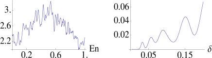
Figure 2: Simulated cross section (left) and power spectrum (right). Units are arbitrary. The abscissa of the cross section is the unit energy interval, the energy values $\delta$ on the abscissa of the power spectrum refer to the wavelet parameter using the same energy units.

We also assume that each set ${f_{i}}$ uniformly distributed over the whole energy interval. This is similar in spirit to the assumption used in the local scaling dimension approach aiba . The positions $p_{i}$ in Eq.(3) are set to be $\sim 1/f_{i}$ which spreads the actual $j\cdot p_{i}$ positions equidistantly over the whole interval with $j$ running from 1 to $f_{i}$; however, we endow them with a small random fluctuation with mean value $p_{i}/8$. Note that the random fluctuation of widths and positions generate a mild degree of asymmetry in the energy interval [0,1], resulting in slightly different patterns in the intervals [0,0.5] and [0.5,1]. The near equality of the positions, that is - apart from slight random fluctuations - the regular pattern of the various fragments as illustrated in Fig.1, is basically dictated by experimental findings: if there is no near regular pattern there will be no discernible structure in the power spectrum of the wavelet analysis. However, we shall return below to the case where such regular pattern may occur only in a smaller portion of the interval.

The first obvious choice for the widths assumes simply $\gamma_{i}=1/(2f_{i})$ yielding the simulated cross section shown in Fig.2 (below a precise analytic expression confirming the $1/(2f_{i})$-law is given). A variation of such choice is rather significant, we shall return to this aspect in detail.

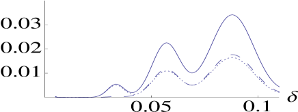
Figure 3: Power spectrum for a particular asymmetric situation discussed in text. The dotted curve originates from a scan of the interval [0,0.5], the dashed curve from [0.5,1] and the solid curve from the total interval. Note that the most left peak is virtually absent in the dashed curve while fully present in the dotted curve. Units as in Fig.2.

The analysis using a Morlet-type mother wavelet (a contour plot of the wavelet analysis is illustrated in Fig.5)

$$\frac{1}{\sqrt{\delta}}\,\cos\frac{k(\omega-\omega_{0})}{\delta}\,\exp-\frac{(\omega-\omega_{0})^{2}}{\delta^{2}}$$ (5)

gives the power spectrum shown in Fig.2; if not indicated otherwise we use the value $k=6$ for the wave number of the mother wavelet. There is in fact a $k$-dependence of the positions of the maxima of the power spectrum, it is given in analytic terms below.

On the right part of Fig.2 we clearly discern the four maxima that are produced by the four different values $f_{i}$ of the number of fragmentations. In fact, the fragmentation into $f_{1}=6$ produces (for $k=6$) the maximum roughly at $\delta^{\rm max}_{1}=1/f_{1}=1/6$; similarly, the other three maxima occur at $\delta^{\rm max}_{i}=1/f_{i},\,i=2,3,4$. This is one of our major findings:

the maxima of the power spectrum occur at

$$\delta^{\rm max}_{i}\approx k/(2\pi)\cdot I/f_{i}$$

with $I$ being the interval of the whole range of the QR considered and $f_{i}$ the number of fragmentations. The factor $k/(2\pi)$ originates from the analytic expression given in (7) below.

The asymmetry found in some experimental data can obviously be accounted for by our analysis. We refer to cases where the analysis yields a pattern in the first half of the whole resonance being different from that in the second half, or in principle for any subdivision of the whole resonance. For illustration, we take $f_{4}=14$ while leaving all other parameters unchanged. In this way the total of 29 maxima of the residues $r_{f_{4}}$ are confined to only 14 within the left half of the interval. The effects are clearly seen in Fig.3. Note that the positions of the maxima still remain unchanged. This type of asymmetry is clearly discernible in Fig.9 of Ref.dstadte, : from the two-dimensional wavelet transform the wavelet power would give a similarly different pattern when taken at different portions of the whole interval.

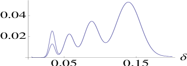
Figure 4: Power spectrum: dependence of height at the maximum on spreading width. The curve with the lower value of the most left maximum is identical to the one on the r.h.s. in Fig.2., while the higher peak is due to a decrease of its spreading width or an increase of its life time. Units as in Fig.2.

The folding (integration) of the cross section with the Morlet wavelet has to be done numerically. In order to obtain an analytic expression relating the number of fragmentations $f_{i}$ to the positions of the maxima of the power spectrum, we consider an expansion of a cross section into a Fourier series

$$\frac{{\rm d}\sigma(\omega)}{{\rm d}\Omega}=\sum_{m}c_{m}\sin(m\pi\omega/I)+c_{0}$$ (6)

with the bulk term

$$c_{0}=\int\frac{{\rm d}\sigma(\omega)}{{\rm d}\Omega}\,{\rm d}\omega$$

(further terms with $\cos(m\pi\omega/I)$ are immaterial for the discussion). An intermediate structure manifests itself, if a few terms in (6) are appreciably stronger than the others. In Fig.2 the terms with $c_{12}\approx c_{22}\approx c_{34}\approx c_{58}$ are dominant; of course, terms for different $m$-values also occur but are smaller by roughly an order of magnitude or more (here our analysis does not focus on $m\leq 4$: while giving larger contributions such values would correspond to $\delta\geq 0.5$ and represent gross and bulk structure). Performing analytically the wavelet-transform of each term in (6) (Mathematica gives a closed expression for the integral from which the formula below can be extracted), one obtains an analytic evaluation of the positions and heights of the maxima of the power spectrum. For each $\sin(m\pi x)$-term the positions of the local maxima in the power spectrum turn out to be

$${\rm Max}_{m}=\frac{k+\sqrt{2+k^{2}}}{2m\pi}I.$$ (7)

For $k=6$ (and the unity interval $I$) this yields 0.16, 0.088, 0.057 and 0.033 for $m=12,22,34$ and 58, respectively as verified in Fig.2. Note that a different choice of $k$ moves the positions of the local maxima, yet the $\sim 1/m$ law prevails. The expression (7) provides an obvious tool to be used to ascertain the number of fragmentations when the maxima are determined from an analysis of experimental data. Clearly, the number $f_{m}$ of fragmentations introduced above is related to the value $m$ in (6) by $m=2f_{m}$.

Furthermore, an increased value of $k$ can resolve a peak in the power spectrum that is caused by two near values of $f_{i}$. In fact, the distance between adjacent maxima (say $m=17$ and $m=18$) roughly doubles when $k$ is doubled.

While - for fixed $k$ - the $1/f_{i}$ dependence of the maxima of the power spectrum is an important finding, even more significant is the result that the values at the maxima (the heights) also obey the same $1/f_{i}$-law if the corresponding Fourier coefficients are about equal. Indeed, a straight line can be drawn through the maxima in Fig.2 as the four values $c_{m},\,m=12,22,34,58$ are about equal. We recall that, for example, $\sin(12\pi x)$ generates $f_{k}=6$ peaks of a width $\gamma_{k}=1/(2f_{k})$ in the energy (unit) interval for the cross section. This can be exploited in a realistic analysis: a deviation from this straight-line-rule signals effectively a deviation from the spreading width being assumed to be $1/(2f_{i})$. This is illustrated in Fig.4 where the spreading width $1/(2f_{4})$ has been decreased to $1/(2.8f_{4})$. As a result, the value of the first peak becomes enhanced. Since the spreading width is related to the life time of the states, we conclude: the life times are proportional to $f_{i}$ if the heights of the maxima lie on a straight line; an increased (decreased) height signals an even longer (shorter) life time.

In this context we note that the number of peaks and troughs in Fig.5 on the horizontal lines matches exactly the values of the $f_{i}$: six on the top, further down eleven, then seventeen and twenty nine on the bottom. The actual values of these peaks and troughs determine the heights of the bumps in the power spectrum, that is the information about the life times of the respective fragmented states. A similar wavelet transform obtained from experimental data is presented in Fig.8 (and 9) in Ref.dstadte, ; note that our schematic ’in vitro’ illustration is of course much more symmetric.

While in experiments the chaotic nature of the nucleus usually shows at higher excitation energies random , the pertinent structure revealed in the analysis may come as a surprise. We are of course familiar with order in the nuclear many body system as shown in shell effects and simple collective states. The fragmentations of the QR may be due to a different quality: it could be a manifestation of self-organising structures bak ; nil ; sor . Indeed, the life-time of increasingly complex configurations of the QR is increasing toward the compound states and the ground state. There is no general accepted definition of conditions under which the self-organising structures are expected to arise. We may speculate that in the case considered here, once the nuclear QR state is created, it is driven to an unstable hierarchy of configurations (metastable states) by quantum selection rules which connect these different complex configurations due to internal mixing. This problem needs of course a dedicated study on its own and is beyond the scope of the present paper.

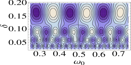
Figure 5: Wavelet contour plot of cross section shown in Fig.2. The symbols $\delta$ and $\omega_{0}$ refer to the Morlet wavelet parameters used in (5). The (positive) maxima are in light shading and the (negative) minima in dark. For the top pattern the contours range from 0.4 to $-0.4$.

We summarise the major points of our findings: (i) the position of the peaks in the power spectrum indicate the number of fragmentations of a particular intermediate state; the more complex states lie to the left of the simpler states (see Eq.(7)); (ii) the resolution of poorly resolved peaks can be improved by a higher value of $k$; (iii) the values (heights) at the peaks are related to the spreading widths, implying knowledge about the life times: if they lie on a straight line, the life times are proportional to the number of fragmentations, if they lie above (below) the straight line the corresponding life times are longer (shorter). Finally, we mention that a pronounced gross structure of the experimental cross section as found in lighter nuclei, would have no effect upon our findings. In fact, such gross structure had to occur at the far right end (values of $\delta$ appreciably larger than those used in the literature) of the power spectrum.

I Acknowledgement

WDH is thankful for the hospitality which he received from the Nuclear Theory Section of the Bogoliubov Laboratory, JINR during his visit to Dubna. The authors gratefully acknowledge enlightening discussions with J. Carter, R. Fearick and P. von Neumann-Cosel. This work is partly supported by JINR-SA Agreement on scientific collaboration, by Grant No. FIS2008-00781/FIS (Spain) and RFBR Grants No. 08-02-00118 (Russia).

References

- (1) M. N. Harakeh and A. van der Woude, Giant Resonances: Fundamental High-Frequency Modes of Nuclear Excitation (Clarendon Press, Oxford, 2001).
- (2) A. Bohr and B. R. Mottelson, Nuclear Structure, v.II (World Scientific, Singapore, 1998).
- (3) P. Ring and P. Schuck, The Nuclear Many-Body Problem (Springer-Verlag, New York, 1980).
- (4) R. Lauritzen, F. P. Bortignon, R. A. Broglia, and V. G. Zelevinsky, Phys. Rev. Lett. 74, 5190 (1995).
- (5) V. V. Sokolov and V. G. Zelevinsky, Phys. Rev. C56, 311 (1997).
- (6) H. Aiba and M. Matsuo, Phys. Rev. C60, 034307 (1999).
- (7) D. Lacroix and P. Chomaz, Phys. Rev. C60, 064307 (1999).
- (8) A. Shevchenko, J. Carter, R. W. Fearick, S. V. Förtsch, H. Fujita, Y. Fujita, Y. Kalmykov, D. Lacroix, J. J. Lawrie, P. von Neumann-Cosel, R. Neveling, V. Yu. Ponomarev, A. Richter, E. Sideras-Haddad, F. D. Smit, and J. Wambach, Phys. Rev. Lett. 93, 122501 (2004).
- (9) A. Shevchenko, G. R. J. Cooper, J. Carter, R. W. Fearick, Y. Kalmykov, P. von Neumann-Cosel, V. Yu. Ponomarev, A. Richter, I. Usman and J. Wambach, Phys. Rev. C77, 024302 (2008).
- (10) A. Shevchenko, O. Burda, J. Carter, G. R. J. Cooper, R. W. Fearick, S. V. Förtsch, Y. Fujita, Y. Kalmykov, D. Lacroix, J. J. Lawrie, P. von Neumann-Cosel, R. Neveling, V. Yu. Ponomarev, A. Richter, E. Sideras-Haddad, F. D. Smit, and J. Wambach, Phys. Rev. C79, 044305 (2009).
- (11) I. Daubechies, Ten Lectures on Wavelets, SIAM, Vol.61 (1992).
- (12) S. Mallat, A Wavelet Tour of Signal Processing (Academic Press, San Diego, 1998).
- (13) H. L. Resnikoff and R. O. Wells Jr., Wavelet Analysis: The Scalable Structure of Information (Springer-Verlag, New York, 2002).
- (14) J.-P. Blaizot and G. Ripka, Quantum Theory of Finite Systems (The MIT Press, London, 1986).
- (15) F. J. W. Hahne and W. D. Heiss, Ann. Phys. 89, 68 (1975).
- (16) T. Guhr, A. Müller-Groeling, and H. Weidenmüller, Phys. Rep. 299, 189 (1998); H. A. Weidenmüller and G. E. Mitchell, Rev. Mod. Phys. 81, 539 (2009).
- (17) P. Vesely, J. Kvasil, V. O. Nesterenko, W. Kleinig, P.-G. Reinhard, and V. Yu. Ponomarev, Phys. Rev. C80, 031302(R) (2009); C. L. Bai, H. O. Zhang, X. Z. Zhang, F. R. Xu, H. Sagawa, and G. Coló, Phys. Rev. C79, 041301(R) (2009).
- (18) P. Bak, C. Tang, and K.Wiesenfeld, Phys. Rev. Lett. 59, 381 (1987).
- (19) H. J. Jensen, Self-Organized Criticality: Emergent Complex Behaviour in Physical and Biological Systems (Cambridge University Press, Cambridge, 1998).
- (20) D. Sornette, Critical Phenomena in Natural Sciences. Chaos, Fractals, Selforganization and Disorder: Concepts and Tools (Springer, Berlin, 2000).