Convergence of expansions in Schrödinger and Dirac eigenfunctions, with an application to the $R$-matrix theory

Abstract

Expansion of a wave function in a basis of eigenfunctions of a differential eigenvalue problem lies at the heart of the $R$-matrix methods for both the Schrödinger and Dirac particles. A central issue that should be carefully analyzed when functional series are applied is their convergence. In the present paper, we study the properties of the eigenfunction expansions appearing in nonrelativistic and relativistic $R$-matrix theories. In particular, we confirm the findings of Rosenthal [J. Phys. G 13, 491 (1987)] and Szmytkowski and Hinze [J. Phys. B 29, 761 (1996); J. Phys. A 29, 6125 (1996)] that in the most popular formulation of the $R$-matrix theory for Dirac particles, the functional series fails to converge to a limit claimed by other authors.

I Introduction

Convergence of expansions of a one-component function into a series of eigenfunctions of a Sturm–Liouville problem was a subject of many studies. In some physical situations WignerEisenbud ; SturmLiouville_applications , of particular interest are expansions of a function defined only on a finite and closed interval. The classical results on convergence of such series can be found, for instance, in SturmLiouville_applications, ; Titchmarsh, ; LevitanSargsjan, ; CoddingtonLevinson, ; Atkinson, and for modern studies on this type of problems, including the equiconvergence method, the reader is referred to Minkin, ; Mityagin_Schrodinger, and references therein.

A similar problem for a two-component function was addressed by a number of mathematicians at the beginning of the 20th century Hurwitz ; Camp ; Schur ; BirkhoffLanger ; Bliss ; Titchmarsh_art and later reviewed in numerous textbooks (see e.g. LevitanSargsjan, ; CoddingtonLevinson, ; Atkinson, ). However, very few articles and textbooks deal with the development of an arbitrary function on a closed interval. Usually, either the expansion on an open interval is studied only Camp ; Titchmarsh_art or some additional conditions are imposed on the expanded function at the boundary pointsHurwitz ; Camp ; Schur ; Bliss . To the best of the author’s knowledge, the only classical paper discussing the general situation is the one by Birkhoff and Langer BirkhoffLanger . A more recent analysis of this kind of problems can be found, e.g., in Mityagin_Dirac, . A generalization of the equiconvergence method Minkin to a vector case should be also possible.

In the present paper, we apply the general results concerning convergence of eigenfunction expansions in the context of the $R$-matrix theory of scattering processes. This theory was first developed for low-energy collisions that could be described with the Schrödinger equation WignerEisenbud (see ThomasLane, ; Barrett, ; Szmytkowski_rev, for reviews on the subject). The $R$-matrix theory for the Dirac equation Goertzel was formulated soon after the nonrelativistic one, with nuclear applications in view. Only later it was realized that the electron–atom collisions involving targets with large atomic numbers require a Dirac description, due to the increasing role of relativistic effects. The $R$-matrix theory was reinvestigated in this context in Chang, .

The central idea in the formulation of the $R$-matrix methods for scattering from spherically symmetric potentials is to divide the whole space into two regions, a finite reaction volume $r<\varrho$ and the outer region $r\geq\varrho$, and to expand a wave function in the inner region in a series of eigenfunctions of the Hamiltonian governing the scattering process augmented, however, by artificial boundary conditions at the sphere $r=\varrho$. This procedure allows one to express the $R$-matrix as a limit $r\to\varrho^{-}$ of an infinite functional series. In both nonrelativistic and relativistic theories the critical issue, the convergence of the series on the boundary, was not properly analyzed by the originators and only presumed to hold. The convergence question was first recognized by Rosenthal Rosenthal , however his conclusions were incorrect. Later Szmytkowski and Hinze SzmytkowskiHinze1995 ; SzmytkowskiHinze1996 ; Szmytkowski1998 realized that while the development of the solution in the Schrödinger formulation converges in the whole interval to an expanded function, the analogous series appearing in the relativistic case has a discontinuity at the crucial boundary point. In this way, in the most popular formulation of the method, the solution depends on the artificial boundary condition imposed on the basis functions. Taking this into account, Szmytkowski and Hinze developed the correct Dirac $R$-matrix theory. Their conclusion caused much controversy Grant_last and was not widely recognized by the community Grant_book ; Burke_book . We present here a theorem confirming their resultsSzmytkowskiHinze1995 ; SzmytkowskiHinze1996 ; Szmytkowski1998 as well as the general result on convergence obtained by Szmytkowski JMathPhys .

The paper is organized as follows. In Section II, we recall basic facts from both nonrelativistic and relativistic $R$-matrix theories to highlight the problem of convergence appearing in both of them. In Section III, we give the general convergence theorems concerning the eigenfunction expansions Titchmarsh ; BirkhoffLanger . The main result of the paper, a solution to the Dirac $R$-matrix puzzle based on the theorem by Birkhoff and Langer BirkhoffLanger , can be found in Section III. We finish the paper with conclusions and point out some open problems.

II Expansions appearing in the $R$-matrix theories

The nonrelativistic and relativistic theories share many similarities, however in one essential point they are very different, i.e. the eigenfunction expansion of the solution of a nonrelativistic wave equation converges to a continuous function, whereas an analogous series in the relativistic theory has a discontinuity at the crucial boundary point SzmytkowskiHinze1995 ; SzmytkowskiHinze1996 ; JMathPhys . As a result, the relativistic $R$-matrix is not appropriately expressed by a functional series. To highlight this difference, we shortly introduce both methods in a single-channel scattering from spherically symmetric potentials. The notation used in the following sections is based on the monograph on the $R$-matrix methods in scattering Szmytkowski_rev .

II.1 Nonrelativistic $R$-matrix theory

A nonrelativistic elastic scattering process of spinless particles with mass $m$ and energy $E>0$ from a spherically symmetric potential $V(r)$ is governed by the stationary Schrödinger equation. We assume that the potential $V(r)$ affects the particle only in a finite spherical volume of radius $\varrho$ centered at $r=0$, denoted further by $\mathcal{V}_{\varrho}$. Outside this (inner) region the particle is free and its wave function satisfies the free-Hamiltonian stationary Schrödinger equation. Obviously, the solution in the inner region must pass smoothly into the solution in the outer region. We denote by $\Psi(E,\mathbf{r})$ the wave function being the solution of the respective Schrödinger equations in the inner and outer regions.

Since the potential is spherically symmetric, it is enough to consider only the radial part of the function $\Psi(E,\mathbf{r})$ corresponding to the multiindex $\gamma=(l,m_{l})$. For a general function $f(\mathbf{r})$, it is defined as

$$F_{\gamma}(r)=\int_{4\pi}\mathrm{d}\mathbf{\hat{r}}r^{2}\Upsilon_{\gamma}(\mathbf{r})f(\mathbf{r}),\quad\mathbf{\hat{r}}=\frac{\mathbf{r}}{r},$$ (1)

where $\Upsilon_{\gamma}(\mathbf{r})=(1/r)\mathrm{i}^{l}Y_{\gamma}(\mathbf{\hat{r}})$, and $Y_{\gamma}$ are normalized spherical harmonics defined as in CondonShortley, . We denote by $\boldsymbol{P}(E,r)$ a vector of radial functions of $\Psi(E,\mathbf{r})$ with elements $P_{\gamma}(E,r)$, and by $\boldsymbol{D}(E,r)$ a vector of radial functions of $\mathbf{\hat{r}}\cdot\boldsymbol{\nabla}\Psi(E,\mathbf{r})$ with elements $D_{\gamma}(E,r)$. Let us assume that there exists a matrix $\mathsf{R}_{\mathsf{b}}(E,\varrho)$ connecting $\boldsymbol{P}(E,r)$ and $\boldsymbol{D}(E,r)$ on the boundary of $\mathcal{V}_{\varrho}$ (which on the radial grid corresponds to $r=\varrho$) in the following way:

$$\boldsymbol{P}(E,\varrho)=\mathsf{R}_{\mathsf{b}}(E,\varrho)[\boldsymbol{D}(E,\varrho)-\mathsf{b}\boldsymbol{P}(E,\varrho)],$$ (2)

where $\mathsf{b}$ is an arbitrary square matrix. The above relation defines the $R$-matrix $\mathsf{R}_{\mathsf{b}}(E,\varrho)$. In what follows, it will be assumed that $\mathsf{b}$ is a diagonal, energy-independent, real matrix. Then the $R$-matrix is also diagonal, and its elements will be denoted by $(\mathsf{R}_{\mathsf{b}})_{\gamma\gamma}\equiv\mathsf{R}_{\mathsf{b}\gamma}$. Finding the $R$-matrix is equivalent to solving the scattering problem since $\mathsf{R}_{\mathsf{b}}(E,\varrho)$ is simply connected to the scattering matrix Szmytkowski_rev .

To determine the eigenfunction expansion of the $R$-matrix, we consider the radial part of the Schrödinger equation in the inner region $\mathcal{V}_{\varrho}$:

$$\left(-\frac{\hslash^{2}}{2m}\frac{\mathrm{d}^{2}}{\mathrm{d}r^{2}}+\frac{\hslash^{2}l(l+1)}{2mr^{2}}+V(r)-E\right)P_{\gamma}(E,r)=0,\quad r\in[0,\varrho).$$ (3)

We emphasize that here we do not make any restrictions on the function, except that it vanishes at $r=0$ as $r^{l+1}$. Our aim is to expand the unknown radial function $P_{\gamma}(E,r)$ in the basis $\{P_{i}^{(\gamma)}(r)\}$ generated by the same Hamiltonian, but augmented by the artificial boundary condition at $r=\varrho$, that is

$$\left(-\frac{\hslash^{2}}{2m}\frac{\mathrm{d}^{2}}{\mathrm{d}r^{2}}+\frac{\hslash^{2}l(l+1)}{2mr^{2}}+V(r)-E_{i}\right)P_{i}^{(\gamma)}(r)=0,\quad r\in[0,\varrho],$$ (4)

$$\lim_{r\to 0}r^{-l-1}P_{i}^{(\gamma)}(r)=\mathrm{const},\qquad\frac{\mathrm{d}}{\mathrm{d}r}P_{i}^{(\gamma)}(r)\Big{|}_{r=\varrho}=\left(\mathsf{b}_{\gamma\gamma}+\frac{1}{\varrho}\right)P_{i}^{(\gamma)}(\varrho).$$ (5)

The set of eigenvalues $E_{i}$ is countably infinite, and eigenfunctions corresponding to different eigenvalues are orthogonal under the standard scalar product in $\mathcal{L}^{2}([0,\varrho])$. The formal expansion of an arbitrary function on $[0,\varrho]$ is

$$P_{\gamma}(E,r)=\sum_{i=0}^{\infty}C_{i}(E)P_{i}^{(\gamma)}(r),\qquad C_{i}(E)=\int_{0}^{\rho}\mathrm{d}rP_{i}^{(\gamma)}(r)P_{\gamma}(E,r),$$ (6)

where we assume that the functions $\{P_{i}^{(\gamma)}\}$ are normalized to unity. The choice of the boundary conditions (5) for the basis functions allows us to write the coefficient $C_{i}(E)$ in a form that reveals the proportionality to $D_{\gamma}(E,\varrho)-\mathsf{b}_{\gamma\gamma}P_{\gamma}(E,\varrho)$ [compare to equation (2)]. In the case that we consider it holds that $D_{\gamma}(E,r)=r\partial_{r}(1/r)P_{\gamma}(E,r)$. Using equations (3) and (4) and the boundary conditions fulfilled by $P_{i}^{(\gamma)}(r)$, we obtain

$$P_{\gamma}(E,r)=\frac{\hslash^{2}}{2m}[D_{\gamma}(E,\varrho)-\mathsf{b}_{\gamma\gamma}P_{\gamma}(E,\varrho)]\sum_{i=0}^{\infty}\frac{P_{i}^{(\gamma)}(\varrho)}{E_{i}-E}P_{i}^{(\gamma)}(r),\quad r\in[0,\varrho).$$ (7)

Taking the limit $r\to\varrho^{-}$ on both sides leads to

$$P_{\gamma}(E,\varrho)=\mathsf{R}_{\mathsf{b}\gamma}(E,\varrho)[D_{\gamma}(E,\varrho)-\mathsf{b}_{\gamma\gamma}P_{\gamma}(E,\varrho)],$$ (8)

where

$$\mathsf{R}_{\mathsf{b}\gamma}(E,\varrho)=\frac{\hslash^{2}}{2m}\lim_{r\to\varrho^{-}}\sum_{i=0}^{\infty}\frac{P_{i}^{(\gamma)}(\varrho)P_{i}^{(\gamma)}(r)}{E_{i}-E}.$$ (9)

Comparing equations (8) and (2) we see that equation (9) defines a diagonal element of the $R$-matrix $\mathsf{R}_{\mathsf{b}}$. One notices that the $R$-matrix is expressed as a continuous extension of a functional series to the point $r=\varrho$. The main question that we are going to answer in section 3 is: Can one interchange the symbols of limit and sum, and still obtain the same result? In other words, does the series on the right-hand side of equation (9) converge to a continuous function in $[0,\varrho]$?

II.2 Relativistic $R$-matrix theory

The relativistic description of an elastic scattering process for particles of spin $\frac{1}{2}$ with rest mass $m$ and total energy $E$ ($|E|>mc^{2}$) is governed by the stationary Dirac equation. Similarly as we have done in the nonrelativistic case, we assume that the potential $V(r)$ vanishes outside the spherical volume $\mathcal{V}_{\varrho}$ bounded by a spherical shell, corresponding on the radial grid to $r=\varrho$, and that the wave functions $\boldsymbol{\Psi}(E,\mathbf{r})$ in the inner and outer regions pass smoothly one into the other on the boundary of $\mathcal{V}_{\varrho}$. To define the relativistic $R$-matrix, we fix the following notation:

$$\Omega_{\gamma}^{(+)}(\mathbf{r})=\frac{1}{r}\left(\!\!\begin{array}[]{c}\mathrm{i}^{l}\Omega_{\kappa m_{j}}(\mathbf{\hat{r}})\\ 0\end{array}\!\!\right),\quad\Omega_{\gamma}^{(-)}(\mathbf{r})=\frac{1}{r}\left(\!\!\begin{array}[]{c}0\\ \mathrm{i}^{l+1}\Omega_{-\kappa m_{j}}(\mathbf{\hat{r}})\end{array}\!\!\right),$$ (10)

where the multiindex $\gamma$ is defined as $(\kappa,m_{j})$, with $\kappa\in\mathbbm{Z}\setminus\{0\}$ and $m_{j}=\{-|\kappa|+1/2,-|\kappa|+3/2,\ldots,|\kappa|-1/2\}$, $l=|\kappa+1/2|-1/2$, and $\Omega_{\pm\kappa m_{j}}(\hat{\mathbf{r}})$ are the spherical spinors Szmytkowski_spinors . We define two radial functions of a four-component vector $\mathbf{f}(\mathbf{r})$, denoted by the superscripts $\pm$. For a fixed multiindex $\gamma$ they are given by

$$F_{\gamma}^{(\pm)}(r)=\int_{4\pi}\mathrm{d}\mathbf{\hat{r}}r^{2}\Omega_{\gamma}^{(\pm)\dagger}(\mathbf{r})\mathbf{f}(\mathbf{r}).$$ (11)

We denote by $\boldsymbol{P}(E,r)$ and $\boldsymbol{Q}(E,r)$ vectors of ”$+$” and ”$-$” radial functions of $\boldsymbol{\Psi}(E,\mathbf{r})$, respectively, with elements $P_{\gamma}(E,r)$ and $Q_{\gamma}(E,r)$. Let us define the $R$-matrix $\mathsf{R}_{\mathsf{b}}^{(+)}(E,\varrho)$ connecting $\boldsymbol{P}(E,r)$ and $\boldsymbol{Q}(E,r)$ on the surface of $\mathcal{V}_{\varrho}$ in the following way:

$$\boldsymbol{P}(E,\varrho)=\mathsf{R}_{\mathsf{b}}^{(+)}(E,\varrho)\left[\left(\frac{2mc}{\hslash}\right)\boldsymbol{Q}(E,\varrho)-\mathsf{b}\boldsymbol{P}(E,\varrho)\right],$$ (12)

where $\mathsf{b}$ is some square matrix. Henceforward we will assume $\mathsf{b}$ to be diagonal, energy-independent and real. In this case the $R$-matrix will be diagonal as well.

To find the $R$-matrix, we consider the radial part of the Dirac equation in the internal region $\mathcal{V}_{\varrho}$:

$$\left(\begin{array}[]{cc}mc^{2}+V(r)-E&c\hslash(-\mathrm{d}/\mathrm{d}r+\kappa/r)\\ c\hslash(\mathrm{d}/\mathrm{d}r+\kappa/r)&-mc^{2}+V(r)-E\end{array}\right)\left(\begin{array}[]{c}P_{\gamma}(E,r)\\ Q_{\gamma}(E,r)\end{array}\right)=0,\quad r\in[0,\varrho).$$ (17)

Since the solution must fulfill some unknown boundary condition, given by (12), at the point $r=\varrho$, we do not make any assumptions on the functions $P_{\gamma}(E,r)$ and $Q_{\gamma}(E,r)$, except for that they vanish for $r=0$. Note that equation (17) is a homogeneous differential equation in which $E$ is a parameter, and not an eigenvalue problem. We will expand the unknown solution in the basis generated by the eigenproblem consisting of the Dirac Hamiltonian of the previous equation and boundary conditions that, though unphysical, will allow us to develop the $R$-matrix into a functional series. Let us consider the eigenproblem

$$\left(\!\!\begin{array}[]{cc}mc^{2}+V(r)-E_{i}&\!\!c\hslash(-\mathrm{d}/\mathrm{d}r+\kappa/r)\\ c\hslash(\mathrm{d}/\mathrm{d}r+\kappa/r)&\!\!-mc^{2}+V(r)-E_{i}\end{array}\!\!\right)\left(\!\!\begin{array}[]{c}P_{i}^{(\gamma)}(r)\\ Q_{i}^{(\gamma)}(r)\end{array}\!\!\right)=0,\quad r\in[0,\varrho],$$ (22)

$$\lim_{r\to 0}r^{-\nu}P_{i}^{(\gamma)}(r)=\mathrm{const},\qquad Q_{i}^{(\gamma)}(\varrho)=(2mc/\hslash)^{-1}\mathsf{b}_{\gamma\gamma}P_{i}^{(\gamma)}(\varrho),$$ (23)

where $\nu=l+1$ if $V(0)=\mathrm{const}$, and $\nu=\sqrt{\kappa^{2}-(\alpha Z)^{2}}$ for the Coulomb potential ($\alpha$ is the fine-structure constant and $Z$ the atomic number). The set of real eigenvalues $\{E_{i}\}$ is infinitely countable. Moreover, the eigenfunctions corresponding to different eigenvalues are orthogonal in the sense

$$\int_{0}^{\varrho}\mathrm{d}r\big{(}P_{i}^{(\gamma)}(r),Q_{i}^{(\gamma)}(r)\big{)}\left(\begin{array}[]{c}P_{j}^{(\gamma)}(r)\\ Q_{j}^{(\gamma)}(r)\end{array}\right)=\mathcal{N}_{i}^{2}\delta_{ij}.$$ (24)

We will further assume the eigenfunctions to be normalized to unity; then the formal expansion of the functions $P_{\gamma}(E,r)$ and $Q_{\gamma}(E,r)$ is given by

$$\left(\begin{array}[]{c}P_{\gamma}(E,r)\\ Q_{\gamma}(E,r)\end{array}\right)=\sum_{i=-\infty}^{\infty}C_{i}(E)\left(\begin{array}[]{c}P_{i}^{(\gamma)}(r)\\ Q_{i}^{(\gamma)}(r)\end{array}\right),\quad r\in[0,\varrho),$$ (29)

$$C_{i}(E)=\int_{0}^{\varrho}\mathrm{d}r\Big{(}P_{i}^{(\gamma)}(r),Q_{i}^{(\gamma)}(r)\Big{)}\left(\begin{array}[]{c}P_{\gamma}(E,r)\\ Q_{\gamma}(E,r)\end{array}\right).$$ (32)

The coefficients $C_{i}(E)$ can be written in the form revealing the connection to the $R$-matrix. Using equations (17) and (22) and the boundary conditions fulfilled by $P_{i}^{(\gamma)}(r)$, we obtain

$$\left(\!\!\begin{array}[]{c}P_{\gamma}(E,r)\\ Q_{\gamma}(E,r)\end{array}\!\!\right)=\frac{\hslash^{2}}{2m}\left[\frac{2mc}{\hslash}Q_{\gamma}(E,\varrho)-\mathsf{b}_{\gamma\gamma}P_{\gamma}(E,\varrho)\right]\!\sum_{i=-\infty}^{\infty}\!\frac{P_{i}^{(\gamma)}(\varrho)}{E_{i}-E}\left(\!\!\begin{array}[]{c}P_{i}^{(\gamma)}(r)\\ Q_{i}^{(\gamma)}(r)\end{array}\!\!\right),\quad r\in[0,\varrho).$$ (37)

Taking the limit $r\to\varrho^{-}$ on both sides we obtain for the upper component

$$P_{\gamma}(E,\varrho)=\mathsf{R}_{\mathsf{b}\gamma}^{(+)}(E,\varrho)\left[\displaystyle{\frac{2mc}{\hslash}}Q_{\gamma}(E,\varrho)-\mathsf{b}_{\gamma\gamma}P_{\gamma}(E,\varrho)\right],$$ (38)

where

$$\mathsf{R}_{\mathsf{b}\gamma}^{(+)}(E,\varrho)=\frac{\hslash^{2}}{2m}\lim_{r\to\varrho^{-}}\sum_{i=-\infty}^{\infty}\frac{P_{i}^{(\gamma)}(\varrho)P_{i}^{(\gamma)}(r)}{E_{i}-E}\,.$$ (39)

Comparing equation (38) to equation (12), we see that (39) defines the diagonal elements of the $R$-matrix $\mathsf{R}_{\mathsf{b}}^{(+)}$. Exactly as in the case of the nonrelativistic $R$-matrix (compare equation (9)), the relativistic $R$-matrix is expressed by a functional series whose convergence is directly related to the convergence properties of the series (29). In the relativistic case the same question arises: Does the interchange of the limit and the infinite sum in equation (39) still give the same result? In other words, does the following identity hold:

$$\lim_{r\to\varrho^{-}}\sum_{i=-\infty}^{\infty}\frac{P_{i}^{(\gamma)}(\varrho)P_{i}^{(\gamma)}(r)}{E_{i}-E} \stackrel{{\scriptstyle\Large{?}}}{{=}} \sum_{i=-\infty}^{\infty}\frac{P_{i}^{(\gamma)}(\varrho)P_{i}^{(\gamma)}(\varrho)}{E_{i}-E}\,?$$ (40)

The expression on the right-hand side of the above equation is traditionally called the $R$-matrix. However, in the next section we show that in the case of relativistic scattering it is not allowed to exchange the two operations. Therefore the “$R$-matrix” as defined on the right-hand side of equation (40) cannot connect the upper and lower component as in equation (12).

III Convergence theorems

In the previous section, we have reviewed the $R$-matrix theories for the Schrödinger and Dirac particles. In both cases the $R$-matrix has been defined as a limit of a certain eigenfunction expansion. In the nonrelativistic theory it is given by equation (9), whereas in the relativistic theory by equation (39). The problem of convergence of these two functional series is equivalent to convergence of expansions (6) and (29), respectively. Let us then recall the convergence theorems for these two problems starting with the one for the Schrödinger problem Titchmarsh .

Theorem 1.

(adapted from Ref. Titchmarsh, ) Consider the set of solutions of the following Sturm–Liouville problem:

$$\left[-\frac{\mathrm{d}^{2}}{\mathrm{d}x^{2}}+q(x)-\lambda_{n}\right]y_{n}(x)=0,\qquad a\leq x\leq b,$$ (41)

$$\left\{\begin{array}[]{l}y_{n}(a)\cos\alpha+y_{n}^{\prime}(a)\sin\alpha=0\\ y_{n}(b)\cos\beta+y_{n}^{\prime}(b)\sin\beta=0\end{array}\right.,$$ (44)

where $q$ is assumed to be a real continuous function, and $\alpha,\beta\in[0,\pi)$. Suppose now that $f$ is a real, continuous function of bounded variation in the interval $[a,b]$. Then the expansion of $f$ in the eigenfunctions of the eigenproblem (41)+(44) reads:

$$\bar{f}(x)=\sum_{n=0}^{\infty}c_{n}y_{n}(x),$$ (45)

with

$$c_{n}=\int_{a}^{b}\mathrm{d}x\,y_{n}(x)f(x),$$ (46)

where the eigenfunctions $y_{n}$ are assumed to be normalized to unity in $\mathcal{L}^{2}([a,b])$. The series $\bar{f}(x)$ converges uniformly to $f(x)$ in the open interval $(a,b)$ [i.e., on each closed interval contained in $(a,b)$]. Moreover, for $x=a$ and $x=b$ the following relations are true:

$$\bar{f}(a)=\left\{\begin{array}[]{lc}f(a),&\mathrm{if}\,\alpha\neq 0\\ 0,&\mathrm{if}\,\alpha=0\end{array}\right.,\qquad\bar{f}(b)=\left\{\begin{array}[]{lc}f(b),&\mathrm{if}\,\beta\neq 0\\ 0,&\mathrm{if}\,\beta=0.\end{array}\right.$$ (47)

The above theorem can be applied to the nonrelativistic expansion, indicating that in equation (9) the limit can be exchanged with the infinite sum, giving

$$\mathsf{R}_{\mathsf{b}\gamma}(E,\varrho)=\frac{\hslash^{2}}{2m}\sum_{i=0}^{\infty}\frac{P_{i}^{(\gamma)}(\varrho)P_{i}^{(\gamma)}(\varrho)}{E_{i}-E}.$$ (48)

In what follows, we present a theorem concerning the expansion of a two component function appearing in the Dirac $R$-matrix definition.

Theorem 2.

(adapted from Ref. BirkhoffLanger, ) Consider the following boundary value problem:

$$\frac{\mathrm{d}}{\mathrm{d}x}\left(\begin{array}[]{c}u(x)\\ v(x)\end{array}\right)=\Big{[}\lambda A(x)+B(x)\Big{]}\left(\begin{array}[]{c}u(x)\\ v(x)\end{array}\right),\qquad a\leq x\leq b,$$ (53)

$$W_{a}\left(\begin{array}[]{c}u(a)\\ v(a)\end{array}\right)+W_{b}\left(\begin{array}[]{c}u(b)\\ v(b)\end{array}\right)=0,$$ (58)

where $A(x),B(x)$ are $2\times 2$ matrices of functions continuous with their first derivatives, $A(x)$ being diagonal, and $W_{a},W_{b}$ are constant $2\times 2$ square matrices. Let us assume that: (i) the eigenvalues of $A(x)$, denoted by $\vartheta_{j}(x)$ $(j=1,2)$, are continuous functions fulfilling the following conditions for all $x\in[a,b]$:

$$\vartheta_{j}(x)\neq 0$$

$$\vartheta_{1}(x)\neq\vartheta_{2}(x)$$

$$\mathrm{Arg}[\vartheta_{1}(x)-\vartheta_{2}(x)]=\mathrm{const}$$

$$\mathrm{Arg}\,\vartheta_{j}(x)=\mathrm{const}$$ (59)

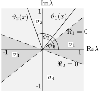
a) b)

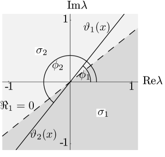
Figure 1: Two possible ways of dividing a complex plane of the parameter $\lambda$ into sectors in which the value $\Re_{j}$ has a fixed sign. In figure a) the two eigenvalues fulfill the condition $\mathrm{Arg}[\vartheta_{1}(x)]\neq\mathrm{Arg}[\pm\vartheta_{2}(x)]$ while in b) the two eigenvalues have phases differing by $\pi$, i.e., $\mathrm{Arg}[\vartheta_{1}(x)]=\mathrm{Arg}[-\vartheta_{2}(x)]$. The same division is given by the situation $\mathrm{Arg}[\vartheta_{1}(x)]=\mathrm{Arg}[\vartheta_{2}(x)]$, but it is not depicted in the figure to avoid repetition. The continuous halflines mark the rays on which the values of $\vartheta_{j}(x)$ lie, whereas the dashed lines — the rays on which the functions $\Re_{j}$ are equal to zero. The dashed lines are the borders of the sectors $\sigma_{k}$, $k=1,2,\ldots$.

Further, let us divide the complex plane of the parameter $\lambda$ into sectors in which the sign of the expressions $\Re_{j}=\mathrm{Re}(\lambda\int_{a}^{b}\mathrm{d}t\vartheta_{j}(t))$ $(j=1,2)$ is fixed. If one takes into account the conditions (2), there are two possibilities of dividing the complex plane of $\lambda$ corresponding to situations when either $\mathrm{Arg}[\vartheta_{1}(x)]\neq\mathrm{Arg}[\pm\vartheta_{2}(x)]$ or $\mathrm{Arg}[\vartheta_{1}(x)]=\mathrm{Arg}[\pm\vartheta_{2}(x)]$. Both divisions are visualized in figure 1, where the aforementioned sectors are denoted by $\sigma_{k}$, $k=1,2,\ldots$. For each sector $\sigma_{k}$ we define the $2\times 2$ matrices $\overline{\,\mathrm{I}}^{\,k}$ and $\underline{\,\mathrm{I}}^{\,k}$ with elements

$$(\overline{\,\mathrm{I}}^{\,k})_{ij}=\left\{\begin{array}[]{cc}\delta_{ij},&\Re_{j}\leq 0\,\;\mathrm{in\;sector}\;\sigma_{k}\\ 0,&\Re_{j}>0\,\;\mathrm{in\;sector}\;\sigma_{k}\end{array}\right.,$$ (62)

$$(\underline{\,\mathrm{I}}^{\,k})_{ij}=\left\{\begin{array}[]{cc}0,&\Re_{j}\leq 0\,\;\mathrm{in\;sector}\;\sigma_{k}\\ \delta_{ij},&\Re_{j}>0\,\;\mathrm{in\;sector}\;\sigma_{k}\end{array}\right..$$ (65)

(ii) Let the matrices $W_{a}$ and $W_{b}$ be such that in each sector $\sigma_{k}$ the following matrix is invertible:

$$\Omega_{k}\equiv W_{a}\overline{\,\mathrm{I}}^{\,k}+W_{b}\underline{\,\mathrm{I}}^{\,k}.$$ (66)

Then: 1. the set of eigenvalues $\lambda_{n}$ and respective normalized eigenfunctions $(u_{n},v_{n})^{T}$ of the problem (53)+(58) is infinitely countable; the orthonormality relation is the following:

$$\int_{a}^{b}\mathrm{d}x(\hat{u}_{n}(x),\hat{v}_{n}(x))A(x)\left(\begin{array}[]{c}u_{m}(x)\\ v_{m}(x)\end{array}\right)=\delta_{mn},$$ (67)

where $\big{(}\hat{u}_{n}(x),\hat{v}_{n}(x)\big{)}$ is the eigenvector of the adjoint boundary value problem footnote , corresponding to the eigenvalue $\lambda_{n}$. 2. the development of any two-component function $F=(F_{1},F_{2})^{T}$, real and continuous with the first derivative in the interval $[a,b]$, in the eigenfunctions of the boundary problem (53)+(58) is given by

$$\bar{F}(x)=\sum_{n=-\infty}^{\infty}C_{n}\left(\begin{array}[]{c}u_{n}(x)\\ v_{n}(x)\end{array}\right),$$ (68)

with

$$C_{n}=\int_{a}^{b}\mathrm{d}x\,\big{(}\hat{u}_{n}(x),\hat{v}_{n}(x)\big{)}A(x)\left(\begin{array}[]{c}F_{1}(x)\\ F_{2}(x)\end{array}\right).$$ (69)

The expansion (68) has the following properties:

$$\bar{F}(x) = F(x),\qquad\mathrm{for}\quad a<x<b,$$ (70a)

$$\bar{F}(a) = H_{a}F(a)+J_{a}F(b),$$ (70b)

$$\bar{F}(b) = H_{b}F(a)+J_{b}F(b),$$ (70c)

where the $2\times 2$ matrices $H_{a},J_{a},H_{b},J_{b}$ are fully determined by the matrix $A(x)$ and boundary conditions, and given by the expressions

$$H_{a} = \frac{1}{2}\mathbbm{1}_{2}+\sum_{k}\left[-\frac{\omega_{k}}{2\pi}\overline{\,\mathrm{I}}^{\,k}\Omega_{k}^{-1}W_{a}\underline{\,\mathrm{I}}^{\,k}\right]$$ (71a)

$$J_{a} = \sum_{k}\left[-\frac{\omega_{k}}{2\pi}\overline{\,\mathrm{I}}^{\,k}\Omega_{k}^{-1}W_{b}\overline{\,\mathrm{I}}^{\,k}\right]$$ (71b)

$$H_{b} = \sum_{k}\left[-\frac{\omega_{k}}{2\pi}\underline{\,\mathrm{I}}^{\,k}\Omega_{k}^{-1}W_{a}\underline{\,\mathrm{I}}^{\,k}\right]$$ (71c)

$$J_{b} = \frac{1}{2}\mathbbm{1}_{2}+\sum_{k}\left[-\frac{\omega_{k}}{2\pi}\underline{\,\mathrm{I}}^{\,k}\Omega_{k}^{-1}W_{b}\overline{\,\mathrm{I}}^{\,k}\right].$$ (71d)

In the above, the parameter $\omega_{k}$ is an angle between the boundary rays of a sector $\sigma_{k}$ (dashed lines in Fig. 1) and $\Omega_{k}$ is the invertible matrix defined in equation (66).

The above theorem is the special case of a more general eigenfunction expansion problem considered in BirkhoffLanger, . The reader may find there the proof of the above facts. We will present here in more details the situation directly applicable to the $R$-matrix expansion. Let us then state and prove the following corollary.

Corollary 1.

Consider the boundary value problem

$$\left(\!\begin{array}[]{cc}p(x)-\lambda\rho(x)&-\mathrm{d}/\mathrm{d}x+t(x)\\ \mathrm{d}/\mathrm{d}x+t(x)&q(x)-\lambda\rho(x)\end{array}\!\right)\left(\!\begin{array}[]{c}f(x)\\ g(x)\end{array}\!\right)=0,\quad a\leq x\leq b,$$ (76)

$$\left(\!\begin{array}[]{cc}\cos\alpha&\sin\alpha\\ 0&0\end{array}\right)\left(\begin{array}[]{c}f(a)\\ g(a)\end{array}\!\right)+\left(\!\begin{array}[]{cc}0&0\\ \cos\beta&\sin\beta\\ \end{array}\!\right)\left(\!\begin{array}[]{c}f(b)\\ g(b)\end{array}\!\right)=0,$$ (85)

with $p,q,t,\rho$ being real functions continuous with first derivatives, $\rho(x)>0$ for all $x\in[a,b]$ and $\alpha,\beta\in[0,\pi)$. Then the set of eigenvalues $\lambda_{n}$ and eigenfunctions $(f_{n},g_{n})^{T}$ is discrete. The expansion of a two-component function $F=(F_{1},F_{2})^{T}$, continuous with the first derivative in $[a,b]$, in the set $\{(f_{n},g_{n})^{T}\}$ is given by

$$\bar{F}(x)=\sum_{n=-\infty}^{\infty}C_{n}\left(\!\begin{array}[]{c}f_{n}(x)\\ g_{n}(x)\end{array}\!\right),$$ (88)

$$C_{n}=\int_{a}^{b}\mathrm{d}x\,\rho(x)\big{(}f_{n}(x),g_{n}(x)\big{)}\left(\!\begin{array}[]{c}F_{1}(x)\\ F_{2}(x)\end{array}\!\right),$$ (91)

and has the following properties:

$$\bar{F}(x) = F(x),\qquad\mathrm{for}\quad a<x<b,$$ (92a)

$$\bar{F}(a) = \frac{1}{2}\left(\!\begin{array}[]{ll}1-\cos 2\alpha&-\sin 2\alpha\\ -\sin 2\alpha&1+\cos 2\alpha\end{array}\!\right)F(a),$$ (92d)

$$\bar{F}(b) = \frac{1}{2}\left(\!\begin{array}[]{ll}1-\cos 2\beta&-\sin 2\beta\\ -\sin 2\beta&1+\cos 2\beta\end{array}\!\right)F(b).$$ (92g)

Proof.

To prove the corollary, let us rewrite equation (76) in such form that the results from BirkhoffLanger, , recalled in Theorem 2, apply directly, i.e. we would like to have the differential equation and boundary conditions in the form (53)+(58). To achieve this, we multiply equation (76) on the left-hand side by the unitary matrices $U$ and $\widetilde{U}$ given by

$$U=\frac{1}{\sqrt{2}}\left(\!\begin{array}[]{cc}\mathrm{i}&1\\ 1&\mathrm{i}\end{array}\!\right),\qquad\widetilde{U}=\left(\!\begin{array}[]{cc}\mathrm{i}&0\\ 0&-\mathrm{i}\end{array}\!\right),$$ (93)

obtaining

$$\frac{\mathrm{d}}{\mathrm{d}x}\left(\!\begin{array}[]{c}u(x)\\ v(x)\end{array}\!\right)=\left[\lambda\left(\!\begin{array}[]{cc}\mathrm{i}\rho(x)&0\\ 0&-\mathrm{i}\rho(x)\end{array}\!\right)+B(x)\right]\left(\!\begin{array}[]{c}u(x)\\ v(x)\end{array}\!\right),$$ (94)

where $u=(\mathrm{i}f+g)/\sqrt{2}$ and $v=(f+\mathrm{i}g)/\sqrt{2}$, the diagonal matrix on the right-hand side corresponds to the matrix $A$, and the matrix $B$ contains the functions $p,q,t$, and fulfills the assumptions of Theorem 2. At the same time, we have to adjust the boundary conditions to the functions $u$ and $v$. These become

$$\left(\!\begin{array}[]{cc}\mathrm{e}^{\mathrm{i}\alpha}&\mathrm{i}\mathrm{e}^{-\mathrm{i}\alpha}\\ -\mathrm{i}\mathrm{e}^{\mathrm{i}\alpha}&\mathrm{e}^{-\mathrm{i}\alpha}\end{array}\!\right)\left(\!\begin{array}[]{c}u(a)\\ v(a)\end{array}\!\right)+\left(\!\begin{array}[]{cc}-\mathrm{i}\mathrm{e}^{\mathrm{i}\beta}&\mathrm{e}^{-\mathrm{i}\beta}\\ \mathrm{e}^{\mathrm{i}\beta}&\mathrm{i}\mathrm{e}^{-\mathrm{i}\beta}\end{array}\!\right)\left(\!\begin{array}[]{c}u(b)\\ v(b)\end{array}\!\right)=0.$$ (95)

Comparing equation (95) to (58), we can see that the $2\times 2$ matrices on the left-hand side can be identified with $W_{a}$ and $W_{b}$, respectively. Let us then check if equation (94) with boundary conditions (95) satisfy the assumptions (i) and (ii) of Theorem 2.

First, we will find the division of the complex plane of the parameter $\lambda$ into sectors, as described in Theorem 2. The matrix $A(x)$ has two complex eigenvalues $\vartheta_{1}(x)=\mathrm{i}\rho(x)$ and $\vartheta_{2}(x)=-\mathrm{i}\rho(x)$. Note that since $\rho(x)$ is strictly greater than zero and continuous for all $x\in[a,b]$, they satisfy the condition (i) of Theorem 2. Note, in particular, that $\mathrm{Arg}[\vartheta_{1}(x)]=\mathrm{Arg}[-\vartheta_{2}(x)]$, which leads to the division of the complex plane of the type shown in Figure 1b, i.e. we have the following two sectors:

$$\sigma_{1}=\{\lambda:\Re_{1}<0\wedge\Re_{2}>0\}=\{\lambda:\mathrm{Im}\,\lambda\geq 0\}$$ (96)

and

$$\sigma_{2}=\{\lambda:\Re_{1}>0\wedge\Re_{2}<0\}=\{\lambda:\mathrm{Im}\,\lambda<0\}.$$ (97)

This implies that the matrices defined in (62) are

$$\overline{\,\mathrm{I}}^{\,1}=\left(\!\begin{array}[]{cc}1&0\\ 0&0\\ \end{array}\!\right), \underline{\,\mathrm{I}}^{\,1}=\left(\!\begin{array}[]{cc}0&0\\ 0&1\\ \end{array}\!\right),$$ (102)

$$\overline{\,\mathrm{I}}^{\,2}=\left(\!\begin{array}[]{cc}0&0\\ 0&1\\ \end{array}\!\right), \underline{\,\mathrm{I}}^{\,2}=\left(\!\begin{array}[]{cc}1&0\\ 0&0\\ \end{array}\!\right).$$ (107)

Now the condition (66) can be checked easily. Let us write out explicitly the matrices $\Omega_{1}$ and $\Omega_{2}$ for $W_{a}$ and $W_{b}$ as defined in (95), since we are going to use them in further calculations:

$$\Omega_{1}=\left(\!\begin{array}[]{cc}\mathrm{e}^{\mathrm{i}\alpha}&\mathrm{e}^{-\mathrm{i}\beta}\\ -\mathrm{i}\mathrm{e}^{\mathrm{i}\alpha}&\mathrm{i}\mathrm{e}^{-\mathrm{i}\beta}\\ \end{array}\!\right), \Omega_{2}=\left(\!\begin{array}[]{cc}-\mathrm{i}\mathrm{e}^{\mathrm{i}\beta}&\mathrm{i}\mathrm{e}^{-\mathrm{i}\alpha}\\ \mathrm{e}^{\mathrm{i}\beta}&\mathrm{e}^{-\mathrm{i}\alpha}\\ \end{array}\!\right).$$ (112)

Clearly, they are invertible for all values of $\alpha,\beta\in\mathbbm{R}$, so the condition (ii) from Theorem 2 is fulfilled.

We have checked that all assumptions of Theorem 2 are satisfied, therefore, the set $\{(u_{n},v_{n})^{T}\}$ of eigenfunctions of the problem (94)+(95) [and at the same time the set $\{(f_{n},g_{n})^{T}\}$ of eigenfunctions of the problem (76)+(85)] is countably infinite. Moreover, part 2 of the theorem applies to the expansion (88). To show explicitly that formulas (92a)–(92g) are valid, we premultiply equation (88) by $\sqrt{2}U$ obtaining the series of $(u_{n},v_{n})^{T}$ representing a complex two-component function $G=(G_{1},G_{2})^{T}=(F_{2}+\mathrm{i}F_{1},F_{1}+\mathrm{i}F_{2})^{T}$:

$$\bar{G}(x)=\sum_{n=-\infty}^{\infty}C_{n}\left(\!\begin{array}[]{c}u_{n}(x)\\ v_{n}(x)\end{array}\!\right).$$ (113)

Although part 2 of the theorem was formulated for real functions, the generalization to complex functions is straightforward if the real and imaginary parts are considered separately. Therefore, we will proceed with the complex function $G$. Notice that coefficients $C_{n}$ can be written as

$$C_{n} = \int_{a}^{b}\mathrm{d}x\,\rho(x)\big{(}f_{n}(x),g_{n}(x)\big{)}U^{\dagger}\widetilde{U}^{\dagger}\widetilde{U}U\left(\!\begin{array}[]{c}F_{1}(x)\\ F_{2}(x)\end{array}\!\right)$$ (116)

$$= \int_{a}^{b}\mathrm{d}x\,\big{(}\hat{u}_{n}(x),\hat{v}_{n}(x)\big{)}A(x)\left(\!\begin{array}[]{c}G_{1}(x)\\ G_{2}(x)\end{array}\!\right),$$ (119)

where $\big{(}\hat{u}_{n},\hat{v}_{n}\big{)}^{T}=(1/2)\widetilde{U}(u_{n},v_{n})^{T}$ is the solution of the eigenproblem adjoint to (94)+(95). The obtained formula for coefficients is in agreement with equation (69). Consequently, the series (88) modified with $U$ converges to expressions (70a), (70b), and (70c). Let us then determine the matrices $H_{a},J_{a},H_{b},J_{b}$ in this particular case. The angles $\omega_{1}$ and $\omega_{2}$ are equal to $\pi$ since the sectors $\sigma_{1(2)}$ are half-planes (see Figure 1b), so exploiting equations (71a)–(71d) we obtain

$H_{a}=\frac{1}{2}\left(\begin{array}[]{cc}1&-\mathrm{i}\mathrm{e}^{-2\mathrm{i}\alpha}\\ \mathrm{i}\mathrm{e}^{2\mathrm{i}\alpha}&1\end{array}\right),$	$H_{b}=\left(\begin{array}[]{ll}0&0\\ 0&0\end{array}\right),$
$J_{a}=\left(\begin{array}[]{ll}0&0\\ 0&0\end{array}\right),$	$J_{b}=\frac{1}{2}\left(\begin{array}[]{cc}1&-\mathrm{i}\mathrm{e}^{-2\mathrm{i}\beta}\\ \mathrm{i}\mathrm{e}^{2\mathrm{i}\beta}&1\end{array}\right).$

(120)

Taking into account the above results and equations (70b) and (70c), we obtain the following expressions for the sum of series (113) at the points $x=a$ and $x=b$:

$$\bar{G}(a)=H_{a}G(a),\qquad\bar{G}(b)=J_{b}G(b).$$ (121)

We recover the formulas for the original function $F$ premultiplying equations (121) with $(1/\sqrt{2})U^{\dagger}$:

$$\bar{F}(a)=U^{\dagger}H_{a}UF(a),\qquad\bar{F}(b)=U^{\dagger}J_{b}UF(b).$$ (122)

Finally, we insert the matrices (III) into the above equations and obtain slightly modified formulas (92d) and (92g):

$$\bar{F}(a) = \frac{1}{2}\left(\!\begin{array}[]{cc}2\sin^{2}\alpha&-\sin 2\alpha\\ -\sin 2\alpha&2\cos^{2}\alpha\end{array}\!\right)\left(\!\begin{array}[]{c}F_{1}(a)\\ F_{2}(a)\end{array}\!\right),$$ (123e)

$$\bar{F}(b) = \frac{1}{2}\left(\!\begin{array}[]{cc}2\sin^{2}\beta&-\sin 2\beta\\ -\sin 2\beta&2\cos^{2}\beta\end{array}\!\right)\left(\!\begin{array}[]{c}F_{1}(b)\\ F_{2}(b)\end{array}\!\right).$$ (123j)

Summarizing, in the open interval $(a,b)$ the series (88) converges to the function $F(x)$, whereas at the boundary points $x=a$ and $x=b$, the sum of the expansion is given by (123e) and (123j), respectively. This finishes the proof of Corollary 1. ∎

The Corollary reveals that the series (88) converges to the function $F(x)$ in the whole interval $[a,b]$ if and only if the following two equalities hold simultaneously:

$$\frac{1}{2}\left(\!\begin{array}[]{cc}2\sin^{2}\alpha&-\sin 2\alpha\\ -\sin 2\alpha&2\cos^{2}\alpha\end{array}\!\right)\left(\!\begin{array}[]{c}F_{1}(a)\\ F_{2}(a)\end{array}\!\right)=\left(\!\begin{array}[]{c}F_{1}(a)\\ F_{2}(a)\end{array}\!\right),$$ (130)

$$\frac{1}{2}\left(\!\begin{array}[]{cc}2\sin^{2}\beta&-\sin 2\beta\\ -\sin 2\beta&2\cos^{2}\beta\end{array}\!\right)\left(\!\begin{array}[]{c}F_{1}(b)\\ F_{2}(b)\end{array}\!\right)=\left(\!\begin{array}[]{c}F_{1}(b)\\ F_{2}(b)\end{array}\!\right),$$ (137)

which is equivalent to the condition

$$F_{1}(a)\cos\alpha+F_{2}(a)\sin\alpha=0,\qquad F_{1}(b)\cos\beta+F_{2}(b)\sin\beta=0.$$ (138)

One recognizes in this formulas the boundary conditions (85). Consequently, the sum of the series is continuous if and only if a function to be expanded fulfills the same boundary conditions as the basis functions.

We demonstrated in this section that the properties of the developments into eigensolutions of first-order differential systems (Theorem 2) and the expansions in the eigenfunctions of the Sturm–Liouville problem are dramatically different. This fact, not realized by the originators of the relativistic $R$-matrix method, has far-reaching consequences for the theory. Although the assumptions in Corollary 1 are restrictive, i.e. the functions $p,q,t,\rho$, being elements of the matrices appearing in the eigenproblem, are assumed to be continuous with their first derivative, its conclusion still can be applied to expansion (29) at the point $r=\varrho$. This can be done, because the boundary conditions are separated and, consequently, the convergence of the eigenfunction expansion at the point $r=\varrho$ is independent of the behaviour at the point $r=0$. In fact, one can consider the boundary-value problem (22)+(23) on the interval $[\varepsilon,\varrho]$ with the boundary condition $P_{i}^{(\gamma)}(\varepsilon)=0$ and show that the solution at the point $r=\varrho$ remains the same for an arbitrarily small $\varepsilon$. Taking this into account, we immediately see that the expansion (29) for $r=\varrho$ does not, in general, converge to the solution of (17). It does only if the functions $P_{\gamma}(E,r)$ and $Q_{\gamma}(E,r)$ satisfy the second of the boundary conditions (23). This, however, cannot be assumed since this particular condition does not have any physical meaning and is chosen in this way only to obtain the expansion of the $R$-matrix. As a result, the commonly used definition of the $R$-matrix contains an error, since in general it holds that

$$\lim_{r\to\varrho^{-}}\sum_{i=-\infty}^{\infty}\frac{P_{i}^{(\gamma)}(\varrho)P_{i}^{(\gamma)}(r)}{E_{i}-E} \boldsymbol{\neq} \sum_{i=-\infty}^{\infty}\frac{P_{i}^{(\gamma)}(\varrho)P_{i}^{(\gamma)}(\varrho)}{E_{i}-E}.$$ (139)

The way to correct this mistake was found by Szmytkowski and Hinze for a general multichannel case SzmytkowskiHinze1995 ; SzmytkowskiHinze1996 ; Szmytkowski_rev ; Szmytkowski1998 . They introduced the correction which should by subtracted from the common and faulty expression for the $R$-matrix in order to obtain the correct one.

IV Conclusion

Summarizing, we have provided theorems concerning the convergence of eigenfunction expansions of a two-component function into eigenfunctions of a Dirac operator on a finite closed interval augmented by separated boundary conditions. In particular, we have shown that such expansions have discontinuities at the boundary if the expanded function does not fulfill the same boundary conditions as the basis functions. This confirms the result of Szmytkowski JMathPhys and has far-reaching consequences for the relativistic $R$-matrix method. Moreover, the fact that the functional series does not, in general, converge to a continuous function in the closed interval may affect the rate of convergence and cause the Gibbs-like phenomenon Barkhudaryan1 ; Barkhudaryan2 to occur.

The issue left as an open problem is the proof of convergence of (88) in the case when the functions $p(x),q(x),t(x)$ have a singularity at one of the boundary points, e.g. at $x=a$. This is directly related to convergence of expansion (29) since the functions have discontinuities for $r=0$. However, due to the separated character of the boundary conditions (85) and the fact that both the expanded function and the basis functions vanish at $r=0$, the conclusions (92a) and (92g) of Corollary 1, which concern the point $r=\varrho$, should hold in this case, as well.