Optimal basis set for ab-initio calculations of energy levels in tunneling structures, using the covariance matrix of the wave functions

Abstract

The paper proposes a method to obtain the optimal basis set for solving the self consistent field (SCF) equations for large atomic systems in order to calculate the energy barriers in tunneling structures, with higher accuracy and speed. Taking into account the stochastic-like nature of the samples of all the involved wave functions for many body problems, a statistical optimization is made by considering the covariance matrix of these samples. An eigenvalues system is obtained and solved for the optimal basis set and by inspecting the rapidly decreasing eigenvalues one may seriously reduce the necessary number of vectors that insures an imposed precision. This leads to a potentially significant improvement in the speed of the SCF calculations and accuracy, as the statistical properties of a large number of wave functions in an large spatial domain may be considered. The eigenvalue problem has to be solved only few times, so that the amount of time added may be much smaller that the overall iterating SCF calculations.

A simple implementation of the method is presented for a situation where the analytical solution is known, and the results are encouraging.

1 Introduction

Ab initio methods become more and more efficient in various scientific and technical applications, as the involved physical principles, numerical methods and computer hardware display a constantly improvement. The whole effort is sustained by the big promises of these methods in the general field of the computer simulation of matter properties, with applications in physics, chemistry, biology, and many interdisciplinary scientific researches. However, there are still many problems that demand better solutions at any level of the ab initio methods and their solving is limited by the enormous computational effort implied by these kind of calculations even for the very small clusters of atoms that can be dealt today. As the large accessibility of supercomputers will be probably delayed for an unknown period and since there is a continuous need for larger atomic systems calculations, some progress is certainly needed in both physical principles (more accurate and elaborate models) and numerical methods (more precise and fast algorithms) to achieve this goal.

The physical part of this scenario has already an eight decade history, starting with the birth of the quantum mechanics. The Hartree method of the self consistent field (SCF) founded in the third decade of the last century was soon amended to include the exchange integral leading to the Hartree-Fock (HF) equations which still remain the least empirical way for ab initio calculations. Their well known expressions reveal the necessity of an iterating process, as each wave function depend on the others and they are present both under the differentiation and integration operators. Considering the Born Oppenheimer approximation, the left side of the equation for each particle is composed by the one electron term, the coulombian interaction between electrons and the exchange term due to spin:

$$\left[{-\frac{1}{2}\nabla^{2}+U\left(r\right)}\right]\Psi_{i}\left({\bf{r}}\right)+\sum\limits_{j}{\int{d{\bf{r}}{\rm{{}^{\prime}}}}\frac{{\left|{\Psi_{j}\left({{\bf{r}}{\rm{{}^{\prime}}}}\right)}\right|^{2}}}{{\left|{{\bf{r}}{\rm{-}}{\bf{r}}{\rm{{}^{\prime}}}}\right|}}\Psi_{i}\left({\bf{r}}\right)}$$ (1.1)

$$-\sum\limits_{j}{\delta_{s_{i},s_{j}}\int{d{\bf{r^{\prime}}}}}\frac{{\Psi_{j}^{*}\left({{\bf{r}}{\rm{{}^{\prime}}}}\right)\Psi_{i}\left({{\bf{r}}{\rm{{}^{\prime}}}}\right)}}{{\left|{{\bf{r}}{\rm{-}}{\bf{r}}{\rm{{}^{\prime}}}}\right|}}\Psi_{j}\left({\bf{r}}\right)=\varepsilon_{i}{\kern 1.0pt}\Psi_{i}\left({\bf{r}}\right)$$ (1.2)

where $\Psi_{i}\left({\rm{r}}\right)$ is the one electron wave function, $U\left(r\right)$ is the potential energy in the nucleus field, ${\bf{r}}$ and ${\bf{r}}^{\prime}$ are the vectors to the nucleus of the two electrons interacting and $s_{i}$ is the spin index. As usually, for the sake of simplicity, natural system units have been used in this equation

About three decades have been necessary for providing a solid theoretical base, in the framework of the Kohn-Sham (KS) formalism [1] of the Density Functional Theory (DFT) , for including the correlation term, and other decades for its satisfactory evaluation. Using the properties of an homogenous electron gas and introducing the functional of density, for a sufficiently slow varying density $n\left({\bf{r}}\right)=\sum\limits_{i=1}^{N}{\left|{\Psi_{i}\left({\bf{r}}\right)}\right|^{2}}$ , the system of equations reads [1]:

$$\left\{{-\frac{1}{2}\nabla^{2}+\varphi\left({\bf{r}}\right)+\mu_{c}\left({\bf{r}}\right)}\right\}\Psi_{i}\left({\bf{r}}\right)-\int{d{\rm{r}}^{\prime}\frac{{n_{1}\left({{\bf{r}}{\rm{,}}{\bf{r}}{\rm{{}^{\prime}}}}\right)}}{{\left|{{\bf{r}}{\rm{-}}{\bf{r}}{\rm{{}^{\prime}}}}\right|}}\Psi_{i}\left({{\bf{r}}{\rm{{}^{\prime}}}}\right)}=\varepsilon_{i}{\kern 1.0pt}\Psi_{i}\left({\bf{r}}\right)$$ (1.3)

where $\varphi\left({\bf{r}}\right)$ includes the one and two electrons potential, $\mu_{c}\left({\bf{r}}\right)$ includes the correlation effects and the last term of the left side of the equation is the new form of the exchange correction. Although theoretically more accurate than HF, the KS method has some necessary simplifying assumptions of the new parts of the model so that it is often considered slightly empirical in these aspects. For the most situations this formalism is highly efficient and the theoretical improved accuracy is present in many of the applications. However, probably due to its empirical part, it still fails sometimes, as HF also does in other situations due to the neglecting of the correlations.

Finally, it is worth to mention the existence of many other more or less empirical methods, with a greater speed, but with a more limited scope, with codes commercially available and widely used in various applications. As the physical model is still a rather simple one, refining the model is not expected to improve the speed of the ab initio calculations, but rather their accuracy.

Many other post HF models have appeared in the last decades, offering a multitude of choices for various aspects of the ab initio calculus. Thus, the exchange term may have several forms, as: exact HF exchange, Slater local exchange functional [2], Becke’s 1988 non-local gradient correction to exchange [3], Perdew-Wang 1991 generalized gradient approximation non-local exchange [4],[5]. For the correlation term the most accurate expressions seems to be: Vosko-Wilk-Nusair (VWN) local correlation functional [6], Perdew and Zunger’s 1981 local correlation functional [7], Lee-Yang-Parr non-local correlation functional [8], Perdew-Wang 1991 local correlation functional [4].

Concerning the numerical methods, the algorithms and the mathematics used in the ab initio calculations, there are many popular techniques that may be considered, each of them with their pros and cons [9]. Here the possibilities are more diversified, as the form of the self consistent equations may be purely differential or integro-differential, due to the exchange and correlation terms.

The differential form is often treated by the Numerov’s fifth order method, which is robust and accurate but is not self starting and require some initial iterations, as many other point by point methods of high order. A notable exception should be the forth order Runge-Kutta method but it is not well suited for boundary conditions equations as the HF ones. Some shooting method must accompany the point by point methods and, although this provides the eigenvalue of the equation (which sometimes is the main goal), it implies an iterating process that leads to a huge amount of computing effort. Furthermore, it must be used both for the wave function equation and for Poisson equation for finding the Hartree-Fock potential generated by the charge density.

An important step for improving the ab initio methods’ efficiency was made by Roothaan [10] who transferred the calculations to linear algebra in the form of a generalized eigenvalue problem, using non orthogonal basis set. The HF equations reduce to the following matrix equation which is more suitable for a numerical calculations:

$${\bf{FC=SC\varepsilon}}$$

where ${\bf{F}}$ is the Fock matrix, ${\bf{C}}$ is a matrix of coefficients of the two electrons interactions, ${\bf{S}}$ is the overlap matrix of the basis functions, and ${\bf{\varepsilon}}$ is the matrix of orbital energies. Thus, a class of new numerical techniques became eligible and an increasing interest for appropriate choosing of the basis set emerged.

Among the various methods with a reduced need of iterations that are currently used there are: finite difference method, finite element method, Galerkin method, collocation method, etc. The most promising class of methods for such boundary conditions equations is considered to be the class of spectral and pseudospectral methods [11], [12], as they have already been successfully used in various other fields. Their evanescence property (exponential decay of the error with the number of sampling points) and the absence of iteration processes are very attractive, but the main problem is the bad conditioning that often appears in the linear algebra implied. However, the matrix conditioning numbers are generally satisfactory if a low dimension of the vectorial space is chosen, but this tends to increase the errors if the basis set is not an optimal one.

We consider that the spectral methods in the ab initio calculations have not been entirely exploited, as even the basis sets seem to be still ”empirically” chosen: by subjective considerations (as Chebyshev polynomials are the usual basis of choice [11]), or artificial approximations that facilitate the analytical calculations with a great impact on the speed of the numerical part (for example the Gaussian basis). As the number of vectors used by a basis must be always finite and as small as possible to minimize the matrix condition number and the overall computational effort, the problem seems to be the choice of an optimum basis that provide the minimal error when the dimension of the vectorial space of the wave function representation is highly reduced.

In the next chapter we propose a method for properly choosing the basis set for achieving this minimization of the errors when dealing with a smaller number of vectors that is usually needed. An example for the implementation of the method will be later presented and some conclusions and further suggestions will be drawn.

2 The stochastic nature of the wave functions’ samples for many body problems

The radial wave function in a hydrogenoid atom, which is the primary natural approximation of the many body wave function has the well known form [13]:

$$R_{n\ell}\left(r\right)=\frac{2}{n^{2}}\sqrt{\frac{{\left({n-\ell-1}\right)!}}{{\left[\left({n+\ell}\right)!\right]^{3}}}}\left({\frac{{2r}}{n}}\right)^{\ell}e^{-\frac{r}{n}}L_{n-\ell-1}^{2\ell+1}\left({\frac{{2r}}{n}}\right)$$ (2.1)

where $n$ is the principal quantum number, $\ell$ is the angular momentum number, $r$ is the distance to the nucleus in Bohr radius and $L_{n}^{\ell}\left(r\right)$ are the associate Laguerre polynomials.

Every electron moving in the potential determined by the charge distribution created by such type of wave functions is thus influenced by all the others electrons. For systems with many electrons, the family of functions has the appearance shown in figure 1 (generated using Mathematica software). The asymptotic behavior of the wave functions allows one to deal with a finite interval, but this interval seems to be quite large for the usual methods for point to point differential equations . Thus, the errors are very important for most of the orbitals that imply distances above 15-20 Bohr radius, but the influence of the further regions is clearly present in the real system, and needs to be considered.

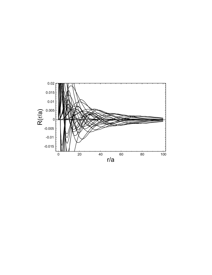
Figure 1: The various wave functions in a hydrogen-like atom for $n=1,2,...,7$

If one samples the distance to the nucleus, a pseudo-random distribution of the local values of these wave function appears as shown in figure 2.

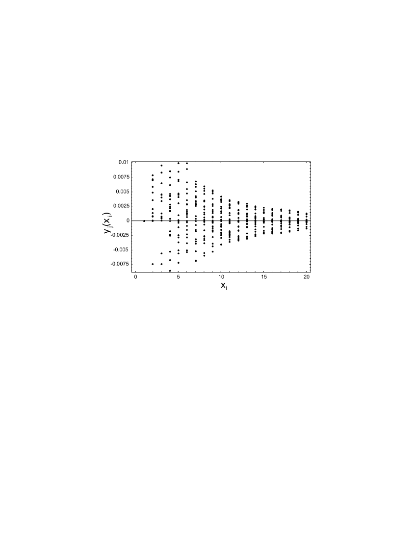
Figure 2: The equidistant samples of the wave functions in a hydrogen-like atom for $n=1,2,...,7$

Although the entropy displayed by these values is not very high, it is possible to consider a stochastic influence between the electrons, and use the second order statistic’s methods for dealing with them. The concept of the ”mean field”, with a clear stochastic connotation is present in many of the physical models accepted now-a-days but this context has not been considered enough in the present theories, except for some low order Monte-Carlo methods.

3 Using the Karhunen-Loeve theorem for calculating the optimum basis set

The spectral methods used for solving the eigenvalue problems in simple or generalized form, first approximate the solution as a linear combination of continuous functions - basis vectors- and then plug in this solution in the original equations to determine the coefficient matrix.

$$y\left(x\right)\approx\sum\limits_{i=0}^{N}{c_{i}\varphi_{i}\left(x\right)}$$ (3.1)

The domain of the independent variable is sampled in a number of points $x_{j}$ (as in the collocation method) where the equations are supposed to be satisfied, and the resulting linear system is solved for the coefficients.

$$y\left({x_{j}}\right)=\sum\limits_{i=0}^{N}{c_{i}\varphi_{i}\left({x_{j}}\right)},\quad j=0,...,N$$ (3.2)

As the values of $y\left(x\right)$ are known for the boundary points, a system of $N+1$ equations is obtained, and its solution gives the unknown coefficients. Although it seems to be a very simple procedure, there are several problems that may occur and must be somehow taken into account. First of all, if one uses a simple, equidistant sampling, the convergence of the method, theoretically exponential, is lost due to the Runge phenomenon. That is why various non equidistant sampling methods are currently used with a smaller step at the extremities of the interval (as Chebyshev, Gauss-Lobatto or Legendre points). The second, and the most serious problem is the fact that the relation (3.1) is still an approximation and eventually the equality is true for a huge if not an infinite number of basis vectors, for the most part of the applications. For practical purposes, only a very limited number of these basis vectors may be used, for two reasons:

- The computational effort increases with at least $N^{3}$, limiting the number of wave functions that may be dealt with reasonable timing.

-Increasing $N$ always increases the condition number of the matrix and hence serious errors occur for $N$ values above 10 - 20.

That is why the basis set must be very carefully chosen, as it may prove itself as crucial for the performance of the whole calculus.

An important observation must be now taken into account: the coefficients of the linear combination (3.1) carry some amount of redundancy in all but one case. This unique case implies that all of them to be uncorrelated, in the second order statistics meaning:

$$E\left\langle{c_{i}c_{j}}\right\rangle=\lambda_{i}\delta_{ij},\quad i,j=0,...,N$$ (3.3)

where the symbol $E\left\langle.\right\rangle$ stands for the expected value operator and $\delta_{ij}$ is the Kronecker symbol.

It follows that if the coefficients are uncorrelated, the information lost by truncating the series (3.1) to a number $M<N$ of terms (for the above presented reasons) is minimized, and the truncating errors are also minimized.

Hence, a basis set that ensures a pairwise uncorrelated set of coefficients must be found, which is possible by using the Karhunen-Loève theorem [14] [15]. It states that the basis set that ensures the minimization of the errors due to the truncation of the decomposition expression of a continuous function is the solution of the integral equation:

$$\int\limits_{D}{K_{yy}\left({x,x^{\prime}}\right)\varphi_{i}\left({x^{\prime}}\right)dx^{\prime}}=\lambda_{i}\varphi_{i}\left(x\right)$$ (3.4)

which is a second kind homogeneous Fredholm equation, i.e. an eigenvalue problem. Here $D$ is the orthogonality domain of the eigenvectors $\varphi_{i}\left(x\right)$ that form the optimal basis set, $\lambda_{i}$ are the associate (positive) eigenvalues and $K_{y}\left({x,x^{\prime}}\right)$ is the autocorrelation function of the initial function $y\left(x\right)$ defined by:

$$K_{yy}\left({x,x^{\prime}}\right)=E\left\langle{y\left(x\right)y\left({x^{\prime}}\right)}\right\rangle$$ (3.5)

The set of orthogonal functions obtained from (3.4) is complete and the functions are square-integrable.

If the initial function $y\left(x\right)$ is the wave function , one may consider that the eigenvalues represent the probability density associated with each mode, and according to the KL theorem the set of basis functions is the optimal from all possible sets, i.e. the decomposition series converges as rapidly as possible. The method also minimizes the representation entropy and is equivalent with the minimization of the mean-square error resulted from the truncation.

It is widely applied in signal theory (detection, estimation, pattern recognition, noise rejection, data compression for storage and image processing), physics (stochastic turbulence processes [16]) and biology [17], under various names: Uncorrelated Coefficients Series, Principal Component Analysis[18], Hotelling Analysis [18], Quasiharmonic Modes [17], Proper Orthogonal Decomposition [16], Singular Value Decomposition [19] etc.

The stochastic-like nature of the samples of all the wave function in a many body problem, suggests that this method could be also applied to the SCF problems. Since the numerical processing involves the discretization of the implied functions, the KL transform is often met in matrix form with finite dimensional vectors. Considering a total number of $N_{w}$ hydrogen-like wave functions and sampling all of them in $N_{s}$ points, we obtain $N_{w}$ column matrices each of them containing $N_{s}$ elements:

$${\bf{Y}}_{j}=\left(\begin{array}[]{l}y_{j}\left({x_{1}}\right)\\ y_{j}\left({x_{2}}\right)\\ .\\ .\\ .\\ y_{j}\left({x_{N_{s}}}\right)\\ \end{array}\right),\quad j=1,2,...,N_{w}\quad$$ (3.6)

The resulting $N_{s}\times N_{w}$ matrix

$${\bf{Y}}=\left({{\bf{Y}}_{0}\quad{\bf{Y}}_{1}\quad.\quad.\quad.\quad{\bf{Y}}_{N_{w}}}\right)$$ (3.7)

contains all the samples of all the wave function for hydrogen-like atoms. By averaging the similar samples and subtracting the result from each sample of each wave function one obtains a matrix with columns of zero centered values, as the KL transform demands.

$${\bf{Y}}^{c}=\left({{\bf{Y}}_{1}^{c}\quad{\bf{Y}}_{2}^{c}\quad.\quad.\quad.\quad{\bf{Y}}_{N_{w}}^{c}}\right)$$ (3.8)

with

$${\left(\bf{Y^{c}}\right)}_{ij}=y_{j}\left({x_{i}}\right)-\frac{1}{{N_{w}}}\sum\limits_{j=1}^{N_{w}}{y_{j}\left({x_{i}}\right)};\;i=0,1,...,N_{s};\;j=0,1,...,N_{w}$$ (3.9)

Using the centered samples matrix ${\bf{Y}}^{c}$ and its transpose $\left[{{\bf{Y}}^{c}}\right]^{T}$ one may construct the $N_{s}\times N_{s}$ covariance matrix defined by

$${\bf{K}}_{yy}=E\left\langle{{\bf{Y}}^{c}\left[{{\bf{Y}}^{c}}\right]^{T}}\right\rangle$$ (3.10)

Using these matrices and sampling the independent variables $x$ and $x^{\prime}$ in eq. (3.4) it is transformed in an eigenvalue system for the covariance matrix:

$${\bf{K}}_{yy}\bf{\Phi}_{j}=\lambda_{j}\bf{\Phi}_{j},\quad j=1,...,N_{s}$$ (3.11)

which has to be solved to obtain the column matrices $\Phi_{j}$ containing the samples of the needed basis function $\varphi_{i}(x)$ , $i=0,1,...,N$ . One should take sufficient number samples to assure $N_{s}\geq N+1$ , where $N$ is the dimension of the primary space of the decomposition. The eigenvalues $\lambda_{j}$ obtained by solving the covariance matrix are supposed to be strongly decreasing with $j$ , and this was numerically checked, as shown in the next chapter. The first $M$ largest eigenvalues indicate the corresponding eigenvectors $\varphi_{i}$ , with $i=0,1,...,M$ that should be taken into account in a truncated decomposition with acceptable errors. The more rapidly the eigenvalues decrease, the smaller is the number of vectors in the basis set that must be taken into account. In the next chapter we will show a simple example of implementation of this technique, and some preliminary results for the covariance matrix and the basis set.

Mathematically, the KL equation (3.4) is equivalent to a transformation which diagonalizes a given matrix K and turns it to a canonical form

$${\bf{K}}_{yy}{\rm{=}}{\bf{U\Lambda V}}$$ (3.12)

where ${\bf{\Lambda}}$ is a diagonal matrix. Indeed, by forming a matrix $\bf{\Phi}$ , who’s columns are the basis vectors $\bf{\Phi}_{j}$

$$\bf{\Phi}=\left({\bf{\Phi}_{1}\quad\bf{\Phi}_{2}\quad.\quad.\quad.\quad\bf{\Phi}_{N_{w}}}\right)$$ (3.13)

we may define a transformation from the primary space of the samples $y_{j}\left({x_{i}}\right)$ to a secondary space as:

$${\bf{Z}}=\bf{\Phi}^{T}{\bf{Y}}$$ (3.14)

In this space the covariance matrix defined similarly with eq. (3.10) has a diagonal form:

$$\begin{array}[]{l}{\bf{K}}_{ZZ}=E\left\langle{{\bf{ZZ}}^{T}}\right\rangle=E\left\langle{{\bf{\Phi}}^{T}{\bf{Y}}\left({{\bf{\Phi}}^{T}{\bf{Y}}}\right)^{T}}\right\rangle={\bf{\Phi}}^{T}E\left\langle{{\bf{YY}}^{T}}\right\rangle{\bf{\Phi}}\\ ={\bf{\Phi}}^{T}{\bf{K}}_{YY}{\bf{\Phi}}=$Diag$\left({\lambda_{i}}\right)\\ \end{array}$$ (3.15)

where we took into account eqs. (3.11), (3.14) and the orthogonality of the basis set ${\bf{\Phi}}^{T}{\bf{\Phi}}={\bf{I}}$. It then makes possible to use one of the many well developed methods for diagonalizing the covariance matrix in order to find the eigenvectors and to select those of them which correspond to the largest eigenvalues as the optimal basis set.

4 Example of implementation of the method and some results

In order to test the above described procedure we considered a simple situation for the ground state hydrogen atom which has an analytical solution for the wave function and a precisely known orbital energy. This allows an objective test by comparing our results with an exact one and is also a rather difficult situation, because the covariance matrix is constructed using all the 28 different orbitals for $n=1-7$ and $\ell=0-6$. Thus, the 1S orbital is at the extremity of the whole range of wave functions and better results may be expected for an intermediate orbital. The radial part of the wave function may be obtained analytically by imposing the boundary conditions $y(x)=y_{i}=0$ for $x=0$ and $y(x)=y_{f}$ for $x=b$ (in Bohr radius) to the radial part of the Schrödinger equation

$$-\frac{1}{2}y^{\prime\prime}\left(x\right)+\left[{-\frac{Z}{{x+\varepsilon}}+\frac{{\ell(\ell+1)}}{{2x^{2}+\varepsilon}}}\right]y\left(x\right)=E_{n}y\left(x\right)$$ (4.1)

where $x=r/a_{0}$, $y(r)=rR(r)$, $a_{0}$ is the Bohr radius and, in order to avoid the singularity in the origin in the numerical calculations, we added the very small constant $\epsilon$ (say $10^{-10}$) at the denominator of the coulombian and orbital terms (that does not affect seriously the numerical results).

For K-shell electrons and $Z=1$, the solution in a the region $(0,b)$ with $b$ finite, may be expressed in terms of exponential integral functions $\textrm{Ei}\left(z\right)$ as the symbolic software generated expression:

$$y\left(x\right)=\frac{{e^{b-x}\left\{{e^{2\left({x+\varepsilon}\right)}\varepsilon-\left({x+\varepsilon}\right)\left[{e^{2\varepsilon}-2\varepsilon\textrm{{Ei}}\left({2\varepsilon}\right)+2\varepsilon\textrm{Ei}\left({2x+2\varepsilon}\right)}\right]}\right\}}}{{e^{2\left({b+\varepsilon}\right)}\varepsilon+2\varepsilon\left({b+\varepsilon}\right)\textrm{Ei}\left({2\varepsilon}\right)-\left({b+\varepsilon}\right)\left[{e^{2\varepsilon}+2\varepsilon\textrm{Ei}\left({2b+2\varepsilon}\right)}\right]}}y_{f}$$ (4.2)

We used the natural units and thus the energy is expressed in Hartree ($E_{n}=-0.5$ Hartree for $Z=1,n=1,\ell=0$). The boundary condition $y_{f}$, appearing as a global coefficient of the solution may be taken arbitrary or may be determined from the normalization of the resulted wave function.

Using a parameter $b=40$ Bohr radius and the samples of the 28 wave function we construct the covariance matrix according to eq. (3.10). We exemplify this matrix only for 6 equidistant samples for each wave function, for space saving in figure 3.

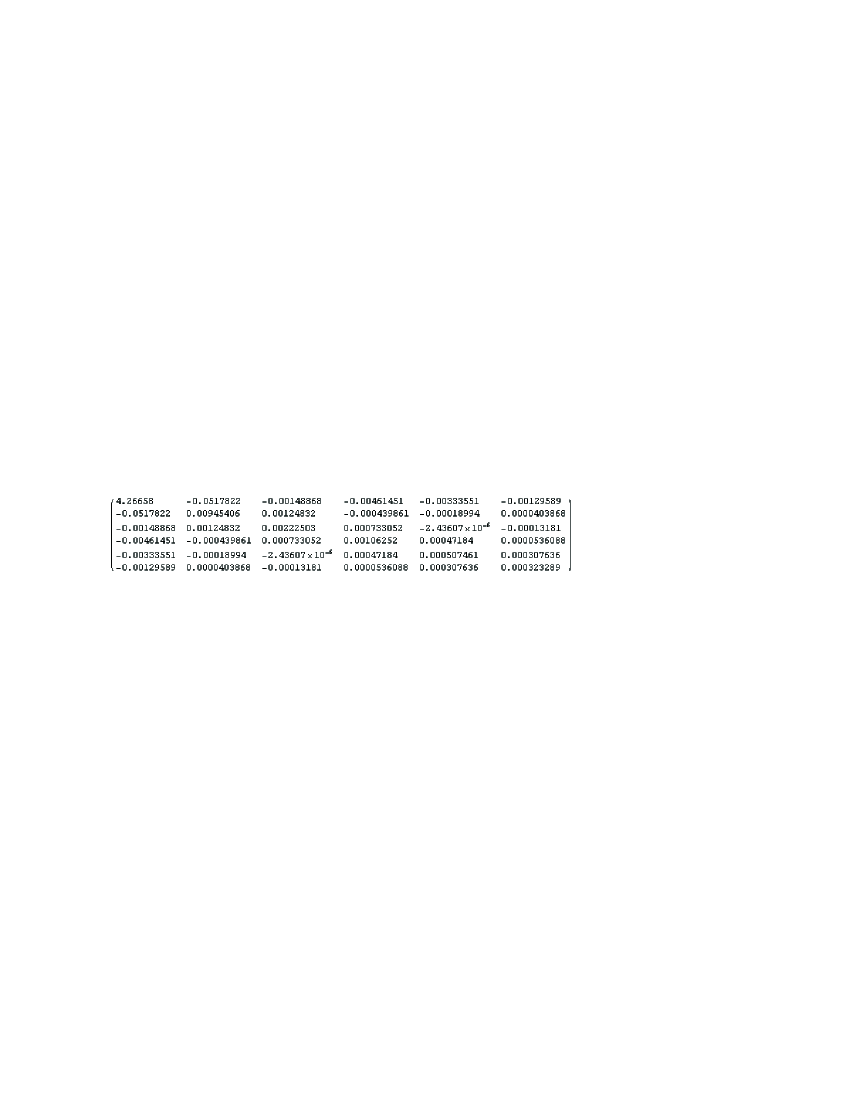
Figure 3: An example of the obtained covariance matrix $\bf{K}_{yy}$ for $N_{s}=6$ samples and $N_{w}=28$ wave functions

By solving numerically the eigenvalue problem for this covariance matrix we obtain the KL transformation matrix $\bf{\Phi}$ presented in figure 4, also only for 6 samples per wave function.

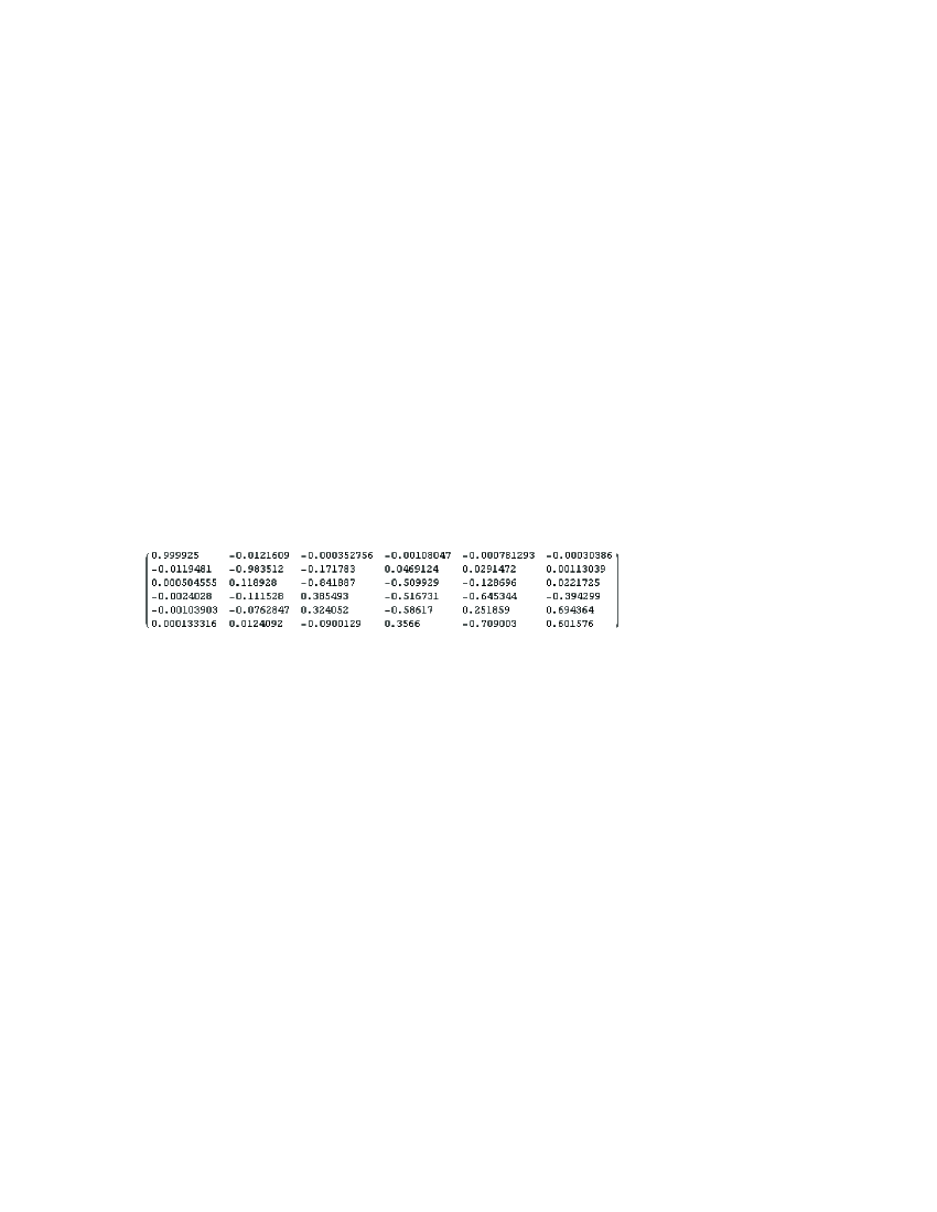
Figure 4: An example of the KL transform matrix $\bf{\Phi}$, for $N_{s}=6$ samples and $N_{w}=28$ wave functions. Each column contains the samples of a function $\bf{\Phi}_{i}$ of the optimal basis set

For a realistic calculation, we used $N_{s}=20$ equidistant samples and from the covariance matrix (not shown here) we obtained the eigenvalues listed in figure 5. The equidistant sampling method was chosen for simplicity of this exemplification but increasing errors are expected at the extremities of the interval due to the Runge phenomenon. Of course, in practice we recommend more appropriate sampling methods like those mentioned in chapter 3.

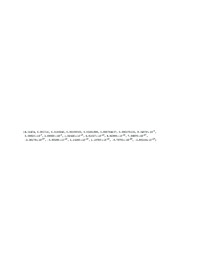
Figure 5: An example of the eigenvalues $\lambda_{i}$ obtained for $N_{s}=20$ samples and $N_{w}=28$ wave functions

One may see that the eigenvalues are indeed rapidly decreasing, confirming the possibility of reducing the dimension of the basis set, as it was anticipated in the previous subsection. It follows from the presented values that only 8-10 eigenvectors should be considered, the others corresponding to much smaller eigenvalues.

For solving the differential equations using spectral methods, one needs the derivatives of the basis function. Taking into account that these function are known in a small number of points (their samples) it is not effective to use a direct numerical differentiation. Instead, one may interpolate those samples for each of the basis functions and thus obtain an analytical expression, for example a polynomial. For the sake of simplicity, we used a Lagrange interpolation (but some other methods may be investigated for better results) and obtained the basis functions as exemplified in figure 6.

Figure 6: Some of the basis set functions obtained for $N_{s}=20$ samples and $N_{w}=28$ wave functions

Using these analytical form for the basis set, we checked the numerical solving of the radial differential equation 4.1 with the following parameters: $\ell=0,\;n=1,\;E_{n}=-0.5,\;N_{s}=8,\;a=0,\;b=7,\;y_{f}=10^{-4},\;\epsilon=10^{-10}$. We obtained a wave function as presented in figure 7, which is very close to the analytical one presented dashed in the same figure.

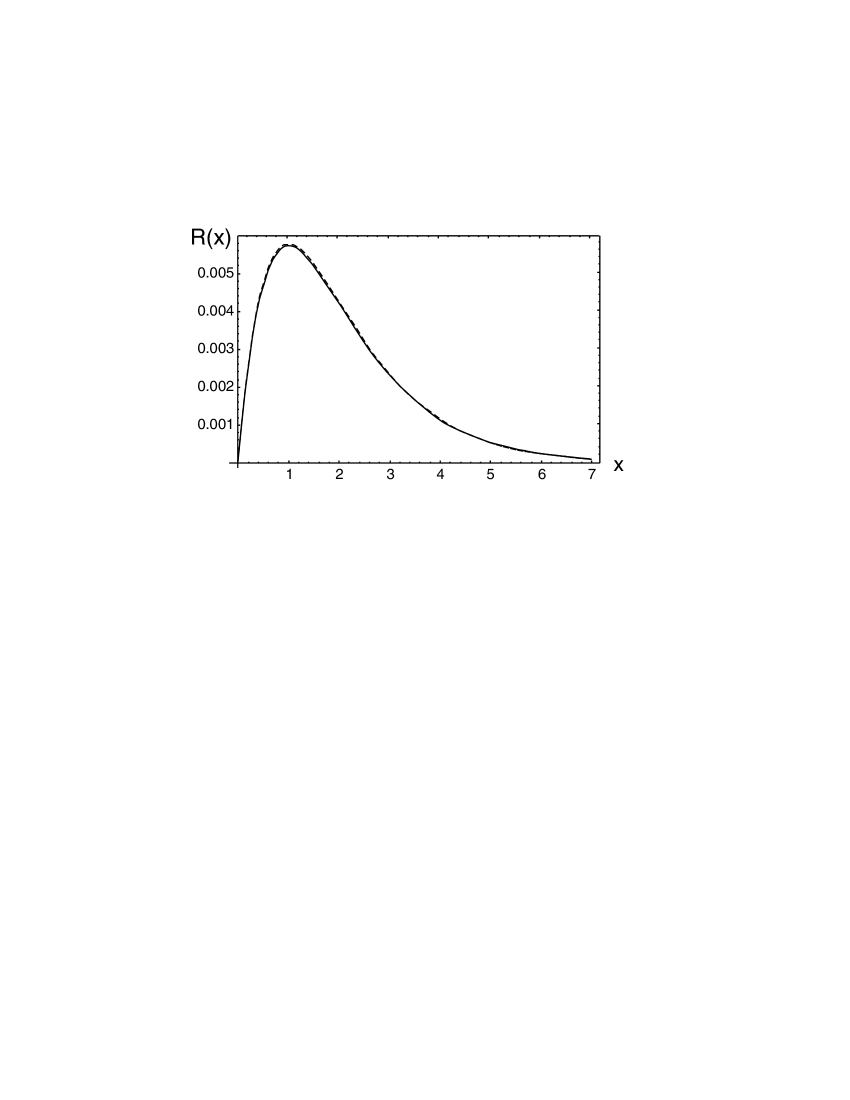
Figure 7: A comparison of the analytical solution (dashed) with the numerical one (continous) obtained for $N_{s}=20$ samples and $N_{w}=28$ wave functions

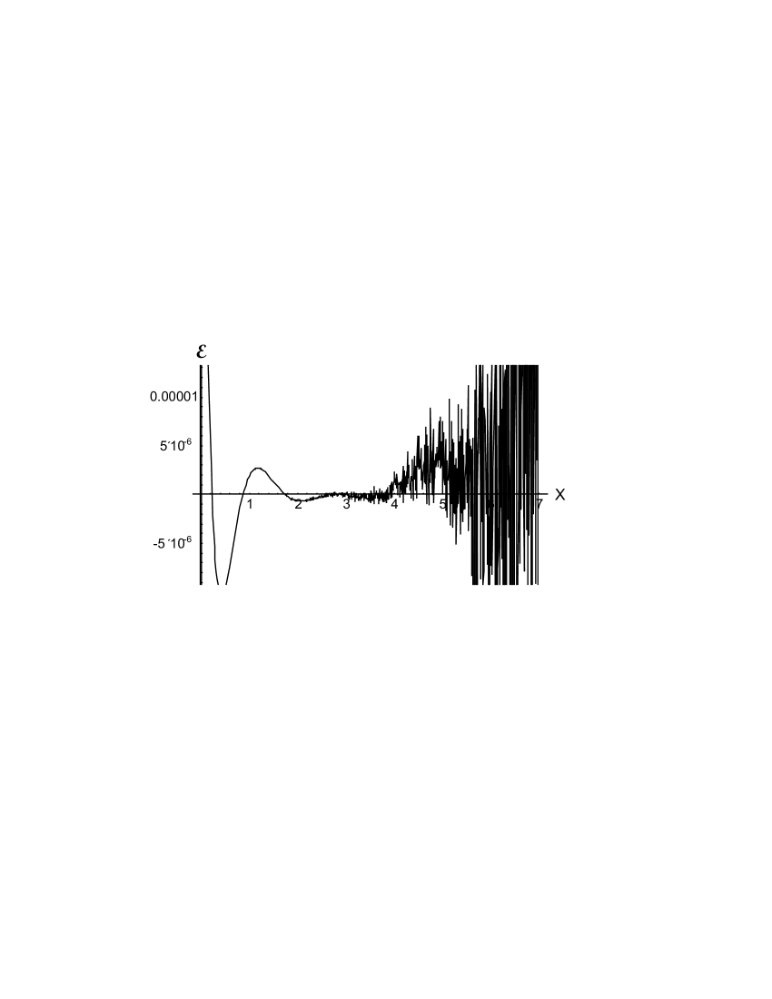
Figure 8: Difference between the two members of the radial equation obtained for $N_{s}=20$ samples and $N_{w}=28$ wave functions

The errors introduced by the interpolated basis set, obtained as the difference of the two members of the differential equation are presented in figure 8, where one may see the effect of the uniform sampling that we used for this example: the errors are highly increasing towards the boundaries. Also, the result of the bad conditioning of the system (3.2) may be noticed for high values of x both in figure 7 and figure 8. It is possible that this conditioning should be improved if proper sampling and interpolation techniques are used. Anyway, the result is very encouraging, taking into account that for other basis sets (for example gaussian), in similar conditions, clearly higher errors are displayed.

5 Conclusions

Although the above presented method is highly susceptible for improvements, the simple example presented for implementing the concept of the optimal basis set obtained using the covariance matrix over the set of typical wave functions gives satisfactory results. The most important feature of the method is the virtual increase in speed due to the theoretically smallest number of basis functions needed and their construction using the information contained in a big number of possible orbitals.

The price paid is the necessity to calculate and diagonalize the covariance matrix, but it is important to notice that it must be done only at the start of the iteration process and maybe in some intermediate steps. The assertion above is experimentally proved by the fact that in data processing an initial set of samples may be used for constructing covariance matrices adequate for other different situations.

Improvements of the presented example may be made in the sampling and interpolations processes and the principle may be also applied to other various spectral methods used by ab initio calculations.

References

References

- [1] W. Kohn and L.J. Sham, Phys. Rev, 140, A113 (1965)
- [2] J.C. Slater, Quantum Theory of Molecules and Solids, Vol. 4: The Self-Consistent Field for Molecules and Solids (McGraw-Hill, New
- [3] York, 1974) 4. A.D. Becke, Phys. Rev. A 38, 3098 (1988).
- [4] J. P. Perdew and Y. Wang Phys. Rev. B 45, 13244 - 13249 (1992)
- [5] J.P. Perdew, in Electronic Structure Theory of Solids, P. Ziesche and H. Eschrig, eds. (Akademie Verlag, Berlin, 1991); J.P. Perdew, J.A. Chevary, S.H. Vosko, K.A. Jackson, M.R. Pederson, D.J. Singh, and C. Fiolhais, Phys. Rev. B 46, 6671 (1992).
- [6] . S.H. Vosko,L. Wilk, and M. Nusair, Can. J. Phys. 58, 1200 (1980).
- [7] J.P. Perdew and A. Zunger, Phys. Rev. B 23, 5048 (1981).
- [8] C. Lee, W. Yang, and R.G. Parr, Phys. Rev. B 37, 785 (1988);
- [9] W.H. Press, B.P. Flannery, S.A. Teukolsky, and W.T. Vetterling, Numerical Recipes in C++, The art of scientific Computing. Cambridge University Press, 1999.
- [10] C. C. J. Roothaan, Reviews of ModernPhysics, 23, 69, (1951)
- [11] J. P. Boyd, Chebyshev and Fourier Spectral Methods, DOVER Publications, Inc. 2000
- [12] R.A. Friesner, J. Phys.Chem. 92, 3091 (1988).
- [13] Albert Messiah, Quantum Mechanics, John Wiley and Sons, 1966
- [14] K. Karhunen, Kari, Über lineare Methoden in der Wahrscheinlichkeitsrechnung, Ann. Acad. Sci. Fennicae. Ser. A. I. Math.-Phys., 1947, No. 37, 1–79
- [15] M.M. Loève, Probability Theory,Princeton, N.J.: VanNostrand, 1955
- [16] J.L. Lumley, Atmospheric turbulence and radio propagation, Moscow: Nauka, 1967,pp.166-178
- [17] C. L. Brooks, M. Karplus and B.M. Pettitt, Proteins: a Theoretical Perspective of Dynamics, Structure and Thermodynamics, New York: Wiley, 1988
- [18] H. Hotelling, Analisys of a complex of statistical variables into principal components, Journal of Educational Psychology, (1933) 24,pp. 417-441, 488-520
- [19] G.H. Golub, C.F. Van Loan, Matrix Computations, Oxford: North Oxford Academic, 1983