Counting Statistics in Multi-stable Systems

Abstract

Using a microscopic model for stochastic transport through a single quantum dot that is modified by the Coulomb interaction of environmental (weakly coupled) quantum dots, we derive generic properties of the full counting statistics for multi-stable Markovian transport systems. We study the temporal crossover from multi-modal to broad uni-modal distributions depending on the initial mixture, the long-term asymptotics and the divergence of the cumulants in the limit of a large number of transport branches. Our findings demonstrate that the counting statistics of a single resonant level may be used to probe background charge configurations.

I Introduction

The coexistence of several stationary states for a given set of parameters is typically referred to as the phenomenon of multi-stability. Multi-stable behavior is found in a wide variety of systems in different disciplines of science, as e.g. biology Angeli et al. (2004), chemistry Johánek et al. (2004), neuroscience Eagleman (2001), laser physics Arecchi et al. (1982), and semiconductor physics Galperin et al. (2008).

In transport systems, multi-stability is characterized by the existence of more than two distinct branches in the transport characteristics with hysteresis and switching in between. Some prototype examples for corresponding electronic systems are superlattices Kastrup et al. (1994), double-barrier resonant tunneling diodes Martin et al. (1994), and nano-electromechanical systems Wiersig et al. (2008). If the transport is entirely governed by stochasticity, e.g. as in single-electron transport Beenakker (1991), the current alone might not reveal the multi-stable character and other more sensitive tools are required. As has been shown for bistable systems Jordan and Sukhorukov (2004), the counting statistics Levitov and Lesovik (1993) may serve as such a tool. Recently, in Ref. Fricke et al. (2007) the measurement of a bi-modal distribution of quantum dot tunneling has indicated the interplay of fast and slow transport channels not visible in the current.

In this work, we present a generic approach to study Markovian transport systems with multi-stable behavior. Starting from a microscopic model for one transport channel with an environmental control system we derive a Master equation for Counting Statistics with an arbitrary number of transport branches. The resulting Liouville super-operator has a simple and scalable block-tridiagonal structure. Even though there exists a unique steady state, the counting statistics and higher-order cumulants display clear signatures of multi-stability such as multi-modal or broad distributions and diverging cumulants. We provide results for the temporal evolution and long-term asymptotics of the statistics and discuss the limit of a large number of coexisting current branches analytically. We emphasize that our approach is not restricted to electrons as transferred entities - in principle, stochastic multi-stable transport of any countable object can be studied by this means.

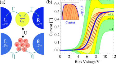
Figure 1: (Color online) (a) Scheme of the model. (b) Region of multi-stability: Current-voltage (Transport) characteristics for $N=7$ control dots; thin red curves: $N+1$ individual currents $I_{k}$ ($k=0,1,\dots,7$), thick blue line: average current $\langle I\rangle$ which is actually observed; Borders of colored regions: standard deviation $\pm c\sqrt{\left<\left<I^{2}\right>\right>}/2$ of the current which becomes divergent for $\eta\rightarrow 0$ in the multi-stability region. Inset: Broad uni-modal Distribution function $\log{(P)}/t$ vs. current for large times and $V^{*}=$7 (thick blue curve); distributions for individual currents $I_{k}$ (thin red curves). Parameters: $N=$7, $\epsilon_{d}$=3, $\beta$=3, $U$=0.15, $\eta$=0.001.

II Illustrative picture

A single transport channel (single resonant level, quantum dot) influenced by $k$ background charges distributed on a collection of $N$ sites will experience an effective shift of its charged energy state ($\epsilon_{d}\to\epsilon_{d}+kU$, where $U$ is the Coulomb repulsion). Attaching two reservoirs ($L$, $R$) held at different chemical potentials – see Fig. 1(a) – will now induce transport through the dot at rate $\Gamma$, which strongly depends on the number of background charges. Effectively, this leads to shifted currents in the transport channel

$$I_{k}=\frac{\Gamma}{2}\bigg{[}f_{L}(\epsilon_{d}+kU)-f_{R}(\epsilon_{d}+kU)\bigg{]}\,,$$ (1)

where $f_{L,R}(\omega)=\left[1+e^{+\beta(\omega\mp V/2)}\right]^{-1}$ denote the Fermi functions of the respective reservoir with bias voltage $V$, see Fig. 1(b). Coupling the background charges to different reservoirs $\bar{L}$, $\bar{R}$ with rate $\eta\ll\Gamma$ will cause slow random switching between the different transport channels $I_{k}$ (for two currents $k=0,1$ known as random telegraph noise Kogan (1998)). When the lead temperature is comparable to the Coulomb interaction $\beta^{-1}\approx U$, this gives rise to a pronounced region of multi-stability around $V^{*}\approx 2\epsilon_{d}+NU$ in the current-voltage characteristics, see Fig. 1(b). In this region, the second-order cumulant of the current $\left<\left<I^{2}\right>\right>$ diverges for $\eta\rightarrow 0$ as indicated. The inset shows the corresponding broad long-term distribution of currents at $V^{*}$ in comparison with the distributions of individual currents.

III Microscopic Model

III.1 Hamiltonian

We consider the total Hamiltonian

$$H = \epsilon_{d}d^{\dagger}d+\sum_{i=1}^{N}\epsilon_{i}d_{i}^{\dagger}d_{i}+\sum_{i=1}^{N}\sum_{j=i+1}^{N}U_{ij}d_{i}^{\dagger}d_{i}d_{j}^{\dagger}d_{j}$$ (2)

$$+\sum_{i=1}^{N}U_{i}d_{i}^{\dagger}d_{i}d^{\dagger}d+\sum_{ka}\omega_{ka}c_{ka}^{\dagger}c_{ka}$$

$$+\sum_{ka}t_{ka}\left[dc_{ka}^{\dagger}+c_{ka}d^{\dagger}\right]$$

$$+\sum_{ka}\sum_{i=1}^{N}\tau_{ka}^{i}\left[d_{i}c_{ka}^{\dagger}+c_{ka}d_{i}^{\dagger}\right]\,,$$

where $d$, $d_{i}$, and $c_{ka}$ annihilate electrons on the transport dot, the $i^{\rm th}$ control dot, and the mode $k$ on lead $a$ (with energy $\omega_{ka}$), respectively. In addition, we consider the symmetrized wide-band limit, where the transport dot tunneling rates $\Gamma\equiv 2\pi\sum_{k}{\left|t_{ka}\right|}^{2}\delta(\omega-\omega_{ka})$ and the control dot tunneling rates $\eta\equiv 2\pi\sum_{k}{\left|\tau_{ka}^{i}\right|}^{2}\delta(\omega-\omega_{ka})$ become independent of energy and lead. The parameters $U_{i}$ denote the Coulomb interaction between transport and control sites, whereas $U_{ij}$ represents repulsion between electrons within the control system. We assume that the spectrum of the system Hamiltonian is only near but not exactly degenerate $U_{i}\approx U$, $U_{ij}\approx U_{\rm c}$, and $\epsilon_{i}\approx 0$. These simplifications are not crucial for the occurrence of multi-stability, but rather allow for an analytic treatment in the following.

III.2 Liouvillian

We perform our analysis within the Born-Markov-secular approximation scheme which can be alternatively Schaller and Brandes (2008); Schaller et al. (2009) derived with a coarse graining method in the limit of infinitely large coarse graining times $\tau$. Provided the system energy spectrum is non-degenerate and the time scales are larger than the inverse minimum level splitting, the Liouvillian couples only the diagonals of the density matrix in the system energy eigenbasis with each other (see also Breuer and Petruccione (2002)). Since we are interested in observable effects of multi-stability in the current through the transport dot, we introduce a virtual detector in the right lead $R$ Schaller et al. (2009) via the replacement in the tunneling Hamiltonian $dc_{kR}^{\dagger}\to dc_{kR}^{\dagger}\otimes b^{\dagger}$ and $c_{kR}d^{\dagger}\to c_{kR}d^{\dagger}\otimes b$, where the detector operator $b^{\dagger}=\sum_{n}\left|n+1\right>\left<n\right|$ increases the detector outcome each time an electron is created in the right transport lead. Treating the tensor product of dot and detector Hilbert spaces as the system, we arrive at an $n$-resolved master equation of the form $\left<n\right|\dot{\rho}\left|n\right>\equiv\dot{\rho}^{(n)}=L_{0}\rho^{(n)}+L_{+}\rho^{(n-1)}+L_{-}\rho^{(n+1)}$, which couples different realizations of the dot density matrix – each valid for different particle numbers $n$ measured in the detector – with each other. This coupled system can be further reduced by Fourier-transformation $\rho(\chi,t)\equiv\sum_{n}\rho^{(n)}(t)e^{in\chi}$, where $\chi$ is the counting field, which leads to $\dot{\rho}(\chi,t)=\left(L_{0}+e^{+i\chi}L_{+}+e^{-i\chi}L_{-}\right)\rho(\chi,t)\equiv L(\chi)\rho(\chi,t)$.

Due to the permutational symmetry, it is convenient to denote the corresponding eigenstates for $N$ control sites by $\left|N,k,\ell;n_{\rm d}\right>$, where $\ell\in\left\{1,2,\ldots,\left(\begin{array}[]{c}N\\ k\end{array}\right)\right\}$ arbitrarily labels all the configurations with $0\leq k\leq N$ electrons distributed on the $N$ control sites, and $n_{\rm d}\in\{0,1\}$ denotes the occupation of the transport dot. When we trace out the configuration of the control dots for a given total number of control charges $k$ by defining the $2\times 2$ matrix $\rho_{k}(\chi,t)\equiv\sum_{\ell}\left<N,k,\ell\right|\rho(\chi,t)\left|N,k,\ell\right>$, the Liouvillian in this basis assumes for $0\leq k\leq N$ the form

$$\dot{\rho}_{k}(\chi,t) = \Gamma{\cal L}^{\rm dot}(\chi,\epsilon_{d}+kU)\rho_{k}(\chi,t)+\eta{\cal L}_{0k}^{\rm control}\rho_{k}(\chi,t)$$ (3)

$$+\eta(N-k+1){\cal J}_{k}^{\rm in}\rho_{k-1}(\chi,t)$$

$$+\eta(k+1){\cal J}_{k}^{\rm out}\rho_{k+1}(\chi,t)\,,$$

where the newly introduced super-operators are $2\times 2$ matrices, which obey ${\cal J}_{0}^{\rm in}\equiv\mbox{\boldmath$0$}$ and ${\cal J}_{N}^{\rm out}\equiv\mbox{\boldmath$0$}$ at the boundaries. This defines a $2(N+1)\times 2(N+1)$-dimensional Liouvillian super-operator $L(\chi)$ with a block-tridiagonal structure. The detailed structure of the reduced Liouvillian super-operators follows from a rigorous microscopic derivation, it may however also be understood from simple phenomenological reasoning:

(i) The multi-stable (fast) part has block-diagonal structure, where the $N+1$ block matrices correspond to the Liouvillian of a single resonant level – shifted by the Coulomb interaction with $k$ control charges

$${\cal L}^{\rm dot}(\chi,\omega) \equiv \left(\begin{array}[]{cc}-f_{L}(\omega)&f_{L}^{-}(\omega)\\ f_{L}(\omega)&-f_{L}^{-}(\omega)\end{array}\right)$$ (9)

$$+\left(\begin{array}[]{cc}-f_{R}(\omega)&e^{+i\chi}f_{R}^{-}(\omega)\\ e^{-i\chi}f_{R}(\omega)&-f_{R}^{-}(\omega)\end{array}\right)\,,$$

where $f_{a}^{-}(\omega)\equiv\left[1-f_{a}(\omega)\right]$. Evidently, when $\eta=0$, these matrices give rise to the multi-stable currents in Eq. (1). Since we have traced out the different control dot configurations, it also becomes obvious that the associated currents $I_{k}$ are actually $\left(\begin{array}[]{c}N\\ k\end{array}\right)$-fold degenerate. These degeneracies may be lifted (and thereby become observable) when the assumed symmetries of the Hamiltonian are absent.

(ii) The remaining part of the Liouvillian (which appears as slow when $\eta\ll\Gamma$) consists of the control system jump super-operators

$${\cal J}_{k}^{\rm in} \equiv \sum_{a\in\{\bar{L},\bar{R}\}}\left(\begin{array}[]{cc}f_{a}((k-1)U_{\rm c})&0\\ 0&f_{a}\left((k-1)U_{\rm c}+U\right)\end{array}\right)\,,$$ (12)

$${\cal J}_{k}^{\rm out} \equiv \sum_{a\in\{\bar{L},\bar{R}\}}\left(\begin{array}[]{cc}f_{a}^{-}(kU_{\rm c})&0\\ 0&f_{a}^{-}\left(kU_{\rm c}+U\right)\end{array}\right)\,,$$ (15)

which depend on the control system occupation number, and a trace-conserving part ${\cal L}_{0k}^{\rm control}\equiv-k{\cal J}_{k-1}^{\rm out}-(N-k){\cal J}_{k+1}^{\rm in}$. The scalar coefficients in Eq. (3) arise, since for any control configuration with $k-1$ charges there are $N-k+1$ different possibilities to obtain a control configuration with $k$ charges. Similarly, for a configuration with $k+1$ charges, each single charge leaving the control sector constitutes an equivalent jump channel Vogl et al. (2010). In addition, we note that the control jump super-operators (12) must assume diagonal form in the sequential tunneling regime for the basis chosen.

III.3 Transport observables

The probability for obtaining $n$ tunneled particles after time $t$ is given by $P_{n}(t)={\rm Tr}\left\{\rho^{(n)}(t)\right\}$. It follows that the moments of $P_{n}(t)$ may be directly obtained from the Fourier-transformed Liouvillian by suitable differentiation of the moment generating function (MGF)

$$M(\chi,t)={\rm\bf Tr}\left\{e^{L(\chi)t}\bar{\rho}\right\}$$ (16)

(where ${\rm\bf Tr}\left\{\left(\rho_{0},\ldots,\rho_{N}\right)\right\}\equiv\sum_{k=0}^{N}\rho_{k}$)) with respect to the counting field $\chi$. The initial density matrix $\bar{\rho}$ is typically chosen as the steady state $L(0)\bar{\rho}=0$, since one is usually interested in long-term cumulants. The matrix exponential is significantly harder to evaluate than the matrix inverse, such that we consider the Laplace transform

$$\tilde{M}(\chi,z)={\rm\bf Tr}\left\{\frac{1}{z\mbox{\boldmath$1$}-L(\chi)}\bar{\rho}\right\}$$ (17)

of the MGF instead.

For example, the moments of $P_{n}(t)$ are obtained via

$$\left<n^{k}\right>(t)=(-i\partial_{\chi})^{k}M(\chi,t).$$ (18)

The full distribution, however, is obtained by inverse Fourier transform

$$P_{n}(t)=\frac{1}{2\pi}\int\limits_{-\pi}^{+\pi}M(\chi,t)e^{-in\chi}d\chi.$$ (19)

IV Results

IV.1 Analytical steady state

When transport and control dots are coupled to leads with the same chemical potential ($f_{a}=f_{\bar{a}}$) and $\epsilon_{d}=0$ as well as $U=U_{\rm c}$, the steady state of Eq. (3) at $\chi=0$ is $\bar{\rho}=C_{N}\left(\bar{\rho}_{0},\dots\bar{\rho}_{N}\right)^{T}$, where the partial vectors read

$$\bar{\rho}_{k} = \left(\begin{array}[]{c}N\\ k\end{array}\right)\left[\prod_{\ell=0}^{k-1}p_{\ell}\right]\left[\prod_{\ell=k+1}^{N}2-p_{\ell}\right]\left(\begin{array}[]{c}2-p_{k}\\ p_{k}\end{array}\right)$$ (24)

with $p_{k}\equiv f_{L}(kU)+f_{R}(kU)$ and $C_{N}$ follows from normalization. The corresponding current $I={\rm Tr}\left\{L^{\prime}(0)\bar{\rho}\right\}$ is the weighted sum of partial currents $I_{k}$ (1). The current-voltage characteristic exhibits $2N$ steps for small temperatures $\beta\Delta\gg$1 ($\Delta\equiv NU$) which become smeared out for $\beta\Delta\lesssim$1 as shown in Fig. 2(a). Therefore, for sufficiently low temperatures we are able to probe the number $N$ just by a current measurement. At larger temperatures, however, this fails and the counting statistics will provide a proper tool for that purpose (see Fig. 3 and corresponding discussion). In the thermodynamic limit ($N\rightarrow\infty$, $U\rightarrow$0) such that the band-width $\Delta$ stays finite [spectrum becomes continuous as sketched in inset of Fig. 2(b)] the characteristic is linear for $\beta\Delta\gg$1 and $|V|<\Delta$ with Ohm’s resistance of $2\Delta/\,e\Gamma$ [compare Fig. 2(b)].

Figure 2: (Color online) Current-voltage characteristics for a nontrivial non-thermal stationary state (24). (a) for various temperatures $\beta\Delta$ and $N=$10; at small temperatures ($\beta\Delta\gg$1) the number of control dots $N$ can be probed in a current measurement, whereas at $\beta\Delta\lesssim$1 one has to make use of counting statistics at $t\lesssim\eta^{-1}$ (see Fig. 3). (b) for various $N$ and $\beta\Delta=$40; for $N\rightarrow\infty$, $U\rightarrow$0, $|V|<\Delta$ and $\beta\Delta\gg$1 the current becomes linear $I=\frac{e\Gamma}{2\Delta}V$ since transport takes place through a continuum with finite band-width $\Delta\equiv NU$ (as sketched in the inset).

IV.2 Full Counting Statistics

The model (2) shows very rich behavior. We, however, choose some limiting cases to illustrate the multistable properties in the following:

(i) In the infinite bias limit $f_{L}\to 1$ and $f_{R}\to 0$, the MGF coincides with that of a single resonant level, for which we obtain

$$P_{n\geq 0}(t) = \frac{e^{-\Gamma t}(\Gamma t)^{2n-1}}{2(2n+1)!}\times$$

$$\times\left[2n(2n+1)+(4n+2)\Gamma t+(\Gamma t)^{2}\right]$$

and $P_{n<0}(t)=0$, such that the counting statistics will not reveal any multi-stable properties [compare Fig. 1(b) for large $V$].

(ii) When the control leads are at infinite bias, i.e. $f_{\bar{L}}(\omega)\to 1$ and $f_{\bar{R}}(\omega)\to 0$ such that ${\cal J}_{k}^{\rm in}={\cal J}_{k}^{\rm out}=\mbox{\boldmath$1$}$, and the transport leads are at high bias ($f_{R}(\omega)\approx 0$), one may for sufficiently low temperatures have $f_{L}(\epsilon_{d}+(k<\bar{k})U)=1$ and $f_{L}(\epsilon_{d}+(k\geq\bar{k})U)=0$ for some $\bar{k}\in\{1,\ldots,N\}$, which leads to only two different currents (bistable case). The detailed form of the Liouvillian and its counting statistics then depends on $N$ and $\bar{k}$, but the whole class of bistable models is amenable to analytic investigations. In the simplest case of $\bar{k}=N=1$, we have for $\eta=0$ a bimodal distribution: Half of the distribution follows the evolution of a single resonant level (IV.2), and the other half remains localized at $n=0$ for all times. The situation becomes non-trivial for finite $\eta$, which is reflected in the recursive relation for the Laplace transform $\tilde{P}_{n+1}(z)={\cal F}(z)\tilde{P}_{n}(z)$ for $n\geq 2$, where ${\cal F}(z)$ has four different first order poles, such that – unlike Eq. (IV.2) – the complexity of $P_{n}(t)$ will increase with $n$.

(iii) Under the same (infinite and high bias, respectively) assumptions we may adjust bias voltage and temperature such that we can distribute the left-associated Fermi-functions in an approximately equidistant manner between zero and one (such as e.g. $f_{L}(\epsilon_{d})=1$, $f_{L}(\epsilon_{d}+U)=2/3$, $f_{L}(\epsilon_{d}+2U)=1/3$, and $f_{L}(\epsilon_{d}+3U)=0$ for $N=3$), we can analytically extract the current $\left<\left<\dot{n}^{1}(t)\right>\right>=\frac{\Gamma}{4}$ and the long-term scaling of the next higher cumulants (for $N\neq 0$) of $P_{n}(t)$

$$\left<\left<n^{2}(t)\right>\right> \to \frac{\Gamma\left(3N\eta^{2}+3N\eta\Gamma+\Gamma^{2}\right)}{16N\eta\left(\Gamma+\eta\right)}t\,,$$

$$\left<\left<n^{3}(t)\right>\right> \to \frac{\Gamma}{64}\left[7+\frac{3\Gamma^{2}\left(2\Gamma+3\eta\right)}{\eta N\left(\Gamma+\eta\right)^{2}}\right]t\,.$$ (27)

These expressions demonstrate that the higher cumulants diverge for small $\eta$ in the long time limit. In the limit of an infinite number of multi-stable channels ($N\to\infty$) however, this divergence is overshadowed by the exponentially large degeneracy of intermediate currents: If the control jump matrices in Eq. (3) did not scale with $N$, the divergence of all higher than second cumulants would persist also in the limit $N\to\infty$.

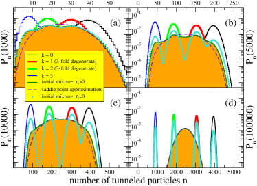
Figure 3: (Color online) Probability distribution $P_{n}(t)$ for the number of tunneled particles $n$ at different times $t$ (orange region). For increasing times [(a) $\rightarrow$ (d)] the average of the distribution moves linearly towards larger $n$. It proceeds a crossover from multi-modal to unimodal with a transition time of $\eta^{-1}$ and becomes (nearly) a broad Gaussian for $t\gg\eta^{-1}$ (d). For $\eta=0$ even the long-term distribution depends on the initial mixture (symbols) here chosen as analytic continuation of $\bar{\rho}$ to $\eta=0$, which reflects in the different peak weights. For comparison: Distributions $P_{n}^{(k)}(t)$ for individual currents $I_{k}$ (blue, bold green, bold red, and black curves in the background). The saddle-point approximation (dashed lines) only captures the long-term behavior $t\gg\eta^{-1}$. Parameters: $N=3$, $\epsilon_{d}=1$, $\Gamma=0.1$, $\eta=0.0001$, $U=1$, $\beta=1$, $V=V^{*}=5$, $\bar{V}\to\infty$.

(iv) Without these assumptions, we can still numerically perform both the inverse Laplace transform of $\tilde{M}(\chi,z)$ and a Fourier integral to obtain $P_{n}(t)$, which is typically evaluated using the saddle-point approximation Schaller et al. (2009) [compare also inset of Fig. 1(b)]. The result in the multi-stable bias regime of interest is shown for different times in Fig. 3. Choosing $\bar{\rho}$ for $\eta>0$ as initial mixture, the statistics is multi-modal with $N+1$ maxima for $t\lesssim\eta^{-1}$ [Figs. 3(a) and (b)]. In contrast, the statistics becomes uni-modal for $t\gtrsim\eta^{-1}$ [Figs. 3(c) and (d)]. In the long-term limit, the distribution for $\eta>0$ evolves essentially into a broad Gaussian (d). This is a general property of systems with cumulants linearly evolving in time. In contrast, when $\eta=0$, $P_{n}(t)$ will depend on the initial configuration for all times. For example, when one initializes in one of the subspaces $k=0,\dots,N$, one will observe the distributions $P_{n}^{(k)}(t)$ for the individual currents $I_{k}$ (curves in the background in Fig. 3). Starting in a statistical mixture for $\eta=0$ yields a multi-modal distribution even in the long-term limit (symbols in Fig. 3) and leads to a divergence of all higher-order cumulants.

IV.3 Experimental parameters

For the observation of a multi-modal distribution (e.g. bi-modal in Ref. Fricke et al. (2007)) the measurement time must lie between $\Gamma^{-1}$ and $\eta^{-1}$. The rates in Ref. Fricke et al. (2007) are of the order of $\Gamma\approx 1\rm kHz$ and $\eta\approx 1\rm Hz$, respectively, such that the time of measurement can be estimated between $1$ ms and $1$ s. For a distance of a hundred $\rm nm$ between transport and control system, the Coulomb interaction strength in GaAs can be estimated to $U\approx 1.2\rm meV$. Provided the picture of a single transport level is still valid (i.e., for a significantly larger on-site Coulomb interaction energy), pronounced multi-stability should be observable around temperatures of $T\approx 14\rm K$. Larger distances or screened Coulomb interactions would lead to lower temperatures.

V Conclusions and Outlook

We have studied stochastic multi-stable transport in terms of an $n$-resolved Master equation with a simple and scalable block-tridiagonal Liouville super-operator (3). Multi-stability can be revealed by the full counting statistics even when the first moments are insensitive: For measurement times smaller than the switching rate between the distinct transport channels the distributions are multi-modal when the initial state is a mixture of the multiple steady states for $\eta=0$ (this is the case for $\bar{\rho}$ for finite $\eta$). This enables direct access to the number of decoupled non-degenerate subspaces. For longer times or degenerate subspaces this is not possible. However, unusually large higher-order cumulants may point towards intrinsic multi-stability. In case of sufficiently low temperatures multi-stable distributions may become effectively bi-stable.

However, if the initial mixture is strongly localized within one of the multiple subspaces (this would be a consequence of a projective measurement), a particle-number measurement would result in the associated current with high probability and all other currents with low probabilities. Consequently, a sequence of repeated measurements would yield the switching dynamics observed for single-charge counting detectors Gustavsson et al. (2006); Fricke et al. (2007); Flindt et al. (2009).

We finally remark that multi-stable behavior can also emerge due to the effect of coherences Schaller et al. (2009).