Stringent constraints on the scalar $K\pi$ form factor from analyticity, unitarity and low-energy theorems

Abstract

We investigate the scalar $K\pi$ form factor at low energies by the method of unitarity bounds adapted so as to include information on the phase and modulus along the elastic region of the unitarity cut. Using at input the values of the form factor at $t=0$ and the Callan-Treiman point, we obtain stringent constraints on the slope and curvature parameters of the Taylor expansion at the origin. Also, we predict a quite narrow range for the higher order ChPT corrections at the second Callan-Treiman point.

1 Introduction

The low energy properties of the $K\pi$ form factors are of great interest both experimentally and theoretically. In particular, a precise knowledge of the slope and curvature parameters at $t=0$ would serve to improve the experimental analysis of $K_{l3}$ decays, confirm the predictions of chiral perturbation theory (ChPT) and provide benchmarks for future lattice determination of these quantities.

In the present paper we consider the scalar $K\pi$ form factor, expanded as

$$f_{0}(t)=f_{0}(0)\left(1+\lambda_{0}^{\prime}\,\frac{t}{M_{\pi}^{2}}+\frac{1}{2}\lambda_{0}^{\prime\prime}\,\frac{t^{2}}{M_{\pi}^{4}}+\cdots\right),$$ (1)

in the physical region of $K_{l3}$ decay. The dimensionless parameters $\lambda_{0}^{\prime}$ and $\lambda_{0}^{\prime\prime}$ are related by $\lambda_{0}^{\prime}=M_{\pi}^{2}\langle r^{2}_{\pi\text{K}}\rangle/6$ and $\lambda_{0}^{\prime\prime}=2M_{\pi}^{4}c$ to the radius $\langle r^{2}_{\pi\text{K}}\rangle$ and curvature $c$ used alternatively in the literature.

The $K\pi$ form factors have been calculated at low energies in ChPT GaLe19851 ; GaLe19852 ; BiTa and on the lattice (for recent reviews see LL2009 ; HL2009 ). At $t=0$, the present value $f_{+}(0)=0.962\pm 0.004$ LL2009 shows that the corrections to the Ademollo-Gatto theorem are quite small. Other low energy theorems frequently used are CallanTreiman -Oehme

$$f_{0}(\Delta_{K\pi})=\frac{F_{K}}{F_{\pi}}+\Delta_{CT},\quad f_{0}(\bar{\Delta}_{K\pi})=\frac{F_{\pi}}{F_{K}}+\bar{\Delta}_{CT},\quad$$ (2)

where $\Delta_{K\pi}=M^{2}_{K}-M^{2}_{\pi}$ and $\bar{\Delta}_{K\pi}=-\Delta_{K\pi}$ are the first and second Callan-Treiman points, respectively. The lowest order values are known from $F_{K}/F_{\pi}=1.193\pm 0.006$ LL2009 , and the corrections calculated to one loop are $\Delta_{CT}=-3.1\times 10^{-3}$ and $\bar{\Delta}_{CT}=0.03$ GaLe19852 . The higher order corrections appear to be negligible at the first point KaNe , but are expected to be quite large at the second one.

Analyticity and unitarity represent a powerful tool for obtaining information on the $K\pi$ form factors. Several comprehensive dispersive analyses were performed recently, using either the coupled channels Muskhelishvili - Omnès equations Jaminscalar2002 ; Bachirscalar2009 , or a single channel Omnès representation BePa .

Alternatively, the method of unitarity bounds, proposed a long time ago in Okubo ; SiRa , and applied since then to various electromagnetic and weak form factors, exploits the fact that a bound on an integral of the modulus squared of the form factor along the unitarity cut is sometimes known from independent sources. Standard mathematical techniques then allow one to correlate the values of the form factor at different points or to control the truncation error of power expansions used in fitting the data BoCaLe .

For the $K\pi$ system the method was applied in BoMaRa and more recently in BC ; AbAn . In Ref. BC the method was extended by including the phase of the scalar form factor along the elastic part of the cut, known from the elastic $K\pi$ scattering by Watson’s theorem, while in AbAn information on the form factor at the second Calln-Treiman point was included for the first time in the frame of the standard bounds.

In the present work we revisit the issue of bounds on the expansion coefficients (1) by applying a more sophisticated version of the unitarity bounds proposed in Caprini2000 . The method uses the fact that the knowledge of the phase allows one to remove the elastic cut and define a function with a larger analyticity domain. To be optimal, the method requires also some information on the modulus of the form factor in the elastic region. In BC , where the phase constraint was treated using Lagrange multipliers, this stronger property of the phase was not exploited, since no experimental information on the modulus was available at that time.

More recently, the precise measurements of the $\tau\to K\pi\nu_{\tau}$ spectral function by Belle collaboration Belle provided also a first direct experimental determination of the modulus of the $K\pi$ form factors below a certain energy. The modulus is available also from the dispersive analyses Jaminscalar2002 ; Bachirscalar2009 . This justifies the application of the method proposed in Caprini2000 . Our work extends the analysis made in AbAn by including information on the phase and modulus of the form factor on a part of the cut, which leads to a considerable improvement of the bounds. In the next section we describe briefly the method for the scalar form factor, and in section 4 we present the results. A more detailed analysis, including a discussion of the experimental implications and of the vector form factor, will be presented in AACIR2 .

2 Standard and new unitarity bounds

The method makes use of the following mathematical result: let $g(z)$ be a function analytic in the unit disk $|z|<1$ of the complex $z$-plane, which satisfies the inequality:

$$\frac{1}{2\pi}\int^{2\pi}_{0}d\theta|g(\exp(i\theta))|^{2}\leq I,$$ (3)

where $I$ is a positive number. Then, if

$$g(z)=g_{0}+g_{1}z+g_{2}z^{2}+\cdots$$ (4)

is the Taylor expansion of $g(z)$ at $z=0$, and $g(z_{1})$, $g(z_{2})$ denote the values of $g$ at two points inside the analyticity domain, $|z_{1}|<1,~{}|z_{2}|<1$ (for simplicity we assume that $z_{1}$ and $z_{2}$ are real), the following determinantal inequality holds:

$$\left|\begin{array}[]{c c c c c c}I&g_{0}&g_{1}&g_{2}&g(z_{1})&g(z_{2})\\ g_{0}&1&0&0&1&1\\ g_{1}&0&1&0&z_{1}&z_{2}\\ g_{2}&0&0&1&z_{1}^{2}&z_{2}^{2}\\ g(z_{1})&1&z_{1}&z_{1}^{2}&(1-z_{1}^{2})^{-1}&(1-z_{1}z_{2})^{-1}\\ g(z_{2})&1&z_{2}&z_{2}^{2}&(1-z_{2}z_{1})^{-1}&(1-z_{2}^{2})^{-1}\\ \end{array}\right|\geq 0.$$ (5)

Moreover, all the principal minors of the above matrix should be nonnegative. For the proof see Refs. Okubo ; SiRa ; BoMaRa .

To obtain this formulation for the scalar $K\pi$ form factor, one starts from a dispersion relation for the scalar polarization function of the $s$ and $u$ quarks BoMaRa ; BC ; AbAn ; Hill :

$$\chi_{{}_{0}}(Q^{2})\equiv\frac{\partial}{\partial q^{2}}\left[q^{2}\Pi_{0}\right]=\frac{1}{\pi}\int_{t_{+}}^{\infty}\!dt\,\frac{t{\rm Im}\Pi_{0}(t)}{(t+Q^{2})^{2}}\,,$$ (6)

where unitarity implies the inequality:

$${\rm Im}\Pi_{0}(t)\geq\frac{3}{2}\frac{t_{+}t_{-}}{16\pi}\frac{[(t-t_{+})(t-t_{-})]^{1/2}}{t^{3}}|f_{0}(t)|^{2}\,,$$ (7)

with $t_{\pm}=(M_{K}\pm M_{\pi})^{2}$. We use here the notations from Hill , where $\Pi_{0}$ is defined as the longitudinal part of the correlator of two vector currents. As in BC , $\Pi_{0}$ can be identified with $(\Psi(t)-\Psi(0))/t^{2}$, where $\Psi$ is the correlator of the divergence of the vector current.

The quantity $\chi_{{}_{0}}(Q^{2})$ in (6) can be reliably calculated by pQCD when $Q\gg\Lambda_{\rm QCD}$. At present, calculations available up to the order $\alpha_{s}^{4}$ GeBr -BaCh give:

$$\chi_{0}(Q^{2}) = \frac{3(m_{s}-m_{u})^{2}}{8\pi^{2}Q^{2}}\,\big{[}1+1.80\alpha_{s}$$ (8)

$$+ 4.65\alpha_{s}^{2}+15.0\alpha_{s}^{3}+57.4\alpha_{s}^{4}\dots\big{]},$$

where the running quark masses and the strong coupling $\alpha_{s}$ are evaluated at the scale $Q^{2}$ in $\overline{MS}$ scheme.

Taking into account the fact that $f_{0}(t)$ is analytic everywhere in the complex $t$-plane except for the branch cut running from $t_{+}$ to $\infty$, the relations (6)-(8) can be expressed in the canonical form (3) if one defines the variable

$$z(t)=\frac{\sqrt{t_{+}}-\sqrt{t_{+}-t}}{\sqrt{t_{+}}+\sqrt{t_{+}-t}},$$ (9)

which maps the $t$ plane cut from $t_{+}$ to $\infty$ onto the unit disk $|z|<1$, such that $z(0)=0$, and the function

$$g(z)=f_{0}(t(z))\,w(z),$$ (10)

where $t(z)$ is the inverse of (9) and $w(z)$ is the outer function BoMaRa - AbAn :

$$w(z) = \frac{\sqrt{3}}{32\sqrt{\pi}}\,\frac{M_{K}-M_{\pi}}{M_{K}+M_{\pi}}\,(1-z)\,(1+z)^{3/2}$$ (11)

$$\times\,\frac{(1+z(-Q^{2}))^{2}}{(1-z\,z(-Q^{2}))^{2}}\frac{(1-z\,z(t_{-}))^{1/2}}{(1+z(t_{-}))^{1/2}}.$$

Then (3) is satisfied, with

$$I=\chi_{0}(Q^{2}).$$ (12)

It may be noted that $z$ is an independent variable in the outer function, whereas $z(-Q^{2})$ etc., are defined via the conformal variable eq.(9).

We use now the fact that, below the inelastic threshold $t_{\rm in}$, the phase of the form factor $f_{0}(t)$ is known from Watson’s theorem and the $I=1/2$ $S$-wave of elastic $K\pi$ scattering. Then one can define the Omnès function

$${\cal{O}}(t)=\exp\left(\displaystyle\frac{t}{\pi}\int^{\infty}_{t_{+}}dt^{\prime}\displaystyle\frac{\delta(t^{\prime})}{t^{\prime}(t^{\prime}-t)}\right),$$ (13)

where $\delta(t)$ is the phase of the form factor known for $t\leq t_{\rm in}$, and is an arbitrary function, sufficiently smooth (i.e. Lipschitz continuous) for $t>t_{\rm in}$. It can be shown AACIR2 that the results are independent of the function $\delta(t)$ for $t>t_{\rm in}$.

Since the Omnès function ${\cal{O}}(t)$ fully accounts for the second Riemann sheet of the form factor, the function $h(t)$, defined by

$$f_{0}(t)=h(t)\,{\cal{O}}(t),$$ (14)

is real analytic in the $t$-plane with a cut only for $t\geq t_{\rm in}$. Then, the relations (6)-(8) and (14) can be expressed in the canonical form (3), by defining the new variable Caprini2000

$$z(t)=\displaystyle\frac{\sqrt{t_{\rm in}}-\sqrt{t_{\rm in}-t}}{\sqrt{t_{\rm in}}+\sqrt{t_{\rm in}-t}},$$ (15)

which maps the $t$-plane cut for $t>t_{\rm in}$ onto the unit disk $|z|<1$ of the $z$-plane, such that $z(0)=0$, and define the function Caprini2000

$$g(z)=f_{0}(t(z))\,w(z)\,\omega(z)\,[{\cal{O}}(t(z))]^{-1},$$ (16)

where $t(z)$ is now the inverse of (15). The new outer function $w(z)$ is defined as

$$w(z) = \frac{\sqrt{3}(M_{K}^{2}-M_{\pi}^{2})}{16\sqrt{2\pi}t_{\rm in}}\frac{\sqrt{1-z}\,(1+z)^{3/2}(1+z(-Q^{2}))^{2}}{(1-z\,z(-Q^{2}))^{2}}$$ (17)

$$\times\,\frac{(1-z\,z(t_{+}))^{1/2}\,(1-z\,z(t_{-}))^{1/2}}{(1+z(t_{+}))^{1/2}\,(1+z(t_{-}))^{1/2}},$$

and

$$\omega(z)=\exp\left(\displaystyle\frac{\sqrt{t_{\rm in}-t(z)}}{\pi}\int^{\infty}_{t_{\rm in}}dt^{\prime}\displaystyle\frac{\ln|{\cal{O}}(t^{\prime})|}{\sqrt{t^{\prime}-t_{\rm in}}(t^{\prime}-t(z))}\right).$$ (18)

Then (3) is satisfied, where $I$ is defined as

$$I=\chi_{0}(Q^{2})-\frac{3}{2}\frac{t_{+}t_{-}}{16\pi^{2}}\int_{t_{+}}^{t_{\rm in}}\!dt\,\frac{[(t-t_{+})(t-t_{-})]^{1/2}|f_{0}(t)|^{2}}{t^{2}(t+Q^{2})^{2}}\,,$$ (19)

and is calculable if the modulus $|f_{0}(t)|$ is known at low energies, below $t_{\rm in}$. Thus, we can use the inequality (5) and the nonnegativity of the leading minors to obtain bounds on the parameters of the expansion (1). The Taylor coefficients in (4) are defined uniquely in terms of these parameters by (10) or (16). We further choose $z_{1}=z(\Delta_{K\pi})$ and $z_{2}=z(\bar{\Delta}_{K\pi})$, where $z$ is defined by (9) or (15), and express $g(z_{j})$ in terms of the values in (2), by using either (10) or (16).

In our analysis we take as inputs the values of the form factor at $t=0$ and $t=\Delta_{K\pi}$, the phase below $t_{\rm in}$ and the integral over the modulus required in (19). Then the constraints resulting from (5) restrict the coefficients $\lambda_{0}^{\prime}$, $\lambda_{0}^{\prime\prime}$ and the value of $f_{0}(t)$ at the second Callan-Treiman point $\bar{\Delta}_{K\pi}$.

3 Input

We work in the isospin limit, adopting the convention that $M_{K}$ and $M_{\pi}$ are the masses of the charged mesons. The inputs provided by the low energy theorems was discussed in the Introduction.

For choosing $t_{\rm in}$, we recall that the first inelastic threshold for the scalar form factor is set by the $K\eta$ state, which suggests to take $t_{\rm in}=1\,\mbox{GeV}^{2}$ as in BC . However, this channel has a weak effect, the elastic region extending practically up to the $K\eta^{\prime}$ threshold, which justifies the choice $t_{\rm in}=(1.4\,\mbox{GeV})^{2}$. In our analysis we shall use for illustration these two values of $t_{\rm in}$.

Below $t_{\rm in}$ the function $\delta(t)$ entering (13) is the phase of the $S$-wave of $I=1/2$ of the elastic $K\pi$ scattering Jaminscalar2006 ; Bachirscalar2009 . In our calculations we use as default the phase from Bachirscalar2009 . Above $t_{\rm in}$ we assume $\delta(t)$ as a smooth function approaching $\pi$ at high energies. We checked numerically that the bounds are independent of the choice of $\delta(t)$ for $t>t_{\rm in}$.

To estimate the integral appearing in (19), we first used the parametrization of $|f_{0}(t)|$ in terms of the resonances $\kappa$ and $K_{0}^{*}(1430)$, proposed by Belle collaboration Belle . Using as input the solution 1 in Table 4 and Eq. (7) of Belle , the integral has the value $66.08\times 10^{-6}$ for $t_{\rm in}=1\,\mbox{GeV}^{2}$, and $184.89\times 10^{-6}$ for $t_{\rm in}=(1.4\,\mbox{GeV})^{2}$. Although the parametrization used in Belle does not have good analytic properties, this fact is not relevant for our analysis: all that we need is a numerical estimate of the integral in (19). The analyticity of the form factor is implemented rigorously in our approach, for every numerical input.

Aternatively, using the modulus available from the dispersive analyses Jaminscalar2006 or Bachirscalar2009 , the low energy integral in (19) is $40.05\times 10^{-6}$ or $37.01\times 10^{-6}$, respectively, for $t_{\rm in}=1\,\mbox{GeV}^{2}$, and $89.31\times 10^{-6}$ or $81.26\times 10^{-6}$ for $t_{\rm in}=(1.4\,\mbox{GeV})^{2}$.

Finally, we take $Q^{2}=4\,\text{GeV}^{2}$ as in BC ; Hill , and obtain $\chi_{0}=(253\pm 68)\times 10^{-6}$, using in (8) $m_{s}(2\,\text{GeV})=98\pm 10\,\text{MeV},m_{u}(2\,\text{GeV})=3\pm 1\,\text{MeV}$ LL2009 and $\alpha_{s}(2\,\text{GeV})=0.308\pm 0.014$, which results from the recent average $\alpha_{s}(m_{\tau})=0.330\pm 0.014$ JaminBeneke ; Davier ; Bethke ; CaFi2009 . The error of $\chi_{0}$ includes also a contribution of 15%, of the order of magnitude of the last term in (8), to account for the truncation of the expansion.

4 Results

In order to illustrate the effect of the additional information on the phase and modulus, we compare in Fig. 1 the allowed domains in the plane $(\lambda_{0}^{\prime},\,\lambda_{0}^{\prime\prime})$, obtained with the standard and the new bounds, using only the constraint at $t=0$ (this case is obtained from (5) by removing the lines and columns that contain $g(z_{1})$ and $g(z_{2})$). The large ellipse is obtained with the standard bounds, (9)-(12), the small ones represent the new bounds, calculated with (15)-(19) for two values of $t_{\rm in}$. For $f_{0}(0)$ we took the central value 0.962. The left panel is obtained with the integral in (12) calculated with the modulus from Belle , for the right one we used the modulus from Jaminscalar2006 .

The inner ellipses are slightly smaller in the left panel than in the right one, because in the latter case the integral in (19) is smaller and $I$ is larger (it is easy to see that a larger value of $I$ leads to an ellipse of a larger size). Moreover, in the right panel the small ellipses are not contained entirely inside the large one, which means that among the functions satisfying the constraints (15)-(19) there are some that violate the original bounds (9)-(12). However, this does not mean that the conditions are inconsistent, since the ellipses have a nonzero intersection, which represents the allowed domain in this case.

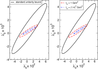
Figure 1: Allowed regions for the slope and curvature from the standard and the new bounds with the constraint at $t=0$. Left: modulus from Belle ; Right: modulus from Jaminscalar2006 .

The effect of the low-energy theorems (2) is illustrated in Fig. 2, which shows the improved bounds (15)-(19) calculated with the modulus from Belle for $t_{\rm in}=1\,\,\text{GeV}^{2}$. The large ellipse is obtained using the constraints at $t=0$ and $t=\Delta_{K\pi}$, the tiny ellipses result from the constraints at $t=0$, $\Delta_{K\pi}$ and $\bar{\Delta}_{K\pi}$, for the central values of $f_{0}(0)$ and $f_{0}(\Delta_{K\pi})$ and several values of the correction $\bar{\Delta}_{CT}$. The strong constraining power of the simultaneous constraints at $\Delta_{K\pi}$ and $\bar{\Delta}_{K\pi}$ was noted in AbAn . However, the bounds derived now are much stronger than those in AbAn , due to the additional information on the phase and modulus on the cut.

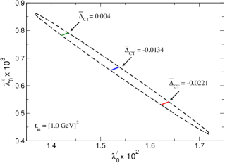
Figure 2: Large ellipse: new bounds obtained with $t_{\rm in}=1\,\,\text{GeV}^{2}$ and the values at $t=0$ and $\Delta_{K\pi}$; small ellipses: new bounds for $t_{\rm in}=1\,\,\text{GeV}^{2}$ and simultaneous constraints at $t=0$, $\Delta_{K\pi}$ and $\bar{\Delta}_{K\pi}$, for several values of $\bar{\Delta}_{CT}$.

The small ellipses exist only for $\bar{\Delta}_{CT}$ inside a rather narrow interval, whose end points lead to inner ellipses of zero size in Fig. 2. Actually, this range results directly from the inequality (5): by keeping only the lines and columns involving $g_{0}$, $g(z_{1})$ and $g(z_{2})$ and using the central values at $t=0$ and $\Delta_{K\pi}$, we obtain $-0.046\leq\bar{\Delta}_{CT}\leq 0.014$.

We recall that the current ChPT prediction is $-0.057<\bar{\Delta}_{CT}<0.089$ (cf. Eq. (4.9) of BePa adapted to our input $F_{K}/F_{\pi}$). As this interval is larger than the range derived above, we conclude that, at present, one can not further restrict the domain for the slope and curvature using the low-energy theorem at the second Callan-Treiman point: by varying $\bar{\Delta}_{CT}$ inside its currently known range we obtain the union of the tiny ellipses in Fig. 2, which covers the large ellipse obtained using only the value at $\Delta_{K\pi}$.

In Fig. 3 we show the allowed domains for the slope and curvature obtained with the constraints at $t=0$ and $\Delta_{K\pi}$ for two values of $t_{\rm in}$ in the left panel. In the right panel we also superimpose the allowed region when no phase and modulus information is taken into account. As in Fig. 2, the low energy integral in (19) was calculated with the modulus from Belle . For $t_{\rm in}=1\,\,\text{GeV}^{2}$ the large ellipse implies the range $0.0137\leq\lambda_{0}^{\prime}\leq 0.0172$, for $t_{\rm in}=(1.4\,\,\text{GeV})^{2}$ the small ellipse implies the narrower range $0.0150\leq\lambda_{0}^{\prime}\leq 0.0163$. In both cases we obtain a strong correlation between the slope and the curvature. It may be clearly seen that a dramatic improvement is obtained by the inclusion of phase and modulus data.

Figure 3: Left: Allowed regions for the slope and curvature using as input the phase and modulus up to $t_{\rm in}$, and the values of $f_{0}(0)$ and $f_{0}(\Delta_{K\pi})$; right: as in left panel and also showing the region obtained with no phase and modulus information.

As discussed, the method gives also very sharp predictions for the corrections $\bar{\Delta}_{CT}$ at the second Callan-Treiman point: for $t_{\rm in}=(1.4\,\,\text{GeV})^{2}$ we obtain $-0.031\leq\bar{\Delta}_{CT}\leq-0.008$

The above ranges were obtained using the central values of $f_{0}(0),\,f_{0}(\Delta_{K\pi})$ and $\chi_{0}$, the phase from Bachirscalar2009 and the modulus from Belle . Accounting for the errors and using alternatively the phase and modulus from Jaminscalar2006 , the end points of the range of $\lambda_{0}^{\prime}$ for $t_{\rm in}=(1.4\,\,\text{GeV})^{2}$ varied by $\pm 0.00039|_{0}\pm 0.00044|_{\Delta_{K\pi}}\pm 0.00028|_{\chi_{0}}\pm 0.00038|_{\rm mod}\pm 0.00070|_{\rm ph}$, while for $\bar{\Delta}_{CT}$ the variation was $\pm 0.0074|_{0}\pm 0.0002|_{\Delta_{K\pi}}\pm 0.0052|_{\chi_{0}}\pm 0.0069|_{\rm mod}\pm 0.0020|_{\rm ph}$. We note that, while the bounds are very sensitive to the input value of $f_{0}(0)$, the uncertainty of $\chi_{0}$ has a relatively low influence on the results.

In conclusion, our analysis shows that the modified type of unitarity bounds proposed in Caprini2000 , which includes input from the elastic part of the cut, leads to very stringent bounds on the scalar $K\pi$ form factor at low energy. Using as input the precise values at $t=0$ and $\Delta_{K\pi}$ and assuming that the inelasticity is negligible below (1.4 GeV)², we obtain for the slope at $t=0$ the range $0.0150(10)\leq\lambda_{0}^{\prime}\leq 0.0163(10)$, where the error is obtained by adding in quadrature the uncertainties due to various inputs. As shown in Fig. 3, the method leads to a strong correlation between the slope and the curvature. We obtain also a narrow admissible range $-0.031(12)\leq\bar{\Delta}_{CT}\leq-0.008(12)$ for the higher order ChPT corrections at the second Callan-Treiman point $\bar{\Delta}_{K\pi}$, significantly reducing the range from ChPT mentioned earlier. Unlike in the usual dispersive approaches, the predictions are independent of any assumptions about the presence or absence of zeros, or the phase and modulus of the form factor above the inelastic threshold.

- (1) J. Gasser and H. Leutwyler, Nucl. Phys. B 250 (1985) 465.
- (2) J. Gasser and H. Leutwyler, Nucl. Phys. B 250 (1985) 517.
- (3) J. Bijnens and P. Talavera, Nucl. Phys. B 669 (2003) 341 [arXiv:hep-ph/0303103].
- (4) L. Lellouch, PoS LATTICE2008 (2009) 015 [arXiv:0902.4545 [hep-lat]].
- (5) H. Leutwyler, arXiv:0911.1416 [hep-ph].
- (6) C. G. Callan and S. B. Treiman, Phys. Rev. Lett. 16 (1966) 153.
- (7) R. Oehme Phys. Rev. Lett. 16 (1966) 215.
- (8) A. Kastner and H. Neufeld, Eur. Phys. J. C 57 (2008) 541 [arXiv:0805.2222 [hep-ph]].
- (9) M. Jamin, J. A. Oller and A. Pich, Nucl. Phys. B 622 (2002) 279 [arXiv:hep-ph/0110193].
- (10) B. El-Bennich, A. Furman, R. Kaminski, L. Lesniak, B. Loiseau and B. Moussallam, Phys. Rev. D 79 (2009) 094005 [arXiv:0902.3645 [hep-ph]].
- (11) V. Bernard, M. Oertel, E. Passemar and J. Stern, Phys. Rev. D 80 (2009) 034034 [arXiv:0903.1654 [hep-ph]].
- (12) S. Okubo, Phys. Rev. D 3 (1971) 2807.
- (13) V. Singh and A. K. Raina, Fortsch. Phys. 27 (1979) 561.
- (14) C. Bourrely, I. Caprini and L. Lellouch, Phys. Rev. D 79 (2009) 013008 [arXiv:0807.2722 [hep-ph]].
- (15) C. Bourrely, B. Machet and E. de Rafael, Nucl. Phys. B 189 (1981) 157.
- (16) C. Bourrely and I. Caprini, Nucl. Phys. B 722 (2005) 149 [arXiv:hep-ph/0504016].
- (17) Gauhar Abbas and B. Ananthanarayan, Eur. Phys. J. A 41 (2009) 7 [arXiv:0905.0951 [hep-ph]].
- (18) I. Caprini, Eur. Phys. J. C 13 (2000) 471 [arXiv:hep-ph/9907227].
- (19) D. Epifanov et al. [Belle Collaboration], Phys. Lett. B 654 (2007) 65 [arXiv:0706.2231 [hep-ex]].
- (20) Gauhar Abbas, B. Ananthanarayan, I. Caprini, I. Sentitemsu Imsong and S. Ramanan, in preparation
- (21) R. J. Hill, Phys. Rev. D 74 (2006) 096006 [arXiv:hep-ph/0607108].
- (22) S. C. Generalis and D. J. Broadhurst, Phys. Lett. B 139 (1984) 85.
- (23) P. A. Baikov, K. G. Chetyrkin and J. H. Kuhn, Phys. Rev. Lett. 96 (2006) 012003 [arXiv:hep-ph/0511063].
- (24) M. Jamin, J. A. Oller and A. Pich, Phys. Rev. D 74 (2006) 074009 [arXiv:hep-ph/0605095].
- (25) M. Beneke and M. Jamin, JHEP 0809 (2008) 044 [arXiv:0806.3156 [hep-ph]].
- (26) M. Davier, S. Descotes-Genon, A. Hocker, B. Malaescu and Z. Zhang, Eur. Phys. J. C 56 (2008) 305 [arXiv:0803.0979 [hep-ph]].
- (27) S. Bethke, Eur. Phys. J. C 64 (2009) 689 [arXiv:0908.1135 [hep-ph]].
- (28) I. Caprini and J. Fischer, Eur. Phys. J. C 64 (2009) 35 [arXiv:0906.5211 [hep-ph]].