True and quasi long-range order in the generalized $q$-state clock model

Abstract

From consideration of the order-parameter distribution, we propose an observable which makes a clear distinction between true and quasi long-range orders in the two-dimensional generalized $q$-state clock model. Measuring this quantity by Monte Carlo simulations for $q=8$, we construct a phase diagram and identify critical properties across the phase-separation lines among the true long-range order, quasi long-range order, and disorder. Our result supports the theoretical prediction that there appears a discontinuous order-disorder transition as soon as the two phase-separation lines merge.

The existence of quasi long-range order (LRO) characterizes the critical behavior of the two-dimensional $XY$ model kos ; kt ; petter1 as well as its dual, the solid-on-solid (SOS) model to describe the roughning transition on a surface knops ; hasen-b ; hasen-sos1 ; hasen-sos2 . By quasi LRO, we mean that the spin-spin correlation function decays algebraically, which implies that the system is not magnetically ordered. We will refer to a phase having such characteristics as quasiliquid lapilli . The lack of true magnetic order for the $XY$ model is attributed to spin-wave excitations, which are gapless and thus excited at any finite temperature. On the other hand, the quasi LRO is broken by the vortex-pair unbinding at the Kosterlitz-Thouless (KT) transition which exhibits an essential singularity. Even though the $XY$ model assumes the continuous U(1) symmetry in the spin angle $\theta$, essentially the same nature is observed when the angle is discretized into $q$ possible values over $\theta=0,\frac{2\pi}{q},\ldots,\frac{2\pi(q-1)}{q}$, as long as $q$ is high enough. Such a discrete-spin system is called the $q$-state clock model if two neighboring spins, which have $\theta_{i}=2\pi n_{i}/q$ and $\theta_{j}=2\pi n_{j}/q$ with integers $n_{i}$ and $n_{j}$, respectively, interact via cosine potential $V(\theta_{i}-\theta_{j})=-J\cos(\theta_{i}-\theta_{j})$ with a ferromagnetic coupling constant $J>0$. One can generalize this interaction with preserved symmetry, $V(\theta)=V(-\theta)=V(\theta+2\pi)$, into the form given by the Hamiltonian

$$H=\sum_{\left<i,j\right>}V_{p}(\theta_{i}-\theta_{j})=\sum_{\left<i,j\right>}\frac{2J}{p^{2}}\left[1-\cos^{2p^{2}}\left(\frac{\theta_{i}-\theta_{j}}{2}\right)\right],$$ (1)

where $\theta_{i}$ is the $i$th spin angle, and the sum runs over nearest neighbors domany . It recovers the $q$-state clock model at $p=1$ and approaches the $q$-state Potts model in the limit of large $p$ wu . We denote the system defined by Eq. (1) as the generalized $q$-state clock model. Since it has been claimed that this model with $p=1$ and $q\geq 8$ precisely reproduces the KT transition lapilli , we set $q=8$ throughout this work. At the same time, the discreteness introduces a finite gap in the spin-wave excitation, making the true LRO realizable at low temperatures jkkn ; elit ; cardy ; domany1 . These two phase transitions are connected by the duality relation, which is exactly established within the Villain approximation savit . While the appearance of the quasi LRO is readily detected by observables such as Binder’s fourth-order cumulant binder ; hasen-b or helicity modulus nelson ; petter2 ; petter3 that of the true LRO has been observed by changes in specific heat or magnetization domany1 ; challa1 ; lapilli . It is, however, rather hard to locate the transition temperature using these quantities, especially for high $p$ values where the quasi LRO exists in a very narrow temperature range. Thus alternative quantities are required, for example, like a direct observation of the formation of giant clusters tomita . In this Rapid Communication, we show that the transition can be well localized by a non-local order parameter which is obtained from the average spin direction and which makes a clear distinction between the true and quasi LROs. Using this quantity it is shown that the quasiliquid phase disappears beyond $p\simeq 2.8$, where the transition becomes discontinuous just as for the eight-state Potts model.

Let us consider the generalized eight-state clock model given above on the $L\times L$ square lattice with the system size $N=L^{2}$. The complex order parameter of this system is defined as

$$m=N^{-1}\sum_{j}e^{i\theta_{j}}=|m|e^{i\phi}.$$ (2)

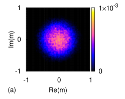
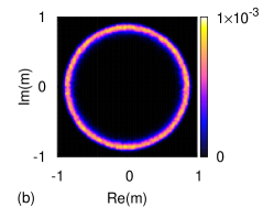
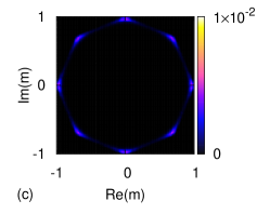
Figure 1: (Color online) Distributions of the order parameter $m$ on the complex plane, obtained for $p=1$, $q=8$, and $L=8$. We start from the high-temperature regime and then cool down the system slowly. Here are shown three characteristic distributions, where one finds (a) a disordered phase at temperature $T=1.50$, (b) a quasiliquid phase at $T=0.70$, and (c) an ordered phase at $T=0.36$, where the temperatures are given in units of $J/k_{B}$.

As in Ref. katz , it is instructive to visualize the distribution of $m$ on the complex plane. The distributions in Fig. 1 are obtained by running Monte Carlo simulations with the single-cluster update algorithm wolff ; janke ; hasen-sto , and each panel represents a different phase of the eight-state clock model at a different temperature. In the leftmost panel [Fig. 1(a)], we see the disordered phase in the high-temperature regime. The order parameter $m$ exhibits a two-dimensional Gaussian peak around the origin, which may be regarded as a delta peak at $|m|=0$ in the thermodynamic limit. Figure 1(b) illustrates the quasiliquid phase, where the order parameter rotates in the $\phi$ direction with nonzero magnitude. Note that both of the distributions in Figs. 1(a) and 1(b) manifest a continuous rotational symmetry, which is spontaneously broken at a lower temperature as shown in Fig. 1(c). One finds a true LRO being established so that $m$ indicates well-defined directions selected from the eight-fold symmetry.

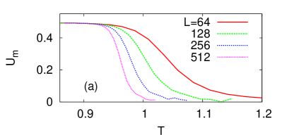
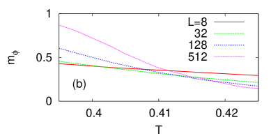
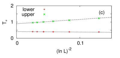
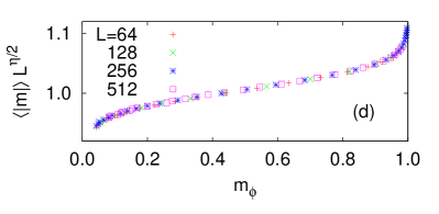
Figure 2: (Color online) Double phase transitions for $p=1$ and $q=8$. (a) The transition between quasiliquid and disordered phases is detected by merging of $U_{m}$ curves. (b) The other transition occurs between the ordered and quasiliquid phases, which is detected by $m_{\phi}$. (c) Extrapolating positions of inflection points according to the KT picture, we get $T_{c1}=0.417(3)$ and $T_{c2}=0.894(1)$. (d) Checking Eq. (7) with $\eta/2=0.031$, which best describes the data with a single curve.

A major difference between Figs. 1(a) and 1(b) lies in the distributions of $|m|$. The transition between the quasiliquid and disordered phases can be detected by means of Binder’s fourth-order cumulant,

$$U_{m}=1-\frac{\left<|m|^{4}\right>}{2\left<|m|^{2}\right>^{2}},$$ (3)

where $\left<\cdots\right>$ represents the thermal average [Fig. 2(a)]. The factor of two in the denominator of Eq. (3) is based on the fact that $\left<|m|^{4}\right>=2\left<|m|^{2}\right>^{2}$ for such a two-dimensional Gaussian distribution as in Fig. 1(a). We should note that $U_{m}$ does not detect the transition between the ordered and quasiliquid phases since they differ only in the angular direction on the complex plane. Henceforth, we need a quantity capturing the change along $\phi$. In the same spirit as $U_{m}$, one may define a cumulant as

$$U_{\phi}=1-\frac{5\left<\tilde{\phi}^{4}\right>}{9\left<\tilde{\phi}^{2}\right>^{2}},$$ (4)

where $\tilde{\phi}\equiv(2\pi)^{-1}(q\phi{\rm~{}mod~{}}2\pi)$ so that $U_{\phi}$ goes to zero when the distribution is uniform with respect to $\phi$. Or we may alternatively have

$$m_{\phi}=\left<\cos(q\phi)\right>,$$ (5)

which yields a finite value when $\phi$ is frozen but again vanishes when $\phi$ is isotropically distributed [Fig. 2(b)]. Provided that the system is nearly ordered with large enough $q$, we approximately have $\phi\approx N^{-1}\sum_{j}\theta_{j}$ from Eq. (2) so that $m_{\phi}\approx\left<\cos(2\pi\bar{n})\right>$ with $\bar{n}=N^{-1}\sum_{j}n_{j}$. By duality, the integer field $n_{j}$ can be mapped to a charge distribution in the lattice Coulomb gas savit and the approximate expression for $m_{\phi}$ has been introduced in Ref. hasen-sos2 to monitor the fugacity of charged particles under numerical renormalization-group calculations. Since the quasiliquid phase exists between the ordered and disordered phases for $q=8$, we have two separate transitions at $T=T_{c1}$ and $T_{c2}$, which are clearly detected by the above quantities. Note the movements of data points in Figs. 2(a) and 2(b) with different system sizes. Since the position of an inflection point, $T_{\ast}$, would correspond to where the transition occurs in the thermodynamic limit, we may extrapolate them according to the KT scenario,

$$\ln L\sim\left|T_{\ast}-T_{c}\right|^{-1/2},$$ (6)

to estimate the critical temperatures both for the upper and lower transitions [Fig. 2(c)]. In addition, regarding $\left<|m|\right>=L^{-\eta/2}\tilde{m}(L,T)$ around $T_{c1}$ challa , we replace the dependency on both of $L$ and $T$ by that on a single variable $m_{\phi}=m_{\phi}(L,T)$ so that

$$\left<|m|\right>=L^{-\eta/2}f(m_{\phi}).$$ (7)

In other words, plotting $\left<|m|\right>L^{\eta/2}$ against $m_{\phi}$, data from different sizes are expected to fall on a single curve if one correctly selects $\eta$. This provides a way to determine $\eta$ even without precise knowledge of $T_{c1}$ (see also Ref. loison ). The best fit is found at $\eta/2=0.031(2)$ as shown in Fig. 2(d), while the theoretical value is given as $\eta/2=1/32=0.03125$ at $T=T_{c1}$ elit .

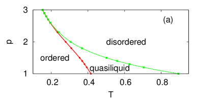
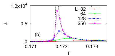
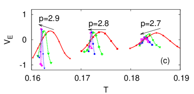
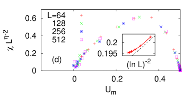
Figure 3: (Color online) (a) Phase diagram of the generalized eight-state clock model. (b) Susceptibility as a function of $T$ at $p=2.8$, where the dotted lines describe $\chi\sim|T-T_{c}|^{-1.2}$, with $T_{c}=0.17184$. (c) $V_{E}$ as a function of $T$. For each $p$, system sizes are given by $L=16,32,64$, and $128$ from right to left. (d) Estimation of $\eta$ for $p=2.6$ by Eq. (9). Seventh-order polynomials are used to find the best fit, from which $\eta=0.41(4)$ is estimated. Inset: $T_{c2}$ at $p=2.6$ against $(\ln L)^{-2}$ up to $L=512$. It moves slower than predicted by Eq. (6) as shown in comparison with the straight dotted line.

When altering the potential shape by increasing $p$ in Eq. (1), one may well expect that the two transitions will eventually transform into a single, discontinuous transition at a certain $p$ value as the Potts-model limit is approached. How this happens can be found by numerical simulations, and a phase diagram thereby obtained is shown in Fig. 3(a). It seems that the two phase-separation lines merge as $p$ approaches $3.0$. A better estimate is obtained by looking at magnetic susceptibility. Recalling that susceptibility $\chi=N(k_{B}T)^{-1}\left(\left<|m|^{2}\right>-\left<|m|\right>^{2}\right)$ corresponds to the sum of correlations, we may argue that its divergence implies long-ranged correlations over the system, a key feature of the quasiliquid phase. If $p$ is small enough to exhibit the quasiliquid phase, susceptibility indeed diverges over a finite temperature range. For $p=2.8$, however, we find that data points fall on $\chi\sim|T-T_{c}|^{-1.2}$ which has only one singular point at $T=T_{c}$ [Fig. 3(b)]. This $T_{c}$ is also consistent with the results from $U_{m}$ and $m_{\phi}$. We therefore conclude that the quasiliquid phase shrinks to a single point at $p\simeq 2.8$. Furthermore, the distribution of energy per spin, $E$, exhibits double peaks for $p\gtrsim 2.8$. By analogy with $U_{m}$, we introduce the following quantity:

$$V_{E}=1-\frac{\left<\left(E-\left<E\right>\right)^{4}\right>}{3\left<\left(E-\left<E\right>\right)^{2}\right>^{2}}.$$ (8)

Recall that if a scalar variable $x$ has a one-dimensional Gaussian distribution with zero mean, one readily finds $\left<x^{4}\right>=3\left<x^{2}\right>^{2}$. Consequently, $V_{E}$ will vanish when there exists a single peak positioned at $\left<E\right>$. It will approach a nontrivial value, however, when the energy distribution has double peaks on opposite sides of the average value $\left<E\right>$. A similar attempt to define such a quantity has already been made in Ref. challa for characterizing a discontinuous transition. Figure 3(c) shows that $V_{E}$ remains finite at $p\gtrsim 2.8$, which signals a change to a discontinuous transition cardy ; domany1 .

The concept of universality suggests that the critical properties will be kept the same in the vicinity of $p=1$. However, one may ask if the natures of the transitions between the ordered and quasiliquid phases and between the quasiliquid and disordered phases depend on the value of $p$. Applying Eq. (7) to higher $p$ values, we find that $\eta=1/16$ cannot be ruled out even when $p$ approaches $2$. However, the quality of fit severely deteriorates at $p$ higher than $2$, possibly due to that our magnetization data are easily influenced by the proximity of the upper transition. On the other hand, with the same motivation as in Eq. (7), we may characterize the upper transition by means of the following scaling relation loison :

$$\chi=L^{2-\eta}g(U_{m}).$$ (9)

This method yields $\eta=0.24(1)$ at $p=1.0$ in agreement with the prediction of $1/4=0.25$ for the KT transition kos . It is not very surprising that $\eta$ tends to be underestimated here if taking into account the logarithmic correction involved in susceptibility kenna ; hasen . We observe from our numerical data that the criticality deviates from the standard KT type below the merging point. If we take $p=2.6$, for instance, the best fit is found at $\eta=0.41$ and the size dependence of the transition temperatures deviates from Eq. (6) [Fig. 3(d)]. Still, it remains to be investigated in detail how the critical behavior begins to change or if the standard KT behavior is recovered for even larger lattice sizes ($L>512$) in spite of the data collapse shown in Fig. 3(d) for lattice sizes up to $L=512$.

In summary, we have proposed a practical quantity to distinguish the true and quasi LROs, based on the order-parameter distribution. Using this quantity, we have provided a phase diagram on the $p-T$ plane for the generalized eight-state clock model. It has been shown that a discontinuous transition appears when the phase-separation lines merge into one at $p\simeq 2.8$. We have also checked critical properties along the lines and found changes in scaling behaviors before reaching the merging point from numerical calculations up to $L=512$.

- (1) J. M. Kosterlitz, J. Phys. C 7, 1046 (1974).
- (2) J. M. Kosterlitz and D. J. Thouless, J. Phys. C 6, 1181 (1973).
- (3) P. Minnhagen, Rev. Mod. Phys. 59, 1001 (1987).
- (4) H. J. F. Knops, Phys. Rev. Lett. 39, 766 (1977).
- (5) M. Hasenbusch, J. Stat. Mech.: Theory Exp. 2008, P08003.
- (6) M. Hasenbusch, M. Marcu, and K. Pinn, Physica A 208, 124 (1994).
- (7) M. Hasenbusch and K. Pinn, J. Phys. A 30, 63 (1997).
- (8) C. M. Lapilli, P. Pfeifer, and C. Wexler, Phys. Rev. Lett. 96, 140603 (2006).
- (9) E. Domany, M. Schick, and R. H. Swendsen, Phys. Rev. Lett. 52, 1535 (1984).
- (10) F. Y. Wu, Rev. Mod. Phys. 54, 235 (1982).
- (11) J. L. Cardy, J. Phys. A 13, 1507 (1980).
- (12) E. Domany, D. Mukamel, and A. Schwimmner, J. Phys. A 13, L311 (1980).
- (13) J. V. José, L. P. Kadanoff, S. Kirkpatrick, and D. R. Nelson, Phys. Rev. B 16, 1217 (1977).
- (14) S. Elitzur, R. B. Pearson, and J. Shigemitsu, Phys. Rev. D 19, 3698 (1979).
- (15) R. Savit, Rev. Mod. Phys. 52, 453 (1980).
- (16) K. Binder and D. W. Heermann, Monte Carlo Simulation in Statistical Physics, 2nd ed. (Springer-Verlag, Berlin, 1992).
- (17) D. R. Nelson and J. M. Kosterlitz, Phys. Rev. Lett. 39, 1201 (1977).
- (18) P. Minnhagen and G. G. Warren, Phys. Rev. B 24, 2526 (1981).
- (19) P. Minnhagen and B. J. Kim, Phys. Rev. B 67, 172509 (2003).
- (20) M. S. S. Challa and D. P. Landau, Phys. Rev. B 33, 437 (1986).
- (21) Y. Tomita and Y. Okabe, Phys. Rev. B 65, 184405 (2002).
- (22) H. G. Katzgraber and A. P. Young, Phys. Rev. B 64, 104426 (2001).
- (23) U. Wolff, Phys. Rev. Lett. 62, 361 (1989).
- (24) W. Janke and K. Nather, Phys. Rev. B 48, 7419 (1993).
- (25) H. G. Evertz, M. Hasenbusch, M. Marcu, K. Pinn, and S. Solomon, Phys. Lett. B 254, 185 (1991).
- (26) M. S. S. Challa, D. P. Landau, and K. Binder, Phys. Rev. B 34, 1841 (1986).
- (27) D. Loison, J. Phys.: Condens. Matter 11, L401 (1999).
- (28) R. Kenna and A. C. Irving, Phys. Lett. B 351, 273 (1995).
- (29) M. Hasenbusch, J. Phys. A 38, 5869 (2005).