Pulse Shaping, Localization and the Approximate Eigenstructure of LTV Channels

Abstract

In this article we show the relation between the theory of pulse shaping for WSSUS channels and the notion of approximate eigenstructure for time–varying channels. We consider pulse shaping for a general signaling scheme, called Weyl–Heisenberg signaling, which includes OFDM with cyclic prefix and OFDM/OQAM. The pulse design problem in the view of optimal WSSUS–averaged SINR is an interplay between localization and ”orthogonality”. The localization problem itself can be expressed in terms of eigenvalues of localization operators and is intimately connected to the concept of approximate eigenstructure of LTV channel operators. In fact, on the $\mathcal{L}_{2}$–level both are equivalent as we will show. The concept of ”orthogonality” in turn can be related to notion of tight frames. The right balance between these two sides is still an open problem. However, several statements on achievable values of certain localization measures and fundamental limits on SINR can already be made as will be shown in the paper.

I Introduction

Optimal signaling through linear time–varying (LTV) channels is a challenging task for future communication systems. For a particular realization of the time–varying channel operator the transmitter and receiver design which avoids crosstalk between different time–frequency slots is related to ”eigen–signaling” which simplifies much the information theoretic treatment of communication in dispersive channels. But it is well–known that for an ensemble of channels which are dispersive in time and frequency (doubly–dispersive) such a joint separation of the subchannels can not be achieved because the eigen decompositions can differ from one to another channel realization. Several approaches are proposed to describe ”eigen”–signaling in some approximate sense. However, then a necessary prerequisite is the characterization of approximation errors.

A typical scenario, present for example in wireless communication, is signaling through a random doubly–dispersive channel, represented by the operator $\boldsymbol{{\mathcal{H}}}$. The received signal $r:\mathbb{R}\rightarrow\mathbb{C}$ at time instant $t$ is then:

$$r(t)=(\boldsymbol{{\mathcal{H}}}s)(t)+n(t)$$

A preferred design of the transmit signal $s:\mathbb{R}\rightarrow\mathbb{C}$ needs knowledge on the true eigenstructure of the channel operator $\boldsymbol{{\mathcal{H}}}$. This would in principle allow interference–free transmission and simple recovering algorithms of the information from received signal $r$ degraded by the noise process $n$. However, for $\boldsymbol{{\mathcal{H}}}$ being a random operator, a random eigenstructure has to be expected in general such that a joint design of the transmitter and the receiver for an ensemble of channels has to be performed. Nevertheless, interference can then not be avoided and remains in the communication chain. For such interference scenarios bounds on the distortion of a particular selected signaling scheme are mandatory for reliable system design.

This problem has been considered, for example, already in [1] and [2]. The investigation of the $\mathcal{L}_{p}$–norm $E_{p}$ of the error $\boldsymbol{{\mathcal{H}}}s-\lambda r$ for $\lambda\in\mathbb{C}$ enables us to improve and generalize recent results in this direction. We will focus in this article on the results for $p=2$ which show the important relation to pulse shape optimization for Weyl–Heisenberg signaling [3, 4, 5]. We will use this generalized description of a multicarrier system and consider in this framework the channel averaged ”signal to interference and noise ratio”. To perform this average we will use the wide–sense stationary uncorrelated scattering (WSSUS) channel model.

The paper is organized as follows. In Section II we will review the basics from time–frequency analysis, introduce the spreading representation of doubly–dispersive channels and consider the problem of controlling the approximation error $E_{2}$. In Section III we will focus on the description of multicarrier transmission and WSSUS pulse shape optimization. We demonstrate the relation to $E_{2}$. In Section IV we give several relations to the ”size” (Lebesgue measure) $|U|$ of the support $U$ in the time–frequency plane of the channel’s spreading function. In the last part we will verify our framework with some numerical tests.

II Time–Varying Channels

II-A Time–Frequency Shifts

The fundamental operations on a signal $\gamma:\mathbb{R}\rightarrow\mathbb{C}$ caused by the time–varying nature of typical wireless channels are time–frequency shifts. Let us denote a displacement in time by $\mu_{1}$ and in frequency by $\mu_{2}$ by the operator ${\boldsymbol{S}}_{\mu}$ defined as:

$$({\boldsymbol{S}}_{\mu}\gamma)(t):=e^{i2\pi\mu_{2}t}\gamma(t-\mu_{1})$$ (1)

($i$ is the imaginary unit and $\mu=(\mu_{1},\mu_{2})$). These operators act isometrically on the $\mathcal{L}_{p}(\mathbb{R})$ spaces, hence unitary on the Hilbert space $\mathcal{L}_{2}(\mathbb{R})$. The abstract action of ${\boldsymbol{S}}_{\mu}$ onto a function $\gamma$ is observable for example as a correlation response with another function $g$. In this way the (cross) ambiguity function:

$${\mathbf{A}}_{g\gamma}(\mu)\overset{\text{def}}{=}\langle g,{\boldsymbol{S}}_{\mu}\gamma\rangle=\int_{\mathbb{R}}\bar{g}(x)\gamma(x-\mu_{1})e^{i2\pi\mu_{2}x}dx$$ (2)

can be defined as an observable quantity. Definition (1) is not unique and corresponds to a particular polarization in the Weyl–Heisenberg group (see [6, 7]).

A fundamental operation in time–frequency analysis is the symplectic Fourier transform $\mathcal{F}_{s}$ defined for a function $f:\mathbb{R}^{2}\rightarrow\mathbb{C}$ as

$$(\mathcal{F}_{s}f)(\mu)=\int_{\mathbb{R}^{2}}e^{-i2\pi\eta(\nu,\mu)}f(\nu)d\nu$$ (3)

where $\eta(\nu,\mu):=\nu_{1}\mu_{2}-\nu_{2}\mu_{1}$ is called the symplectic form. (3) differs from ordinary Fourier transform only by coordinate/sign switching which quite intuitive because time–shifts $\mu_{1}$ cause oscillations in frequency where frequency shifts $\mu_{2}$ cause them in time. Then the (cross) Wigner distribution is the symplectic Fourier transform of the (cross) ambiguity function.

II-B Spreading Representation of Doubly–Dispersive Channels

Doubly–dispersive channels are physically characterized by scattering in the time–varying environment. Typically one defines therefore the channel operator $\boldsymbol{{\mathcal{H}}}$ weakly in terms of the transmit and receive filters $\gamma$ and $g$ of a particular communication device as:

$$\langle g,\boldsymbol{{\mathcal{H}}}\gamma\rangle=\int_{\mathbb{R}^{2}}\boldsymbol{\Sigma}_{\boldsymbol{{\mathcal{H}}}}(\mu){\mathbf{A}}_{g\gamma}(\mu)d\mu$$ (4)

The function $\boldsymbol{\Sigma}_{\boldsymbol{{\mathcal{H}}}}:\mathbb{R}^{2}\rightarrow\mathbb{C}$ is then called the spreading function of the channel operator $\boldsymbol{{\mathcal{H}}}$. Its symplectic Fourier transform, $\boldsymbol{L}_{\boldsymbol{{\mathcal{H}}}}=\mathcal{F}_{s}\boldsymbol{\Sigma}_{\boldsymbol{{\mathcal{H}}}}$, is called the symbol of $\boldsymbol{{\mathcal{H}}}$. The practical assumption that the support $U\subset\mathbb{R}^{2}$ of $\boldsymbol{\Sigma}_{\boldsymbol{{\mathcal{H}}}}$ is compact renders $\boldsymbol{{\mathcal{H}}}$ to be a Hilbert–Schmidt operator whenever $\boldsymbol{\Sigma}_{\boldsymbol{{\mathcal{H}}}}$ is bounded and $|U|>0$ (single– or non–dispersive channels have $|U|=0$). In this paper we will restrict the analysis to those channels to avoid the use of distributions. To this end, let us call $\text{OP}(U)$ as the set of channel operators $\boldsymbol{{\mathcal{H}}}$ having a spreading function $\boldsymbol{\Sigma}_{\boldsymbol{{\mathcal{H}}}}$ with non–zero and finite support in $U$ where $0<|U|<\infty$.

II-C Approximate Eigenstructure

It is a fundamental question, how well we can describe the action of the channel in terms of its symbol. More generally speaking, how valid is an approximation of the form:

$$\boldsymbol{{\mathcal{H}}}{\boldsymbol{S}}_{\mu}\gamma\approx\lambda(\mu){\boldsymbol{S}}_{\mu}g$$ (5)

See for example [8] for recent applications of this approximation. For example, for $g$ and $\gamma$ being singular functions of $\boldsymbol{{\mathcal{H}}}$ (eigenfunctions of $\boldsymbol{{\mathcal{H}}}\boldsymbol{{\mathcal{H}}}^{*}$ and $\boldsymbol{{\mathcal{H}}}^{*}\boldsymbol{{\mathcal{H}}}$) there is equality for a particular $\lambda(0)$ (the singular value). However, this is not well suited for our formulation, because $\boldsymbol{{\mathcal{H}}}$ will be a random channel operator as for example further described in Section II-D. However, if we restrict the set of operators to be from class $\text{OP}(U)$ we can seek for $g$ and $\gamma$ which are independent of the channel realization and reasonable bound the approximation error $E_{p}=\lVert\boldsymbol{{\mathcal{H}}}{\boldsymbol{S}}_{\mu}\gamma-\lambda(\mu){\boldsymbol{S}}_{\mu}g\rVert_{p}$. For a single $\boldsymbol{{\mathcal{H}}}$ we will call this setup as approximate eigenstructure and in this article we will consider $p=2$ because of its relation to pulse design (considered in Section III). For more general results see [7]. Our problem is:

Problem 1

Let be $\boldsymbol{{\mathcal{H}}}\in\text{OP}(U)$ and $\lVert g\rVert_{2}=\lVert\gamma\rVert_{2}=1$ and $1\leq a\leq\infty$. Let $\delta\in\mathbb{R}_{+}$ be independent of $\boldsymbol{\Sigma}_{\boldsymbol{{\mathcal{H}}}}^{(\alpha)}$ such that

$$\begin{split}E_{2}\leq\delta\cdot\lVert\boldsymbol{\Sigma}_{\boldsymbol{{\mathcal{H}}}}\rVert_{a}\end{split}$$ (6)

How small can we choose $\delta$ given $g$, $\gamma$, $U$ and $a$ ? What can be said about $\inf_{g,\gamma}(\delta)$ given $U$ and $a$.

Note that this formulation comprises a joint approximate eigenstructure for all channels $\boldsymbol{{\mathcal{H}}}\in\text{OP}(U)$ but with individual bounds $\delta\cdot\lVert\boldsymbol{\Sigma}_{\boldsymbol{{\mathcal{H}}}}^{(\alpha)}\rVert_{a}$ for the approximation error.

First decompositions results in this field can be found already in the literature on pseudodifferential operators [9, 6]. More recent results with direct application to time–varying channels were obtained by Kozek [3] and Matz [10] which resemble the notion of underspread channels. They found results on $\delta$ for $\lambda=\boldsymbol{L}_{\boldsymbol{{\mathcal{H}}}}$ and $a=1$ which follow from the approximate product rule in terms of Weyl symbols. This estimate intimately scales with $|U|$ and breaks down at a certain critical size. Channels below this critical size are called in their terminology underspread, otherwise overspread. However, the critical term in their estimate can be dropped and the overall result can be improved to $\delta^{2}\leq 2\lVert(1-{\mathbf{A}}_{g\gamma})\chi_{U}\rVert_{\infty}$ [7]. Similar estimates can be obtained for other weight functions instead of $\chi_{U}$ (the characteristic function of $U$). For this case ($a=1$) it is difficult to separate explicit relations on $|U|$. However, as will be shown, for $a>1$ this can be done.

With the choice $\lambda=\boldsymbol{L}_{\boldsymbol{{\mathcal{H}}}}$ a formulation independent of $g$ and $\gamma$ is achieved. An approach which is better suited for our application instead is

$$\lambda(\mu)=\langle{\boldsymbol{S}}_{\mu}g,\boldsymbol{{\mathcal{H}}},{\boldsymbol{S}}_{\mu}\gamma\rangle=\mathcal{F}_{s}(\boldsymbol{\Sigma}_{\boldsymbol{{\mathcal{H}}}}{\mathbf{A}}_{g\gamma})(\mu)$$ (7)

This choice is also known as the orthogonal distortion (smoothing with the cross Wigner function) and corresponds to the $E_{2}$ minimizer in (6) for fixed $g$ and $\gamma$. This approach was also already considered for $g=\gamma$ in [2]. One can prove the following Lemma [7]:

Lemma 1

Let $1<a\leq\infty$ and $1/a+1/b=1$ and $\boldsymbol{\Sigma}_{\boldsymbol{{\mathcal{H}}}}\in\mathcal{L}_{a}(\mathbb{R}^{2})$. If $|U|\leq 1$ it holds

$$\frac{E_{2}}{\lVert\boldsymbol{\Sigma}_{\boldsymbol{{\mathcal{H}}}}\rVert_{a}}\leq\left(|U|-\int_{U}|{\mathbf{A}}_{g\gamma}(\mu)|^{2}d\mu\right)^{1/\max(b,2)}$$ (8)

Similar bounds can be found for all $p$–norms with $2\leq p<\infty$ and more detailed results avoid also the constraint $|U|\leq 1$.

II-D WSSUS Scattering

A common statistical model for random doubly–dispersive channels is the WSSUS channel model, originally introduced by Bello [11]. In this model the spreading function $\boldsymbol{\Sigma}_{\boldsymbol{{\mathcal{H}}}}$ is described as a zero–mean 2D–random process uncorrelated at different arguments, which gives:

$${\mathbf{E}}\{|\langle g,\boldsymbol{{\mathcal{H}}}\gamma\rangle|^{2}\}=\int_{\mathbb{R}^{2}}\boldsymbol{C}(\mu)|{\mathbf{A}}_{g\gamma}(\mu)|^{2}d\mu$$ (9)

The (non–negative) function $\boldsymbol{C}:\mathbb{R}^{2}\rightarrow\mathbb{R}_{+}$ is called the scattering function. Let be $\lVert\boldsymbol{C}\rVert_{1}=1$. Then $\boldsymbol{C}(\mu)$ is also the probability density for the occurrence of a time–frequency shift $\mu$ in the channel. In time–frequency analysis the term $\langle\boldsymbol{C},|{\mathbf{A}}_{g\gamma}|^{2}\rangle$ in (9) is sometimes also called the modulation 2–norm [12] of $\gamma$ with respect to window $g$ and weight function $\sqrt{\boldsymbol{C}}$.

III Signaling and Pulse Shaping

In Lemma 8 and (9) we have already shown certain localization measures characterizing the signal distortion in time–varying channels, in particular for the WSSUS model. In this section we will now establish a simple communication chain, including OFDM and OQAM/OFDM, which use $g$ and $\gamma$ as corresponding transmit and receiver filters. Finally, we aim at a relation between $\{g,\gamma\}$, the WSSUS–averaged SINR and the role of time–frequency localization which is relevant for $E_{2}$.

III-A Weyl–Heisenberg Signaling

Conventional OFDM and pulse shaped OQAM/OFDM can be formulated jointly within the concept of Weyl–Heisenberg signaling [13]. To avoid cumbersome notation we will adopt a two–dimensional index notation $n=(n_{1},n_{2})\in{\mathbb{Z}}^{2}$ for time–frequency slots $n$, such that the baseband transmit signal is

$$s(t)=\sum_{n\in{\mathcal{I}}}x_{n}\gamma_{n}(t)=\sum_{n\in{\mathcal{I}}}x_{n}({\boldsymbol{S}}_{\Lambda n}\,\gamma)(t)$$ (10)

where $\Lambda{\mathbb{Z}}^{2}$ is a lattice ($\Lambda$ denotes its $2\times 2$ real generator matrix) with $|\Lambda|:=|\det(\Lambda)|>0$. The indices $n$ range over the doubly-countable set ${\mathcal{I}}\subset{\mathbb{Z}}^{2}$, referring to the data burst to be transmitted. In practice $\Lambda$ is often restricted to be diagonal, i.e. $\Lambda=\text{diag}(T,F)$. Other lattices are considered for example in [14]. The efficiency (in complex symbols) of the signaling is $|\Lambda|^{-1}$. The coefficients $x_{n}$ are the complex data symbols at time instant $n_{1}$ and subcarrier index $n_{2}$ (from now on $\,\bar{\cdot}$ always denotes complex conjugate and $\cdot^{*}$ means conjugate transpose), where $\boldsymbol{x}=(\dots,x_{n},\dots)^{T}$. By introducing the elements $H_{m,n}:=\langle g_{m},\boldsymbol{{\mathcal{H}}}\gamma_{n}\rangle$ of the channel matrix $H$ the multicarrier transmission can be formulated as the linear equation $\tilde{\boldsymbol{x}}=H\boldsymbol{x}+\tilde{\boldsymbol{n}}$, where $\tilde{\boldsymbol{n}}=(\dots,\langle g_{m},n\rangle,\dots)^{T}$ is the vector of the projected noise having variance ${\sigma^{2}}:={\mathbf{E}}\{|\langle g_{m},n\rangle|^{2}\}$ per component.

III-B Complex Signaling and OFDM

The classical OFDM system exploiting a cyclic prefix (cp-OFDM) is obtained by assuming a lattice generated by $\Lambda=\text{diag}(T,F)$ and $\gamma(t)\sim\chi_{[-T_{cp},T_{u}]}(t)$ which is (up to normalization) the characteristic function of the interval $[-T_{cp},T_{u}]$. $T_{u}$ usually denotes the duration of the useful part of the signal and $T_{cp}$ is the length of the cyclic prefix such that $T=T_{u}+T_{cp}$. The OFDM subcarrier spacing is $F=1/T_{u}$. At the receiver the rectangular pulse $g(t)\sim\chi_{[0,T_{u}]}(t)$ is used which removes the cyclic prefix. The efficiency is given as $|\Lambda|^{-1}=T_{u}/(T_{u}+T_{cp})<1$. It can be easily verified that ${\mathbf{A}}_{g\gamma}(\mu+\Lambda m)\sim\delta_{m,0}$ if $0\leq\mu_{1}\leq T_{cp}$ and $\mu_{2}=0$ (or see [15] for the full formula). Thus, orthogonality is preserved in time–invariant channels with maximum delay smaller than $T_{cp}$, but at the cost of signal power (the redundancy is not used) and efficiency.

III-C Real Signaling and OQAM

For those schemes an inner product ${\text{Re}}\{\langle\cdot,\cdot\rangle\}$ and $\Lambda=\text{diag}(T,F)$ having $|\Lambda|=1/2$ is considered, which is realized by OQAM based modulation for OFDM (OQAM/OFDM) [16]. Before modulation the mapping $x_{n}=i^{n}x^{\text{R}}_{n}$ has to be applied, where $x^{\text{R}}_{n}\in\mathbb{R}$ is the real-valued information to transmit. After demodulation $\tilde{x}^{\text{R}}_{m}={\text{Re}}\{i^{-m}\tilde{x}_{m}\}$ is performed. Moreover, the pulses $(g,\gamma)$ have to be real. Thus, formally the transmission of the real information vector $\boldsymbol{x}^{\text{R}}=(\dots,x^{\text{R}}_{n},\dots)^{T}$ can be written as $\tilde{\boldsymbol{x}}^{\text{R}}=H^{\text{R}}\boldsymbol{x}^{\text{R}}+\tilde{\boldsymbol{n}}^{\text{R}}$ where the real channel matrix elements are:

$$H^{\text{R}}_{m,n}={\text{Re}}\{i^{n-m}H_{m,n}\}={\text{Re}}\{i^{n-m}\langle g_{m},\boldsymbol{{\mathcal{H}}}\gamma_{n}\rangle\}$$ (11)

and ”real–part” noise components are $\tilde{n}^{\text{R}}_{m}={\text{Re}}\{i^{-m}\langle g_{m},n\rangle\}$. There exists no such orthogonality property for OQAM based signaling as for cp-OFDM in time–invariant channels, but biorthogonality of the form $\Re\{\langle g_{m},\gamma_{n}\rangle\}\sim\delta_{m,n}$ can be achieved. It is known that the design of (bi–)orthogonal OQAM signaling is implicitly related to (bi–) orthogonal Wilson bases [17] which is in turn equivalent to the computation of (dual–) tight frames [18].

While the system operates with real information at $\epsilon=2$ the effective efficiency is one, which has advantages in the view of pulse shaping as will explained later on.

III-D A Lower Bound on the WSSUS Averaged SINR

In multicarrier transmission most commonly one–tap equalization per time–frequency slot is considered, hence it is naturally to require ${\mathbf{E}}\{|H_{m,m}|^{2}\}$ to be maximal and the averaged interference power from all other lattice points to be minimal as possible. For real schemes $H_{m,m}$ has to be replaced by $H^{\text{R}}_{m,n}$ from (11). For $\lVert\boldsymbol{C}\rVert_{1}=1$, $\lVert g\rVert_{2}=\lVert\gamma\rVert_{2}=1$ and ${\mathbf{E}}\{\bar{x}_{m}x_{n}\}=\delta_{m,n}$ we have shown in [4] that the averaged ”signal to interference and noise ratio” is lower bounded by:

$$\text{\small{\rm{SINR}}}(g,\gamma,\Lambda)\geq\frac{\langle\boldsymbol{C},|{\mathbf{A}}_{g\gamma}|^{2}\rangle}{{\sigma^{2}}+B_{\gamma}-\langle\boldsymbol{C},|{\mathbf{A}}_{g\gamma}|^{2}\rangle}$$ (12)

with equality for $\{\gamma_{m}\}$ forming a tight frame (more details and references on frame theory in [4]). The constant $B_{\gamma}=\rho(S_{\gamma,\Lambda})$ is the spectral radius of the positive semidefinite operator $S_{\gamma,\Lambda}$ defined as:

$$(S_{\gamma,\Lambda}f)(t):=\sum_{\lambda\in\Lambda{\mathbb{Z}}^{2}}\langle{\boldsymbol{S}}_{\lambda}\gamma,f\rangle({\boldsymbol{S}}_{\lambda}\gamma)(t)$$

The minimal $B_{\gamma}$ is $\max(|\Lambda|^{-1},1)$ which is achieved for tight frames in the case of $|\Lambda|\leq 1$ and for incomplete orthogonal bases in the case of $|\Lambda|>1$. In addition to complex signaling as considered in Section III-B Equation (12) holds for real signaling (Section III-C) as well if the spreading function and the noise are circular–symmetric processes [4].

III-E SINR Optimization and the Pulse Shaping Problem

It follows that maximizing the bound in (12) is an interplay between two criteria: localization (maximizing $\langle\boldsymbol{C},|{\mathbf{A}}_{g\gamma}|^{2}\rangle$) and ”orthogonality”, respectively ”tightness” (minimizing $B_{\gamma}$). Orthogonalization is only possible for $|\Lambda|\geq 1$. For $|\Lambda|\leq 1$ a tight frame has to be constructed. However, with the notion of the adjoint lattice $\Lambda^{\circ}:=|\Lambda|^{-1}\Lambda$ both cases are dual in the sense of Ron and Shen [19], which means that we can limit ourself to the case $|\Lambda|\leq 1$.

One possible method [14, 4] to achieve a minimal $B_{\gamma}$ in a $\mathcal{L}_{2}$–optimal sense is to apply $O:=\left(|\Lambda|\cdot S_{\gamma,\Lambda}\right)^{-\frac{1}{2}}$ on the result of a localization procedure to obtain $\gamma^{\circ}=O\gamma$ (for $|\Lambda|>1$ a similar procedure follows from replacing $\Lambda$ by $\Lambda^{\circ}$). For example, in [20] it was shown that IOTA (Isotropic Orthogonal Transform Algorithm, $\Lambda=\text{diag}(T,F)$ with $|\Lambda|=1/2$) as proposed in [21] is equivalent to $O$ applied on a Gaussian. In combination with OQAM modulation as introduced in section III-C this is also an orthogonal signaling (in the absence of a channel). The advantage of this approach is that at $|\Lambda|=1/2$ the operation $O$ is quite stable. In contrast: optimal efficiency with orthogonal (or bi–orthogonal) complex signaling (this implies $|\Lambda|=1$) is always affected by the Balian–Low Theorem (BLT) (see for example [22]), i.e. $O$ is unbounded if it exists.

Estimates on the localization penalty of the operation $O$ on the SINR are in general related to mapping properties of $O$ on modulation spaces [12]. Beside the general problem of invertibility of the operator in (III-D) (for recent results see here for example [23] or [22]) there remains the open question on optimal constants which are necessary to draw conclusions on the SINR.

IV Localization and Support Bounds

IV-A Pulse Shaping and Approximate Eigenstructure

The detailed knowledge of the scattering function of an statistical ensemble of channels can improve the overall performance of a communication device [4]. However, also this statistical parameters change over time in realistic applications. A more reliable assumption is the support knowledge only, i.e. a scattering function which is the normalized indicator function $\boldsymbol{C}=\chi_{U}/|U|$ of $U$. We then see that approximate eigenstructure in the formulation given in Lemma 8 and the localization aspect (the term $\langle\boldsymbol{C},|{\mathbf{A}}_{g\gamma}|^{2}\rangle$) of pulse shaping (12) are the same problems.

IV-B Localization Operators

Since $|{\mathbf{A}}_{g\gamma}|^{2}$ is quadratic in $\gamma$ we can rewrite $\langle|{\mathbf{A}}_{g\gamma}|^{2},\boldsymbol{C}\rangle=\langle\gamma,L_{\boldsymbol{C},g}\gamma\rangle$ where this quadratic form defines (weakly) an operator $L_{\boldsymbol{C},g}$. Such operators are also called localization operators [24]. $L_{\boldsymbol{C},g}$ is compact which follows from our assumptions on $\boldsymbol{C}$, such that

$$\max_{\gamma}\langle|{\mathbf{A}}_{g\gamma}|^{2},\boldsymbol{C}\rangle=\lambda_{\max}(L_{\boldsymbol{C},g})$$ (13)

This means that for fixed $g$ the optimal transmit pulse $\gamma$ is given by an eigenfunction corresponding to the maximal eigenvalue of $L_{\boldsymbol{C},g}$. The latter can also be reversed, i.e. for fixed $\gamma$ the optimal receive filter $g$ is determined.

$$\max_{g}\langle|{\mathbf{A}}_{g\gamma}|^{2},\boldsymbol{C}\rangle=\lambda_{\max}(L_{\tilde{\boldsymbol{C}},\gamma})$$ (14)

where $\tilde{\boldsymbol{C}}(\mu)=\boldsymbol{C}(-\mu)$. The eigenvalues and eigenfunctions of Gaussian ($g$ is set to be a Gaussian) localization operators on the disc ($U$ is a disc) or more generally with $\boldsymbol{C}$ having elliptical symmetry are known to be Hermite functions [24]. Kozek [3] found that for elliptical symmetry also the joint optimization ($g$ and $\gamma$) results in Hermite functions. Explicitely known is the joint optimum for $\boldsymbol{C}$ being Gaussian [5]. In (13) there is an invariance with respect to (affine) canonical transformations. See for example [6] for a review on the metaplectic representation. Essentially, this means that we can translate, rotate and shear $\boldsymbol{C}$ into some prototype shape being canonical equivalent but with further symmetries.

Focusing now on localization operators $L_{\boldsymbol{C},\gamma}$ with $\boldsymbol{C}:=\chi_{U}/|U|$ and let be $\lambda_{\max}:=\lambda_{\max}(L_{\boldsymbol{C},\gamma})$. One can show the following result:

Lemma 2

Let $U$ canonical equivalent to square. Then:

$$\frac{\text{erf}(\sqrt{\pi|U|/4})^{4}}{|U|^{2}}\leq\sup_{\lVert\gamma\rVert_{2}=1}\lambda_{\max}<\min(e^{-\frac{|U|}{e}},|U|^{-1})$$ (15)

The upper bound is general and holds for any shape.

The proof can be found in [7]. The upper bound can also be found in [5]. The lower bound can be calculated for other shapes (like a disc) as well. As a result for Problem 1 it follows from Lemma 8 that:

$$E_{2}\leq\lVert\boldsymbol{\Sigma}_{\boldsymbol{{\mathcal{H}}}}\rVert_{a}\cdot\left(|U|-\text{erf}(\sqrt{\pi|U|/4})^{2}\right)^{1/\max(b,2)}$$ (16)

IV-C Bounds for SINR

On the other hand, from the previous results we are also able to obtain for $|\Lambda|\leq 1$ an upper bound on SINR as follows. Assume that $\{\gamma_{n}\}_{n\in{\mathbb{Z}}^{2}}$ establishes a frame. Then we can compute $\gamma^{\circ}=O\gamma$ to obtain a tight frame $\{\gamma^{\circ}_{n}\}_{n\in{\mathbb{Z}}^{2}}$ with $B_{\gamma^{\circ}}=|\Lambda|^{-1}$. For a tight frame holds equality in (12). It remains to find the optimal $g$ which can be found for example as the maximizing (generalized) eigenvalue as shown in [4] (see also Section V-A). Let us call $\text{\small{\rm{SINR}}}^{*}:=\max_{g}\text{\small{\rm{SINR}}}(g,\gamma^{\circ},\Lambda)$. The upper bound in (15) of Lemma 2 gives then for $|U|\leq e$ that:

$$\text{\small{\rm{SINR}}}^{*}\leq\left(({\sigma^{2}}+|\Lambda|^{-1})e^{\frac{|U|}{e}}-1\right)^{-1}$$ (17)

Effectively, the upper bound (17) represents the assumption that we would be able to retain with $\gamma\rightarrow\gamma^{\circ}$ the localization upper bounded by the rhs of (15), thus ignoring the loss due to the BLT. This approach is valid to obtain an upper bound.

As already discussed at the end of Section III-E, in general no quantitative estimates exists on the localization loss, i.e. it is unknown to what degree (17) is achievable. Assuming negligible localization loss (”no BLT”) the lhs of (15) gives us also that:

$$\text{\small{\rm{SINR}}}^{*}\overset{\text{no BLT}}{\geq}\left(({\sigma^{2}}+|\Lambda|^{-1})\frac{|U|}{\text{erf}(\sqrt{\pi|U|/4})^{4}}-1\right)^{-1}$$ (18)

For uncritical $\Lambda$ (or $\Lambda^{\circ}$ respectively) the mapping $O$ can be well conditioned (which still depends on $\gamma$) such that (18) is an estimate of achievable values of $\text{\small{\rm{SINR}}}^{*}$. Our numerical results, shown in Section V-C, support these assumptions for $|\Lambda|=1/2$.

V Localization Algorithms and Numerical Verification

A well–known approach is to adapt the lattice $\Lambda$ and the time-/frequency spreads $\sigma_{t}$ and $\sigma_{f}$ of the pulses to the scattering function $\boldsymbol{C}$ of an ensemble of WSSUS channels where the device should operate. In practice various environments have to be classified by their spread in delay ($\boldsymbol{C}_{t}$) and mobility (spread $\boldsymbol{C}_{f}$ in two–sided Doppler frequencies) such that a potential mobile device will support a group of different modes $\{g,\gamma,\Lambda\}$. For $\Lambda=\text{diag}(T,F)$ this means to fulfill essentially $T/F\approx\sigma_{t}/\sigma_{f}\approx\boldsymbol{C}_{t}/\boldsymbol{C}_{f}$ which is known as ”pulse and grid scaling” [3, 25, 4]. However, up to scaling (and displacing) this approach does not further fix $g$ and $\gamma$. From time–frequency uncertainty reasons a Gaussian or the ”tighten” Gaussian (the IOTA approach) can be used for example. More detailed properties of the scattering function can be exploited in pulse design with the following methods directly based in the theory presented so far.

V-A ”Mountain Climbing”

The general SINR problem is known to be a quasi–convex, convex–constrained maximization problem [4], that is a global optimization problem. The same holds, separately, for the localization problem:

$$\sup_{g}\lambda_{\max}(L_{\boldsymbol{C},g})=\sup_{\gamma}\lambda_{\max}(L_{\tilde{\boldsymbol{C}},\gamma})$$ (19)

as well, which can be formulated as a convex, convex–constrained maximization problem. But, a so called ”mountain climbing” algorithm can be used to perform a local optimization (called ”Gain optimization” in [4]). Essentially this means to start with an appropriate $g^{(0)}$ (for example a Gaussian). In $n$th iteration step $\gamma^{(n)}$ is calculated as the maximizing eigenfunction of $L_{\boldsymbol{C},g^{(n-1)}}$. From $\gamma^{(n)}$ the operator $L_{\tilde{\boldsymbol{C}},\gamma^{(n)}}$ is constructed to compute $g^{(n)}$ as its maximizing eigenfunction. Similarly, the SINR can also be optimized directly with the notion of generalized eigenvalues (more details in [4]).

V-B A Solvable Lower Bound

In contrast to the iteration method presented in the last section, it is possible to solve a lower bound of localization problem in one step. A simple convexity argument shows that:

$$\langle\boldsymbol{C},|{\mathbf{A}}_{g\gamma}|^{2}\rangle\geq|\langle g,Q\gamma\rangle|^{2}$$ (20)

where $Q$ is an operator with spreading function $\boldsymbol{C}$. The optimum of the rhs of (20) over $g$ and $\gamma$ are the maximizing eigenfunctions of $QQ^{*}$ and $Q^{*}Q$ (on the level of matrices computable by the SVD).

V-C Numerical Verification

In the following we will compare the performance on localization and SINR of the different methods presented above. We consider a pulse shaped OQAM/OFDM system as presented in III-C, i.e. $\Lambda=\text{diag}(T,F)$ with $|\Lambda|=1/2$. The scattering function is $\chi_{U}/|U|$ for $U=[0,{\tau_{d}}]\times[-B_{D},B_{D}]$ and $|U|\approx 0.29$ which is a highly interference dominated scenario (but still underspread). We have varied the ratio between time and frequency dispersion (different ${\tau_{d}}/(2B_{D})$) and $\Lambda$ is always adapted according to the grid scaling rule (as explained above). All computations are performed on a discrete time system of length $L=512$ (for more details see [4]) and bandwidth $W$, such that the equivalent discrete variables are ${\tau_{d}}^{(D)}:={\tau_{d}}\cdot W$ and $B_{D}^{(D)}:=B_{D}/W\cdot L$. While keeping constant $({\tau_{d}}^{(D)}+1)(2\cdot B_{D}^{(D)}+1)=150$ the discrete ratio $R:=(\tau^{(D)}_{d}+1)/(2B_{D}^{(D)}+1)$ has been varied according to the following table:

$\tau_{d}^{(D)}$	0	1	5	9	29	49	149
$B_{D}^{(D)}$	74	37	12	7	2	1	0

In summary we will show the following methods: properly scaled Gaussians (Gauss), $\{g^{\circ},\gamma^{\circ}\}$ from the method of Section III-E with properly scaled Gaussians as input (IOTA), maximizers of the rhs of (20) (SVD), algorithm of Section V-A (localg). $\{g^{\circ},\gamma^{\circ}\}$ from the method of Section III-E with ”localg” as input (localg–tight) and the iterated SINR algorithm explained due to limited space only in [4] (sinralg). The last algorithm is in principle equivalent to the eigenvalue optimization in ”localg” for particular noise level (here $\sigma^{2}=-20$dB), however on the level of generalized eigenvalues.

We will compare them to the theoretical estimates: the rhs in (17) (upper) and the rhs of (18) under the assumption that there will be no localization loss due to the BLT (lower).

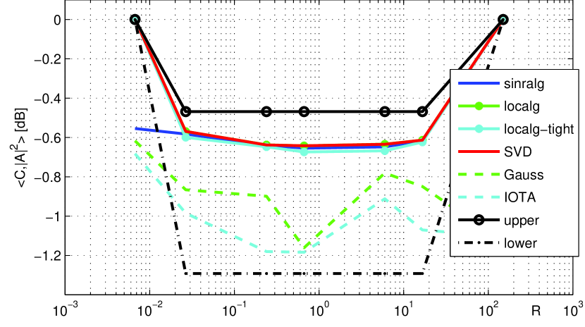
Figure 1: Localization $\langle\boldsymbol{C},|{\mathbf{A}}_{g\gamma}|^{2}\rangle$ for $|U|\approx 0.29$, lattice $|\Lambda|=1/2$ and OQAM signaling. $R$ has been varied.

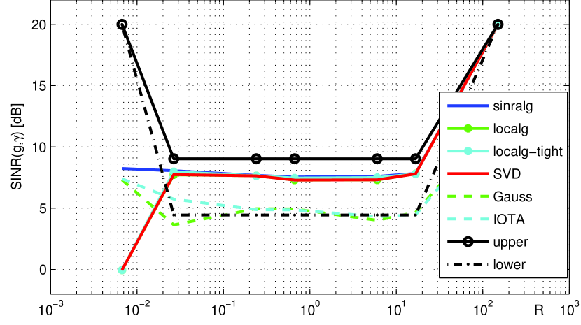
Figure 2: SINR for $|U|\approx 0.29$ at noise power $\sigma^{2}=-20$dB, lattice $|\Lambda|=1/2$ and OQAM signaling. $R$ has been varied.

Fig.1 shows the corresponding localization (9) and Fig.2 the SINR. It can be seen that the bounds are suited to describe the averaged performance of a multicarrier system in doubly–dispersive channels based only the support parameter $|U|$. It is interesting that also lower bound gives a quite useful estimate on the performance which is due to the uncritical condition number of $O$ at lattice density $|\Lambda|^{-1}=2$. For OFDM systems operating at ”more critical” lattices much more loss to the BLT has to be expected. The inner values of $R$ correspond to ”full” doubly–dispersive channels where no common eigenstructure can exists such that each decomposition is always an approximation. The boundary values in turn are single–dispersive channels having a joint exact eigenstructure, i.e. it is possible to completely suppress interference.

VI Conclusions

We have introduced the theory of pulse shaping with focus on the WSSUS–averaged SINR and considered the question of approximate eigenstructure of time–varying channels with compactly supported spreading. With increasing demand on bandwidth and efficiency the understanding of the fundamental limits in both directions will be important for future wireless communication systems. For Weyl–Heisenberg signaling, as a general description of OFDM and OFDM/OQAM communication systems, we found that both are on the level of localization equivalent. We have shown that simple localization bounds can be used to obtain general estimates on the eigenpair approximation behavior $E_{2}$ and the SINR itself. With the latter, for example, we are able to show fundamental limits on achievable performance based on simple statistical properties of the time–varying environment.

References

- [1] W. Kozek and A. Molisch, “On the eigenstructure of underspread WSSUS channels,” First IEEE Workshop on Signal Processing Advances in Wireless Communications, Paris, France, pp. 325–328, Apr 1997.
- [2] G. Matz and F. Hlawatsch, “Time-frequency characterization of random time-varying channels,” in Time-Frequency Signal Analysis and Processing: A Comprehensive Reference, B. Boashash, Ed. Oxford (UK): Elsevier, 2003, ch. 9.5, pp. 410–419.
- [3] W. Kozek, “Matched Weyl-Heisenberg expansions of nonstationary environments,” PhD thesis, Vienna University of Technology, 1996.
- [4] P. Jung and G. Wunder, “The WSSUS Pulse Design Problem in Multicarrier Transmission,” IEEE Trans. on. Communications, vol. 55, no. 10, pp. 1918–1928, Oct 2007. [Online]. Available: http://arxiv.org/abs/cs.IT/0509079
- [5] P. Jung, “Weighted Norms of Cross Ambiguity Functions and Wigner Distributions,” The 2006 IEEE International Symposium on Information Theory, 2006. [Online]. Available: http://arxiv.org/abs/cs.IT/0601017
- [6] G. B. Folland, Harmonic Analysis in Phase Space, ser. Annals of Mathematics Studies. Princeton University Press, 1989, no. 122.
- [7] P. Jung, “On the Approximate Eigenstructure of Time–Varying Channels,” submitted, 2008. [Online]. Available: http://arxiv.org/abs/0803.0610
- [8] G. Durisi, H. Bölcskei, and S. Shamai (Shitz), “Capacity of underspread WSSUS fading channels in the wideband regime,” in Proc. IEEE Int. Symposium on Information Theory (ISIT), July 2006, pp. 1500–1504. [Online]. Available: http://www.nari.ee.ethz.ch/commth/pubs/p/dbs˙isit06
- [9] J. Kohn and L. Nirenberg, “An algebra of pseudo-differential operators,” Communications on Pure and Applied Mathematics, vol. 18, no. 1-2, pp. 269–305, 1965.
- [10] G. Matz, “A Time-Frequency Calculus for Time-Varying Systems and Nonstationary Processes with Applications,” Ph.D. dissertation, Vienna University of Technology, Nov 2000.
- [11] P. Bello, “Characterization of randomly time–variant linear channels,” Trans. on Communications, vol. 11, no. 4, pp. 360–393, Dec 1963.
- [12] H. Feichtinger, “Modulation spaces on locally compact abelian groups,” University of Vienna, Tech. Rep., 1983.
- [13] P. Jung, “Weyl–Heisenberg Representations in Communication Theory,” Ph.D. dissertation, Technical University Berlin, 2007. [Online]. Available: http://opus.kobv.de/tuberlin/volltexte/2007/1619
- [14] T. Strohmer and S. Beaver, “Optimal OFDM Design for Time-Frequency Dispersive Channels,” IEEE Trans. on Communications, vol. 51, no. 7, pp. 1111–1122, Jul 2003.
- [15] P. Jung and G. Wunder, “On Time-Variant Distortions in Multicarrier with Application to Frequency Offsets and Phase Noise,” IEEE Trans. on Communications, vol. 53, no. 9, pp. 1561–1570, Sep 2005.
- [16] R. Chang, “Synthesis of Band-Limited Orthogonal signals for Multicarrier Data Transmission,” Bell. Syst. Tech. J., vol. 45, pp. 1775–1796, Dec 1966.
- [17] H. Bölcskei, “Orthogonal frequency division multiplexing based on offset qam,” in Advances in Gabor Theory, H. G. Feichtinger and T. Strohmer, Eds. Birkhäuser, 2003, ch. Orthogonal frequency division multiplexing based on offset QAM, pp. 321–352. [Online]. Available: http://www.nari.ee.ethz.ch/commth/pubs/p/gabor˙book˙chap
- [18] I. Daubechies, S. Jaffard, and J. Journé, “A simple Wilson orthonormal basis with exponential decay,” SIAM J. Math. Anal., vol. 22, no. 2, pp. 554–572, 1991.
- [19] A. Ron and Z. Shen, “Weyl–Heisenberg frames and Riesz bases in ,” Duke Math. J., vol. 89, no. 2, pp. 237–282, 1997.
- [20] A. Janssen and H. Boelcskei, “Equivalence of Two Methods for Constructing Tight Gabor Frames,” IEEE Signal Processing Letters, vol. 7, no. 4, p. 79, Apr 2000.
- [21] B. L. Floch, M. Alard, and C. Berrou, “Coded orthogonal frequency division multiplex,” Proceedings of the IEEE, vol. 83, pp. 982–996, Jun 1995.
- [22] K. Gröchenig, Foundations of Time–Frequency Analysis. Birkhäuser, 2001.
- [23] K. Gröchenig and M. Leinert, “Wiener’s lemma for twisted convolution and Gabor frames,” J. Amer. Math. Soc., vol. 17, pp. 1–18, 2003.
- [24] I. Daubechies, “Time–Frequency Localization Operators: A Geometric Phase Space Approach,” IEEE Transaction on Information Theory, vol. 34, no. 4, pp. 605–612, 1988.
- [25] K. Liu, T. Kadous, and A. M. Sayeed, “Orthogonal Time-Frequency Signaling over Doubly Dispersive Channels,” IEEE Trans. Info. Theory, vol. 50, no. 11, pp. 2583–2603, Nov 2004.