Cold quark stars from hot lattice QCD

Abstract

Based on a quasiparticle model for $\beta$ stable and electrically neutral deconfined matter we address the mass-radius relation of pure quark stars. The model is adjusted to recent hot lattice QCD results for 2 + 1 flavors with almost physical quark masses. We find rather small radii and masses of equilibrium configurations composed of cold deconfined matter, well distinguished from neutron or hybrid stars.

I Introduction

After growing evidence for the quark-gluon substructure of hadrons the question has been asked Ito70 ; Bay76 ; Kei76 ; Fre78 ; Fec78 whether massive neutron stars may have a core composed of quarks (Gle97, ; *Gle00; Web99, ; *Web05). These so-called hybrid stars may be part of the neutron star branch or constitute a separate stable branch of high-density objects – the so-called third family (Ger68, ; Kam81a, ; *Kam81b; *Kam83; *Kam85) or twin stars ScB02 . Also pure quark stars populating another separate branch of stable, spherically symmetric cold objects have been discussed Fec78 ; Ana79 ; Pes00 . All these possibilities depend sensitively on the equation of state at high density and the details of the deconfinement transition at low temperature. While at high temperature and zero net baryon density a proper numerical evaluation of the equation state based on first-principles – QCD – is accomplished, the knowledge of the equation of state at high baryon density and low temperature is fairly poor. In the asymptotic region, safe statements on the matter states can be made (Ris01, ; Raj01, ; *SW99), but the extrapolation to the interesting region of energy densities around $10^{15}$ g/cm³ is hampered by serious uncertainties as one expects significant non-perturbative effects.

A possibility to approach the theoretical analysis of quark stars is to employ certain models adjusted to high-temperature lattice QCD results at zero or small net baryon density. Of course, the applicability of such models at low temperatures and high densities is not guaranteed. Quarks stars or neutron stars with quark cores are expected to have similar mass-radius relations as ordinary neutron stars. This makes difficult an experimental verification via these observables. The modified cooling behavior of quark matter is considered as a possible tool to find appropriate observational hints Bla00 .

Here we are interested in the mass-radius relation of pure quark stars which are cold and spherically symmetric. We rely on a quasiparticle model (cf. (Pes94, ; *Pes96; SW01, ; *TSW04; Gar09, ) for such models) which we adjust to recent realistic lattice QCD results. Our quasiparticle model Pes94 ; BKS07a ; Sch08 allows for a suitable parametrization of lattice QCD data at zero and non-zero chemical potential. Its structure can be derived from a two-loop $\Phi$ functional Pes98a ; BIR01 ; Sch09 . To accommodate further non-perturbative effects the running coupling $g_{s}$ is replaced by an effective coupling $G$. In the simplest version the imaginary parts of the self-energies are neglected and the dispersion relation is approximated by utilizing the asymptotic self-energy. The model has been shown to describe successfully various lattice QCD data at zero chemical potential, at non-zero (including also purely imaginary) chemical potential of bulk thermodynamical quantities up to off-diagonal susceptibilities Blu04b ; Blu08a ; Blu08b .

New high-temperature lattice QCD data for almost physical quark masses Che07 ; Baz09 are now at our disposal for zero chemical potential. We adjust our model at this data and extrapolate the equation of state to zero temperature. The emerging equation of state is then used to consider cold pure quark stars. Analog studies have been performed in, e.g., (Pes01b, ; *Pes03; Iva05, ; Fra01, ; *Fra02; AS02, ; SLS99, ), however without such intimate contact to advanced lattice QCD results.

Our paper is organized as follows. In section II we formulate our model for zero temperature. The comparison with hot lattice QCD results is performed in section III. The parameters are used in section IV to gain the cold equation of state. The emerging mass-radius relations of cold equilibrium configurations are discussed in section V. The summary can be found in section VI. The Appendix lists expressions used for transferring the hot lattice QCD data to finite baryon densities.

II Quasiparticle model at $\boldsymbol{T=0}$

For the employed quasiparticle model the pressure $p=\sum_{i=u,d,s}p_{i}$ and quark densities $n_{i}$ at temperature $T=0$ are given by

$$p_{i}(\mu_{i}) = \frac{d_{i}}{6\pi^{2}}\int_{0}^{\sqrt{\mu_{i}^{2}-m_{i}^{2}}}dk\frac{k^{4}}{\sqrt{k^{2}+m_{i}^{2}}}-B_{i}(\mu_{i}),$$ (1)

$$B_{i}(\mu_{i}) = B_{i}(\mu_{0})+\frac{d_{i}}{4\pi^{2}}\int_{\mu_{0}}^{\mu_{i}}d\bar{\mu}\,\frac{\partial m_{i}^{2}(\bar{\mu})}{\partial\bar{\mu}}\int_{0}^{\sqrt{\bar{\mu}^{2}-m_{i}^{2}}}dk\frac{k^{2}}{\sqrt{k^{2}+m_{i}^{2}}},$$ (2)

$$n_{i}(\mu) = \frac{d_{i}}{6\pi^{2}}(\mu_{i}^{2}-m_{i}^{2})^{3/2}$$ (3)

with the index $i$ denoting the quarks $u$, $d$ and $s$ with degeneracies $d_{u,d,s}=2N_{c}=6$. The choice of $\mu_{0}$ and the corresponding integration constant $B(\mu_{0})$ is described below. The energy density follows from $e=\sum_{i=u,d,s}(p_{i}+\mu_{i}n_{i})$. The asymptotic quark masses, which enter the employed dispersion relations $\omega_{i}^{2}=k^{2}+m_{i}^{2}$ as approximation of the self-energies, are

$$m_{i}^{2} = m_{i,0}^{2}+2m_{i,0}M_{i}+2M_{i}^{2},$$ (4)

$$M_{i}^{2} = \frac{C_{\text{f}}}{8}\left(T^{2}+\frac{\mu_{i}^{2}}{\pi^{2}}\right)G^{2}$$ (5)

with $C_{\text{f}}=(N_{c}^{2}-1)/(2N_{c})$, where the rest masses $m_{i,0}$ may be included accordingly. We employ $m_{u,0}=m_{d,0}=m_{s,0}/10$ with $m_{s,0}$ = 105 MeV as in Baz09 ; Che07 . For later use also the temperature dependence is displayed here and we note already the gluon $g$ asymptotic mass at finite temperature

$$m_{g}^{2}=\left(\negmedspace\frac{C_{\text{b}}}{6}T^{2}+\frac{N_{c}}{12\pi^{2}}\sum_{i=u,d,s}\mu_{i}^{2}\right)G^{2},$$ (6)

where $C_{\text{b}}=N_{c}+\frac{3}{2}$ and the degeneracy factor $d_{g}=N_{c}^{2}-1$.

The five relations for charge neutrality

$$\frac{2}{3}n_{u}(\mu_{u})-\frac{1}{3}n_{d}(\mu_{d})-\frac{1}{3}n_{s}(\mu_{s})-n_{e}(\mu_{e})-n_{\mu}(\mu_{\mu})=0,$$ (7)

for $\beta$ equilibrium

$$\mu_{d}=\mu_{u}+\mu_{e}$$ (8)

(e.g., from $n\leftrightarrow p^{+}+e^{-}+\bar{\nu}_{e}$), for equilibrium due to strangeness changing weak decays

$$\mu_{s}=\mu_{d}$$ (9)

(e.g., from $\Lambda\leftrightarrow p^{+}+\pi^{-}$), for $\mu$ decay

$$\mu_{\mu}=\mu_{e}$$ (10)

(e.g., from $\mu^{-}\leftrightarrow e^{-}+\bar{\nu}_{e}+\nu_{\mu}$), and for total baryon density

$$n(\mu)=\frac{1}{3}(n_{u}(\mu_{u})+n_{d}(\mu_{d})+n_{s}(\mu_{s}))$$ (11)

map the various chemical potentials on one independent baryon chemical potential $\mu$ via $\mu_{u,d,s,e,\mu}(\mu)$ as required as consistency condition of the utilized quasiparticle model. We assume that the neutrinos $\nu_{e,\mu}$ left the star matter and, therefore, do not participate in the chemical equilibrium reactions. The pressure and density expressions for the electron $e$ and muon $\mu$ components are as Eqs. (1) (without the functions $B_{i}$) and (3).

The effective coupling $G^{2}$ follows from the flow equation Pes00 ; BKS07a

$$a_{T}\frac{\partial G^{2}(\mu,T)}{\partial T}+a_{\mu}\frac{\partial G^{2}(\mu,T)}{\partial\mu}=b,$$ (12)

where the coefficients $a_{T}$, $a_{\mu}$ and $b$ (cf. Appendix A) depend again on the effective coupling $G^{2}$ as well as both temperature and chemical potential. It is integrated using the method of characteristics. Along each characteristic line, the input information $G^{2}(T)$, extracted from lattice QCD data in the next section, is transported from the temperature axis to the chemical potential axis thus providing $G^{2}(\mu)$. Along one arbitrary characteristic, emerging at $T=T_{0}$ and meeting the $\mu$ axis at $\mu_{0}$, the meanfield contribution $B$ is integrated (as outlined in Appendix A too), yielding the necessary integration constant $B(\mu_{0})$. With the effective coupling $G^{2}(\mu)$ and the $B(\mu_{0})$, all thermodynamic quantities along $T=0$ are then determined.

III Equation of state from lattice QCD data at $\boldsymbol{\mu=0}$

In Baz09 (Che07 ) the interaction measure $\Delta(T)/T^{4}\equiv(e-3p)/T^{4}$ has been presented for almost physical quark masses for the two light quarks and a strange quark in the temperature range $T=140$ - 475 MeV (140 - 825 MeV) at $\mu_{i}=0$. We rely here on the p4 and asqtad data for $N_{\tau}=8$ Baz09 and 6 Che07 and assume that further cut-off effects are negligible, i.e. we compare our continuum model with the finite-size results Baz09 ; Che07 . It seems most appropriate to adjust our parameters directly at the interaction measure, being the primary information from lattice QCD, which reads in the quasiparticle model BKS07a for $\mu=0$

$$\frac{e-3p}{T^{4}} = \frac{1}{T^{4}}\sum_{i=g,u,d,s}\left(4B_{i}+\frac{d_{i}m_{i}^{2}}{\pi^{2}}\int_{0}^{\infty}dk\,k^{2}\frac{(k^{2}+m_{i}^{2})^{-1/2}}{e^{\sqrt{k^{2}+m_{i}^{2}}/T}+S_{i}}\right),$$ (13)

$$B_{i}(T) = B_{i,0}-\frac{d_{i}}{2\pi^{2}}\int_{T_{0}}^{T}dT^{\prime}\,\frac{\partial m_{i}^{2}(T^{\prime})}{\partial T^{\prime}}\int_{0}^{\infty}dk\,k^{2}\frac{(k^{2}+m_{i}(T^{\prime})^{2})^{-1/2}}{e^{\sqrt{k^{2}+m_{i}(T^{\prime})^{2}}/T^{\prime}}+S_{i}},$$ (14)

where $S_{g}=-1$ and $S_{u,d,s}=1$ and $m_{i}$ from Eqs. (4) and (6) with explicit and implicit $T$ dependencies. The latter one is in $G^{2}$ for which we choose

$$G^{2}(T)=\frac{16\pi^{2}}{\beta_{0}\ln\xi^{2}}$$ (15)

with $\xi\equiv\frac{T-T_{s}}{\lambda}$ as well as $\beta_{0}=11-\frac{2}{3}N_{f}$ for $N_{f}=2+1$ flavors as a convenient parametrization of the effective coupling which resembles a regularized 1-loop running coupling.

Using general thermodynamic relations one can calculate the pressure via $p(T)/T^{4}=p(T_{0})/T_{0}^{4}+\int_{T_{0}}^{T}dT^{\prime}\,\Delta(T^{\prime})\,T^{\prime-5}$, where $p(T_{0})$ is an integration constant. The chosen value of $T_{0}$ should be at the lower limit of our model for deconfinement, i.e. $T_{0}\approx 190$ MeV according to Baz09 . The scaled entropy density is accordingly $s/T^{3}=4p/T^{4}+\Delta/T^{4}$; unfortunately, it depends also on the pressure normalization via $4p(T_{0})/T_{0}^{4}$.

Our quasiparticle model is based primarily on the entropy density $s$, i.e. pressure and interaction measure are analytic integrals of the entropy including an integration constant $B_{0}=\sum B_{i,0}$. Thus fitting the interaction measure means not only determining the parameters $T_{s}$ and $\lambda$ of the effective coupling but also the pressure integration constant $B_{0}$. Thus, our pressure as well as entropy and energy density follow directly from $e-3p$ without another integration constant. (This is due to additional knowledge of explicit expressions for all thermodynamic quantities, as opposed to general thermodynamic relations, where an additional constant $p(T_{0})$ is required to arrive from the interaction measure at the pressure. Within the quasiparticle model, $p(T_{0})$ is known from the parameters $T_{s}$, $\lambda$ and $B_{0}$ via the expressions of $s$ and $\Delta$ in $p(T_{0})=(Ts(T_{0};T_{s},\lambda)-\Delta(T_{0};T_{s},\lambda,B_{0}))/4$.)

action	$N_{\tau}$	$T_{s}$ [MeV]	$\lambda$ [MeV]	$-B_{0}$	$\chi^{2}/$dof
p4	6	167	20	-(78 MeV)4	0.821
p4	8	146	31	(163 MeV)4	0.679
asqtad	6	131	45	(90 MeV)4	0.981 *)
asqtad	8	107	61	(166 MeV)4	0.654

Table 1: Parameters of fits to the lattice data Baz09 ; Che07 for $T>190$ MeV. $B_{0}=\sum_{i=g,u,d,s}B_{i,0}$.
*) Without the data point at 213 MeV which would drive the fit to fail in the high-temperature region.

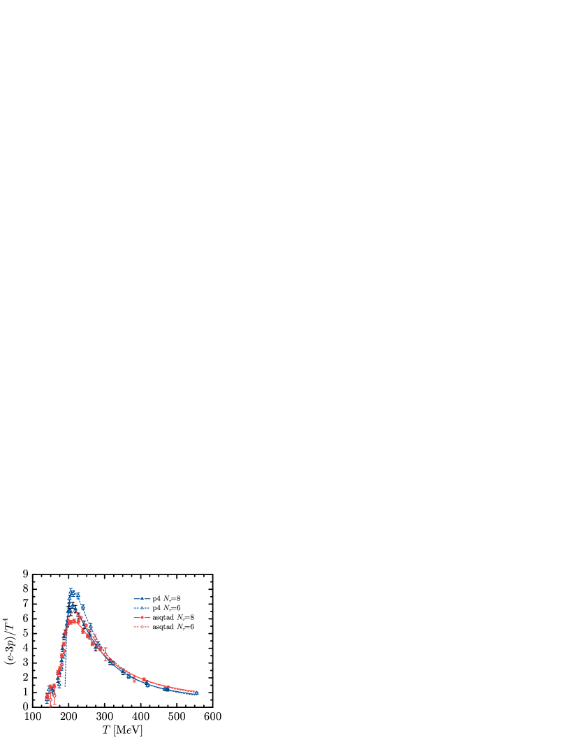
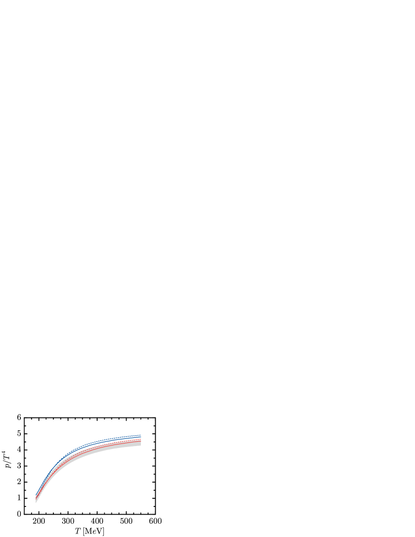
Figure 1: (color online) Left panel: Fits of the quasiparticle model interaction measure Eq. (13) to the lattice QCD data (symbols) for lattice actions p4 (blue) and asqtad (red) and lattice spacings $N_{\tau}$ from Baz09 ; Che07 . Solid (dashed) curves are for $N_{\tau}=8$ (6). Right panel: Scaled pressure $p/T^{4}$ of the quasiparticle model adjusted in the left panel compared to the pressure estimate from Baz09 (grey area).

The $\chi^{2}$ minimization of the difference of the data in Baz09 ; Che07 to the interaction measure Eq. (13) directly yields the values of $T_{s}$, $\lambda$ and $B_{0}$ as listed in Tab. 1. With this parametrization we get the interaction measure as exhibited in the left panel of Fig. 1. The maximum of $\Delta$ arises from a turning point of the scaled pressure as a function of $\log\,T$. Within our quasiparticle model, the location of the maximum is governed by the values of $T_{s}$ and $\lambda$, where the latter one also affects the peak width. The peak height of $\Delta/T^{4}$ is essentially determined by $B_{0}$. The fits are in a narrow corridor for $T$ > 300 MeV yielding some confidence in the equation of state there.

In the right panel of Fig. 1 we compare the pressure of our model with the pressure estimate deduced in Baz09 from the interaction measure. Despite of the variation of the peak heights in $\Delta/T^{4}$, the resulting pressures in our model are in a reasonably narrow corridor: Our fit to the asqtad $N_{\tau}=8$ data is in the middle of the pressure range determined in Baz09 by different interpolations on the data for $\Delta/T^{4}$ and assumptions on $p_{0}$. The p4 $N_{\tau}=6$ peak in $\Delta/T^{4}$ is higher, and, consequently, our pressure is also somewhat higher, governed by the positive $B_{0}$. A fit to the upper and lower limits of the pressure band from Baz09 would result in $(T_{s},\lambda,-B_{0})$ = (109 MeV, 53 MeV,(185 MeV)⁴) and (36 MeV, 107 MeV, (197 MeV)⁴), respectively.

IV The quark equation of state at zero temperature

Utilizing the values of Tab. 1 the flow equation (12) is solved using the mentioned method of characteristics to obtain $G^{2}(\mu)$ and $B(\mu)$. In doing so, the side conditions (7-11) are invoked so that along each characteristic curve the requirements of $\beta$ stability and electric charge neutrality are fulfilled. The characteristics for the p4 action and $N_{\tau}=8$ are exhibited in Fig. 2. As already noted in Pes00 ; BKS07a , the characteristics emerging from the very vicinity of $T_{0}$ have the tendency to cross each other at low temperatures. (An extended version of the model in Sch08 ; Sch08b cures this insanity.) The pressure becomes negative at $\mu<$ 550 MeV. Clearly, we consider only the region of positive pressure where the characteristics behave regularly.

Figure 2: Characteristics of the flow equation (12) with side conditions (7-11) imposed for the p4 action and $N_{\tau}=8$.

It happens that the effective coupling $G^{2}$ can also be parametrized at vanishing temperature using Eq. (15) but with $\xi\equiv\frac{\mu-\mu_{s}}{\lambda_{\mu}}$. The parameters are listed in Tab. 2. The interaction measure $\Delta(\mu)/\mu^{4}$ displays a peak, as $\Delta(T)/T^{4}$ does.

The pressure contributions according to Eq. (1) with the such obtained effective coupling $G^{2}(\mu)$ are exhibited in the left panel of Fig. 3 as a function of the chemical potential $\mu=\mu_{u}$. The differences of up, down and strange quark contributions are determined by differences in the respective chemical potentials as shown in the right panel of Fig. 3. Due to equilibrium with respect to strangeness changing weak decays, $\mu_{d}=\mu_{s}$ holds which deviates slightly from $\mu_{u}$. In line with SW99 the lepton contributions are tiny, as evidenced in Fig. 3, too. The pressure difference of down and strange quarks is due to the considerably larger rest mass of the latter ones. For the sake of completeness we also show the individual contributions to energy density (left panel in Fig. 4) and the individual particle densities (right panel in Fig. 4). Similar to the pressure, the lepton contributions are not visible on the used scales.

action	$N_{\tau}$	$\mu_{s}$ [MeV]	$\lambda_{\mu}$ [MeV]
p4	6	211	159
p4	8	134	215
asqtad	6	68	285
asqtad	8	-72	380

Table 2: Parameters of Eq. (15) with $\xi\equiv\frac{\mu-\mu_{s}}{\lambda_{\mu}}$ following from the solution of the flow equation Eq. (12). The fits apply in the range $\mu$ = 0.6…1.2 GeV.

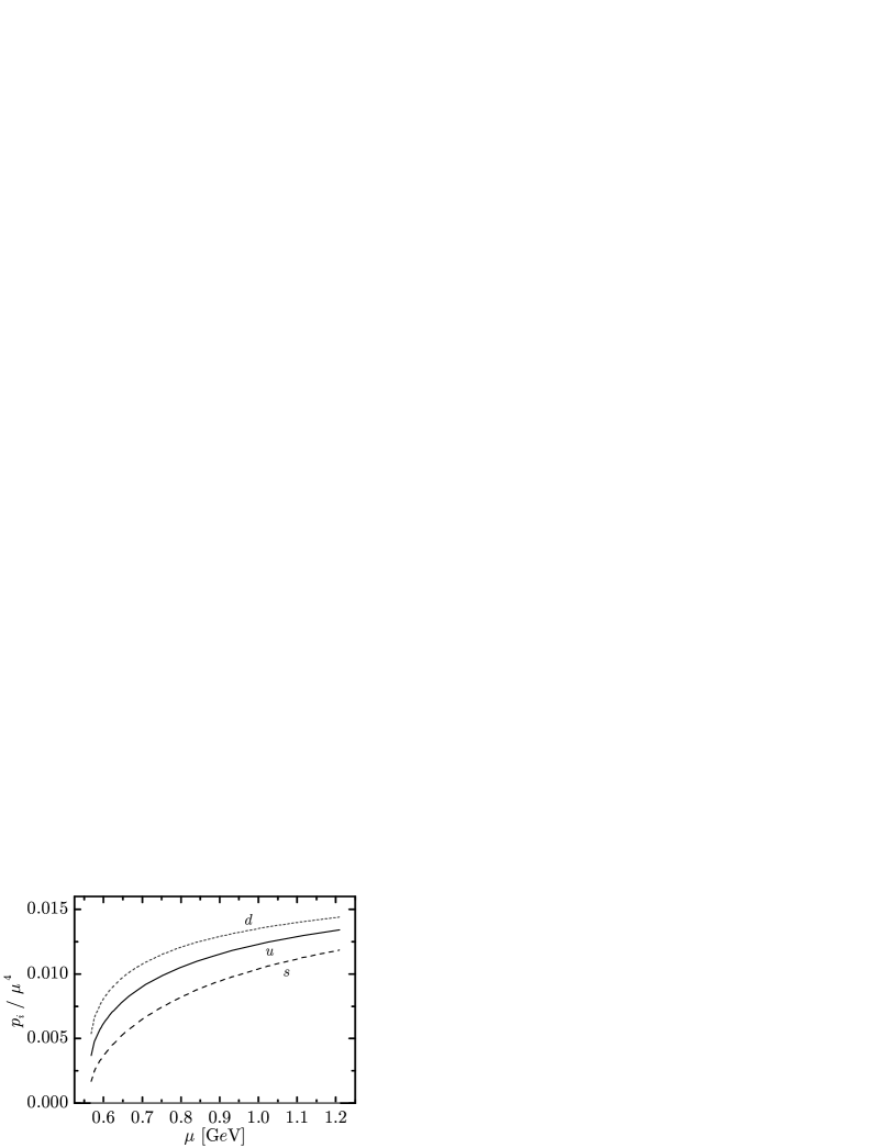
Figure 3: Left panel: The scaled pressure contributions $p_{i}/\mu^{4}$ for the p4 action and $N_{\tau}=8$ as functions of $\mu$. The leptonic contributions are on the lower $\mu$ axis in the given $p_{i}/\mu^{4}$ scale. Right panel: The individual chemical potentials $\mu_{i}$ as functions of $\mu=\mu_{u}$.

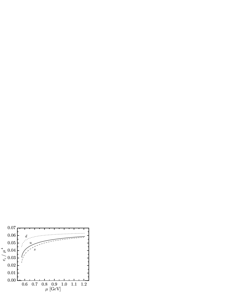
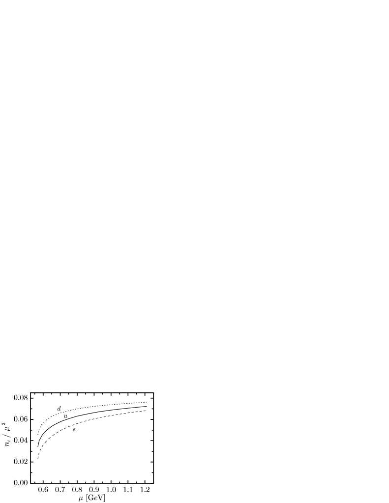
Figure 4: The scaled energy density contributions $e_{i}/\mu^{4}$ (left panel) and the scaled net quark density $n_{i}/\mu^{3}$ (right panel) for the p4 action and $N_{\tau}=8$ as functions of $\mu$. For the used scale, the leptonic contributions are not visible.

The resulting equation of state at $T=0$ in the form $e(p)$, needed for the integration of the TOV equations below, is exhibited in Fig. 5 (left panel for a comparison of the four equations of state) together with two fits by $e=v_{s}^{-2}p+e_{0}$ for the equations of state adjusted to $N_{\tau}=6$ and 8 for the p4 action (right panel). Parameters for all actions and temporal lattice extends considered here are listed in Tab. 3. Both, the vacuum energy density $e_{0}=e(p=0)$ and the velocity of sound parameter $v_{s}^{2}=\partial p/\partial e$ are in narrow intervals for the fours sets of lattice QCD input data: While the vacuum energy density varies within (366 MeV)⁴ - (381 MeV)⁴, $v_{s}^{-2}$ is within 3.8 - 4.5. As the interaction measure $\Delta(\mu)/\mu^{4}$ becomes small at large values of $\mu$, our resulting equations of state $e(p)$ have the tendency to merge. (Some differences are caused by the different fit values of $B_{0}$.) At small pressure the deviation of our four equations of state are about 10%.

The same is true if considering again the upper and lower limits of the pressure band from Baz09 instead of the interaction measure. We find values ($v_{s}^{-2},e_{0}^{1/4})$ = (3.92, 370 MeV) and (4.24, 383 MeV) in the parameter area of the above fits where larger values of the pressure at vanishing chemical potential lead to smaller values of the vacuum energy density at vanishing temperature and the inverse squared velocity of sound. Also, thermal effects are found to be small, i.e. up to $T=50$ MeV the equation of state $e(p)$ does not change significantly.

action	$N_{\tau}$	$v_{s}^{-2}$	$e_{0}^{1/4}$ [MeV]
p4	6	3.81	381
p4	8	4.01	366
asqtad	6	4.23	379
asqtad	8	4.47	367

Table 3: Parameters of linear fits $e=v_{s}^{-2}p+e_{0}$ to our equation of state with $G^{2}(\mu)$ determined by the flow equation (12). The leptonic contributions are included.

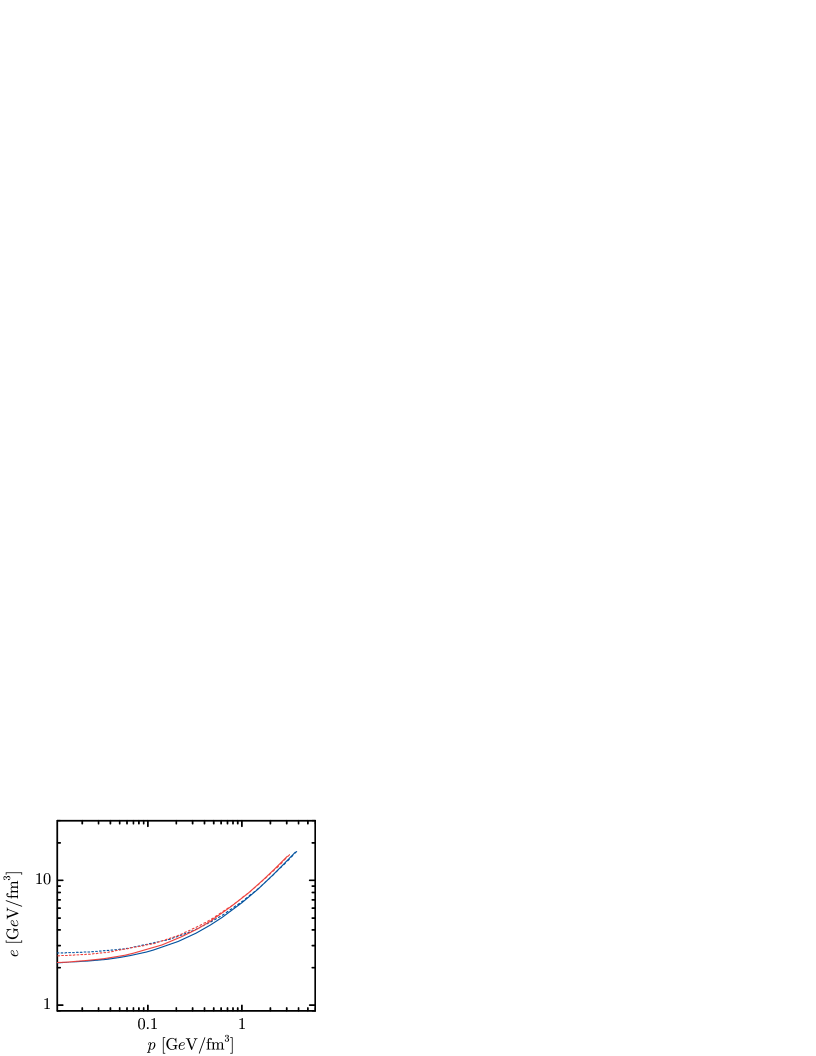
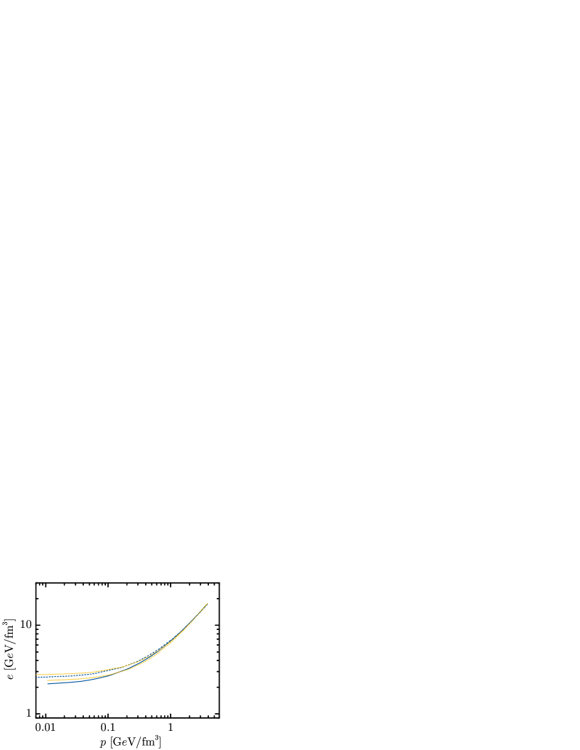
Figure 5: (color online) Left panel: The energy density as a function of the pressure at $T=0$ (solid curves) for all four considered lattice results from Baz09 ; Che07 . Blue (red) lines represent results deduced from p4 (asqtad) lattice data while solid (dashed) curves denote $N_{\tau}=8$ (6). Right panel: Two of the linear fits $e=v_{s}^{-2}p+e_{0}$ (dotted curves) from Tab. 3 compared to the corresponding equations of state (color code as in left panel).

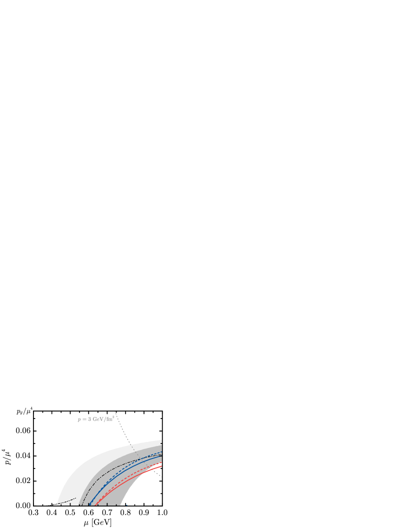
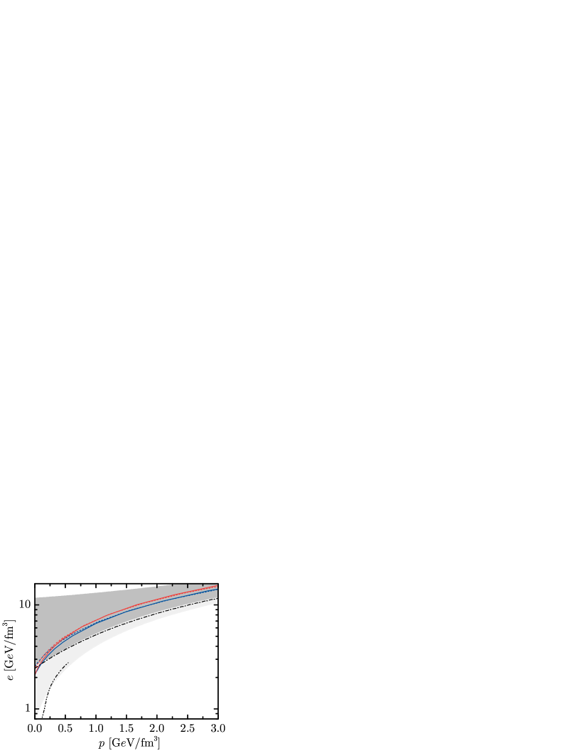
Figure 6: (color online) The scaled pressure $p/\mu^{4}$ as function of $\mu$ at $T=0$ (left panel) and the equation of state $e(p)$ (right panel) for the four considered lattice results from Baz09 ; Che07 in comparison to results from AS02 (dash-dotted curve), SLS99 (dash-double-dotted curve) and Fra01 ; Fra02 (grey bands limited by $\bar{\mu}/\mu$ = 1, 1.5 and 2 from dark to light). Blue (red) curves represent quasiparticle results adjusted to p4 (asqtad) lattice data while solid (dashed) curves denote $N_{\tau}=8$ (6). Leptonic contributions are included.

Our results can be compared with perturbative calculations at vanishing temperature in AS02 ; Fra01 ; Fra02 . In AS02 the pressure of cold quark matter is calculated in hard-dense-loop perturbation theory. The resulting pressure for 3 flavors with equal chemical potential and the choice AS02 of the renormalization scale $\bar{\mu}=\mu$ is shown in the left panel of Fig. 6. Also shown are the results from the weak-coupling expansion to second order Fra01 ; Fra02 . Here the value of $\bar{\mu}$ is varied from $\mu$ to 2$\mu$. For reference also a comparison with NJL model results SLS99 is depicted. The grey dotted curve is $p$ = 3 GeV/fm³; the region 0 < $p$ < 3 GeV/fm³ is relevant for quark stars, as turns out by integrating the TOV equations (see section V).

The energy density $e=\mu^{2}\partial/\partial\mu(p/\mu)$ depends on the incline of the pressure scaled with the chemical potential rather than the absolute values of the pressure. This explains the fact that, while the scaled quasiparticle pressure $p/\mu^{4}$ from lattice QCD (left panel in Fig. 6) shows some spread as a function of $\mu$, the resulting equation of state $e(p)$ (right panel in Fig. 6) is given as a tight band. Inspection of $p/\mu$ as a function of $\mu$ (not displayed) explains the broad range of values for $e(p\rightarrow 0)$ in Fra01 ; Fra02 : the slope of $p/\mu$ as a function of $\mu$ changes drastically with the chosen scale $\bar{\mu}$ for small pressures. For $\bar{\mu}$ = 1.5$\mu$ the equation of state in Fra01 ; Fra02 in the form $e(p)$ coincides with the results of AS02 , which in turn falls in the same range as our set of equations of state. In fact, $v_{s}^{-2}=3$ and $e_{0}^{1/4}$ = 365 MeV yield a good description of the equation of state from Fra01 ; Fra02 for $\bar{\mu}$ = 1.2$\mu$ and AS02 . (Expanding the quasiparticle partial pressure $p_{i}$ (1) including the meanfield contribution $B_{i}$ (2) at $T=0$ in powers of the coupling constant $G$ yields the leading terms $p_{i}(\mu_{i})=\left(1-2\alpha_{s}/\pi+\ldots\right)\mu_{i}^{4}/(4\pi^{2})+B_{i}(\mu_{0})$, where the coefficient of the $\mathcal{O}(\alpha_{s})$ term, $\alpha_{s}=4\pi G^{2}$, equals the strictly perturbative results in Fre77c ; Fra01 ; Fra02 ; the coefficient of the next-order term deviates from the perturbation expansion, similar to the quasiparticle model Pes00 ; Pes94 ; Pes96 (see also discussion in BIR01 ) at non-zero temperature and the hard-dense-loop approach in AS02 .)

Remarkable is that all the discussed equations of state have a certain value of the chemical potential at vanishing pressure. This enables, in principle, to construct pure quark stars with vanishing pressure at the surface.

Fig. 6 clearly evidences that the previous foundation for discussing quark stars seemed not to be on safe grounds as the proposed model equations of state were too different unless further constraints (as the compatibility, e.g., with a hadronic model equation of state required in Fra02 ) are imposed. Given the intimate contact of our approach to first-principle evaluations of QCD, we hope to have a more reliable foundation. Of course, this hope is related to the assumption that the extrapolation to non-zero chemical potential is sufficiently smooth. The successful comparison of our model with Taylor expansion coefficients for the $\mu$ dependence Blu04b as well as the application of our model at imaginary chemical potential Blu08a (not only small values thereof!) give us some confidence in our approach.

Let us finally comment on the importance of the side conditions. If one assumes one common chemical potential for all quarks $\mu$ and includes leptons ($\mu_{e}=\mu_{\mu})$ via a electric neutrality condition $\mu_{e}=\mu_{e}(\mu)$ , the results of the equation of state differ from the isospin asymmetric model with the side conditions (7-11) properly invoked on a 10% level.

V Integration of the TOV equations

To estimate the properties of quark stars as spherical equilibrium configurations of pure, strongly interacting quark matter we employ the TOV equations

$$\frac{dp}{dr} = -G_{N}\frac{([1+v_{s}^{-2}]p+e_{0})(m+4\pi r^{3}p)}{r^{2}(\,1-\frac{2m}{r}G_{N})},$$ (16)

$$\frac{dm}{dr} = 4\pi r^{2}(v_{s}^{-2}p+e_{0}),$$ (17)

where the special parametrization $e=v_{s}^{-2}p+e_{0}$ of the equation of state is supposed to hold. $G_{N}$ is the Newtonian gravitational constant, and we employ units with $\hbar c=1$.

We emphasize the strong dependence on the actual value of $e_{0}$ which determines the pressure gradient in the dimensionless combination $G_{N}e_{0}^{1/2}$ (which is of the order of 10^-39 for the case at hand), which can be seen in writing the TOV equations as

$$\frac{\partial\bar{p}}{\partial\bar{r}} = -\frac{\left(\left[1+v_{s}^{-2}\right]\bar{p}+1\right)\left(\bar{m}+4\pi\bar{r}^{3}\bar{p}\right)}{\bar{r}^{2}\left(1-\frac{2\bar{m}}{\bar{r}}\right)},$$ (18)

$$\frac{\partial\bar{m}}{\partial\bar{r}} = 4\pi\bar{r}^{2}\left(v_{s}^{-2}\bar{p}+1\right),$$ (19)

from the scaled quantities $p=\bar{p}e_{0}$, $r=\bar{r}(G_{N}e_{0})^{-1/2}$, $m=\bar{m}(G_{N}e_{0})^{-1/2}G_{N}^{-1}$. The scaled TOV equations depend only on $v_{s}^{-2}$. The solutions for the relevant values of $v_{s}^{-2}=$ 2…4 are exhibited in Fig. 7. With the given scaling, $m$ and $r$ shrink with increasing value of $e_{0}^{1/2}$, while the dependence on $v_{s}^{-2}$ is moderate within the interval covering the values of Tab. 3. Thus the vacuum energy density $e_{0}$ is indeed the decisive quantity determining the sizes and the masses of pure quark stars. To be specific, for $v_{s}^{-2}=3\pm 1$, the scaled maximum mass is 0.004 $\pm$ 0.001.

To test the dependence of deviations from the approximation $e=v_{s}^{-2}p+e_{0}$ we integrate the TOV equations with our equations of state adjusted to the lattice QCD results. The results are exhibited in Fig. 8. The maximum masses are about 0.5$M_{\odot}$ with radii of about 3 km. If such objects would exist, their bulk characteristics were quite different from canonical neutron stars with masses concentrated at 1.4 $M_{\odot}$ and radii of 15 km and larger. Therefore, the pure quark stars from our analysis cannot serve as candidates of twin stars discussed in ScB02 .

We stress again the important role of the value of $e_{0}=e(p=0)$. With the above derived scaling, equations of state with significantly smaller values of $e_{0}$ than deduced in our analysis of the lattice QCD results combined with the employed quasiparticle model, would allow for significantly larger masses and radii.

The present considerations will be modified when combining our equation of state of deconfined matter with a hadronic low-density equation of state at $p>0$. Then hybrid stars could be constructed with properties depending to a large extent on the transition region from confined to deconfined matter.

Figure 7: Scaled mass $\bar{M}=\bar{m}(p=0)$ shown as a function of scaled radius $\bar{R}=\bar{r}(p=0)$ for several values of $v_{s}^{-2}$ as solution of the scaled TOV equations (18) and (19).

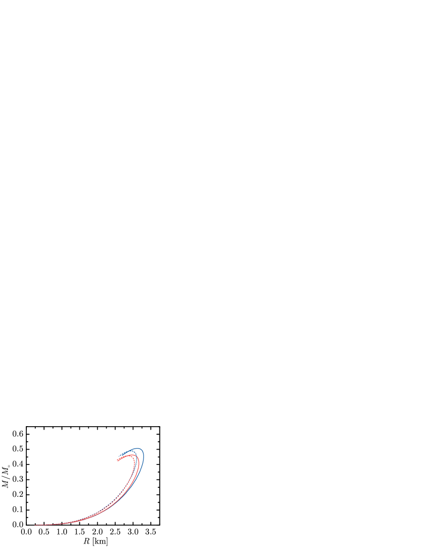
Figure 8: (color online) Mass-radius relations of quark stars following directly from lattice QCD results Baz09 ; Che07 within our quasiparticle approach. Blue (red) lines represent results deduced from p4 (asqtad) lattice data while solid (dashed) curves denote $N_{\tau}=8$ (6).

VI Summary

In summary we employ a quasiparticle model, adjusted to recent realistic lattice QCD data with almost physical quarks masses, to consider pure quark stars. The needed equation of state can be approximated very well by the concise form $e=v_{s}^{-2}p+e_{0}$ with values of $v_{s}^{-2}=3.8-4.5$ and $e_{0}^{1/4}=366-381$ MeV from the lattice QCD data Baz09 . Lattice data from both the p4 and the asqtad version can be described equally well and lead to similar spherically symmetric stars. The maximum masses are about 0.5 ${\rm M}_{\odot}$ with radii of 3 km.

The pure quarks star masses and radii scale with $e_{0}^{-1/2}$ which is the decisive quantity as $e_{0}$ is the vacuum energy density at vanishing pressure. It follows within our model directly from the lattice QCD data at finite temperatures.

Rapidly rotating quark stars exhibit a disc like shape with sharp edge. Their maximum masses are enlarged by 65% and the radii by a similar amount Ans03 at the shedding limit.

The present approach can be extended to the full HTL quasiparticle model Sch08 ; Sch09 , where effects of Landau damping and collective modes are included

Acknowledgments: The work is supported by BMBF 06DR9059D. Useful discussions with M. Bluhm, D. Blaschke, R. Meinel, D. Petrov and A. Teichmüller are gratefully acknowledged.

Appendix A Coefficients of the flow equation

The coefficients in Eq. (12) are

$$a_{T} = -\sum_{i=u,d,s}\frac{\partial n_{i}}{\partial m_{i}^{2}}\left.\frac{\partial m_{i}^{2}}{\partial G^{2}}\right|_{T,\mu},$$

$$a_{\mu} = \sum_{i=g,u,d,s}\frac{\partial s_{i}}{\partial m_{i}^{2}}\left.\frac{\partial m_{i}^{2}}{\partial G^{2}}\right|_{T,\mu},$$

$$b = \sum_{i=g,u,d,s}\frac{\partial n_{i}}{\partial m_{i}^{2}}\left.\frac{\partial m_{i}^{2}}{\partial T}\right|_{G^{2},\mu}-\frac{\partial s_{i}}{\partial m_{i}^{2}}\left.\frac{\partial m_{i}^{2}}{\partial\mu}\right|_{G^{2},T}$$

with

$$\frac{\partial n_{i}}{\partial m_{i}^{2}} = -\frac{d_{i}}{4\pi^{2}T}\int_{0}^{\infty}\!\mathrm{d}k\,\frac{k^{2}}{\omega_{i}}F_{-},$$

$$\frac{\partial s_{i}}{\partial m_{i}^{2}} = -\frac{d_{i}}{4\pi^{2}T}\int_{0}^{\infty}\!\mathrm{d}k\,k^{2}\left\{F_{+}-\frac{\mu_{i}}{\omega_{i}}F_{-}\right\},$$

where $F_{\pm}=\left[f_{+}^{2}\exp\frac{\omega_{i}-\mu_{i}}{T}\pm f_{-}^{2}\exp\frac{\omega_{i}+\mu_{i}}{T}\right]$ and $f_{\pm}$ are the statistical distribution functions for fermions (+) and anti-fermions (-) respectively. The derivatives of the effective gluon masses (6) are

$$\left.\frac{\partial m_{g}^{2}}{\partial T}\right|_{G^{2},\mu} = \frac{C_{\text{b}}}{3}TG^{2}+\frac{N_{c}}{12\pi^{2}}\left(N_{l}\!+\!2N_{h}\right)\left(\mu+\mu_{e}\right)\left.\frac{\partial\mu_{e}}{\partial T}\right|_{G^{2},\mu}G^{2},$$

$$\left.\frac{\partial m_{g}^{2}}{\partial\mu}\right|_{G^{2},T} = \frac{N_{c}}{12\pi^{2}}\left(\Big{(}2\left(N_{l}\!+\!N_{h}\right)\mu+\left(N_{l}\!+\!2N_{h}\right)\mu_{e}\Big{)}G^{2}+\left(N_{l}\!+\!2N_{h}\right)\left(\mu+\mu_{e}\right)\left.\frac{\partial\mu_{e}}{\partial\mu}\right|_{G^{2},T}\right),$$

$$\left.\frac{\partial m_{g}^{2}}{\partial G^{2}}\right|_{T,\mu} = \frac{C_{\text{b}}}{6}T^{2}+\frac{N_{c}}{12\pi^{2}}\left(N_{l}\!+\!2N_{h}\right)\left(\mu+\mu_{e}\right)\left.\frac{\partial\mu_{e}}{\partial G^{2}}\right|_{T,\mu}G^{2},$$

where $N_{l}$ and $N_{h}$ are the numbers of included light (2) and heavier (1) quark flavors. For the effective quark masses ($i=u,d,s$) one has

$$\left.\frac{\partial m_{i}^{2}}{\partial T}\right|_{G^{2},\mu}\!\!\! = \left.\frac{\partial m_{i}^{2}}{\partial T}\right|_{G^{2},\mu,\mu_{e}}\!\!\!+\left.\frac{\partial m_{i}^{2}}{\partial\mu_{e}}\right|_{G^{2},T,\mu}\left.\frac{\partial\mu_{e}}{\partial T}\right|_{G^{2},\mu},$$

$$\left.\frac{\partial m_{i}^{2}}{\partial\mu}\right|_{G^{2},T}\!\!\! = \left.\frac{\partial m_{i}^{2}}{\partial\mu}\right|_{G^{2},T,\mu_{e}}\!\!\!+\left.\frac{\partial m_{i}^{2}}{\partial\mu_{e}}\right|_{G^{2},T,\mu}\left.\frac{\partial\mu_{e}}{\partial\mu}\right|_{G^{2},T},$$

$$\left.\frac{\partial m_{i}^{2}}{\partial G^{2}}\right|_{T,\mu} = \left.\frac{\partial m_{i}^{2}}{\partial G^{2}}\right|_{T,\mu,\mu_{e}}+\left.\frac{\partial m_{i}^{2}}{\partial\mu_{e}}\right|_{G^{2},T,\mu}\!\left.\frac{\partial\mu_{e}}{\partial G^{2}}\right|_{T,\mu}$$

with $\left.\partial m_{i}^{2}/\partial T\right|_{G^{2},\mu,\mu_{e}}=VTG^{2}$, $\left.\partial m_{i}^{2}/\partial\mu\right|_{G^{2},T,\mu_{e}}=V\mu_{i}G^{2}/\pi^{2}$, $\left.\partial m_{i}^{2}/\partial\mu_{e}\right|_{G^{2},T,\mu}=\delta_{iu}V\mu_{i}G^{2}/\pi^{2}$ and $\left.\partial m_{i}^{2}/\partial G^{2}\right|_{T,\mu,\mu_{e}}=\left(T^{2}+\mu_{i}^{2}/\pi^{2}\right)/2$, where $V=\left(m_{q,0}/M_{q}+2\right)C_{\text{f}}/4$. The derivatives of the electron chemical potential therein are

$$\left.\frac{\partial\mu_{e}}{\partial T}\right|_{G^{2},\mu} = -W^{-1}\sum_{j=u,d,s,e,\mu}q_{j}\left.\frac{\partial n_{j}}{\partial T}\right|_{G^{2},\mu,\mu_{e}},$$

$$\left.\frac{\partial\mu_{e}}{\partial\mu}\right|_{G^{2},T} = -W^{-1}\sum_{j=u,d,s,e,\mu}q_{j}\left.\frac{\partial n_{j}}{\partial\mu}\right|_{G^{2},T,\mu_{e}},$$

$$\left.\frac{\partial\mu_{e}}{\partial G^{2}}\right|_{T,\mu} = -W^{-1}\sum_{j=u,d,s,e,\mu}q_{j}\left.\frac{\partial n_{j}}{\partial G^{2}}\right|_{T,\mu,\mu_{e}}$$

with $W=\sum_{j=u,d,s,e,\mu}q_{j}\left.\partial n_{j}/\partial\mu_{e}\right|_{G^{2},\mu,T}$ and

$$\left.\frac{\partial n_{i}}{\partial T}\right|_{G^{2},\mu,\mu_{e}} = \left.\frac{\partial n_{i}}{\partial T}\right|_{G^{2},\mu,\mu_{e},m_{i}^{2}}+\frac{\partial n_{i}}{\partial m_{i}^{2}}\left.\frac{\partial m_{i}^{2}}{\partial T}\right|_{G^{2},\mu,\mu_{e}},$$

$$\left.\frac{\partial n_{i}}{\partial\mu}\right|_{G^{2},T,\mu_{e}} = \left(\left.\frac{\partial n_{i}}{\partial\mu_{i}}\right|_{G^{2},m_{i}^{2}}+\frac{\partial n_{i}}{\partial m_{i}^{2}}\left.\frac{\partial m_{i}^{2}}{\partial\mu_{i}}\right|_{G^{2},T,\mu_{e}}\right)\left.\frac{\partial\mu_{i}}{\partial\mu}\right|_{\mu_{e}},$$

$$\left.\frac{\partial n_{i}}{\partial\mu_{e}}\right|_{G^{2},\mu,T} = \left(\left.\frac{\partial n_{i}}{\partial\mu_{i}}\right|_{G^{2},m_{i}^{2}}+\frac{\partial n_{i}}{\partial m_{i}^{2}}\left.\frac{\partial m_{i}^{2}}{\partial\mu_{i}}\right|_{G^{2},\mu}\right)\left.\frac{\partial\mu_{i}}{\partial\mu_{e}}\right|_{\mu},$$

$$\left.\frac{\partial n_{i}}{\partial G^{2}}\right|_{T,\mu,\mu_{e}} = \frac{\partial n_{i}}{\partial m_{i}^{2}}\left.\frac{\partial m_{i}^{2}}{\partial G^{2}}\right|_{T,\mu,\mu_{e}}$$

as well as

$$\left.\frac{\partial n_{i}}{\partial T}\right|_{G^{2},\mu,\mu_{e},m_{i}^{2}}\!\!\!\!\! = \frac{d_{i}}{2\pi^{2}T}\int_{0}^{\infty}\!\!\!\mathrm{d}k\,k^{2}\left\{\omega_{i}F_{-}-\mu_{i}F_{+}\right\},$$

$$\left.\frac{\partial n_{i}}{\partial\mu_{i}}\right|_{G^{2},m_{i}^{2}} = \frac{d_{i}}{2\pi^{2}T}\int_{0}^{\infty}\!\mathrm{d}k\,k^{2}F_{+}.$$

$q_{i}$ are the electric charges of the quark species. Note that the side conditions Eqs. (7-11) are included. These strongly modify the coefficients given in BKS07a .

Along the characteristics, where $\mu$, $T$ and $G^{2}$ are given as functions of the affine curve parameter $x$, the bag pressure $B$ has to be integrated according to

$$B=B(\mu=0)-\sum_{i}\int_{0}^{x}\text{d}x\frac{\partial p_{i}}{\partial m_{i}^{2}}\left(a_{T}\left.\frac{\partial m_{i}^{2}}{\partial T}\right|_{G^{2},\mu}+a_{\mu}\left.\frac{\partial m_{i}^{2}}{\partial\mu}\right|_{G^{2},T}+b\left.\frac{\partial m_{i}^{2}}{\partial G^{2}}\right|_{T,\mu}\right)$$

with

$$\frac{\partial p_{i}}{\partial m_{i}^{2}}=-\frac{d_{i}}{4\pi^{2}}\int_{0}^{\infty}\!\mathrm{d}k\,\frac{k^{2}}{\omega_{i}}\left[f_{+}+f_{-}\right].$$

References

- (1) N. Itoh, Prog. Theor. Phys. 44, 291 (1970)
- (2) G. Baym and S. A. Chin, Phys. Lett. B 62, 241 (1976)
- (3) B. D. Keister and L. S. Kisslinger, Phys. Lett. B 64, 117 (1976)
- (4) B. Freedman and L. McLerran, Phys. Rev. D 17, 1109 (1978)
- (5) W. B. Fechner and P. C. Joss, Nature 274, 347 (1978)
- (6) N. K. Glendenning, S. Pei, and F. Weber, Phys. Rev. Lett. 79, 1603 (1997), astro-ph/9705235
- (7) N. K. Glendenning, Compact stars: nuclear physics, particle physics, and general relativity (Springer, 2000) ISBN 0387989773
- (8) F. Weber, Pulsars as astrophysical laboratories for nuclear and particle physics (CRC Press, 1999) ISBN 0750303328
- (9) F. Weber, Prog. Part. Nucl. Phys. 54, 193 (2005), astro-ph/0407155
- (10) U. H. Gerlach, Phys. Rev. 172, 1325 (1968)
- (11) B. Kämpfer, J. Phys. A 14, L471 (1981)
- (12) B. Kämpfer, Phys. Lett. B 101, 366 (1981)
- (13) B. Kämpfer, J. Phys. G 9, 1487 (1983)
- (14) B. Kämpfer, Phys. Lett. B 153, 121 (1985)
- (15) J. Schaffner-Bielich, M. Hanauske, H. Stöcker, and W. Greiner, Phys. Rev. Lett. 89, 171101 (2002)
- (16) J. D. Anand, P. P. Bhattacharjee, and S. N. Biswas, J. Phys. A 12, L347 (1979)
- (17) A. Peshier, B. Kämpfer, and G. Soff, Phys. Rev. C 61, 045203 (2000), hep-ph/9911474
- (18) D. H. Rischke, D. T. Son, and M. A. Stephanov, Phys. Rev. Lett. 87, 062001 (2001), hep-ph/0011379
- (19) K. Rajagopal and F. Wilczek, Phys. Rev. Lett. 86, 3492 (2001), hep-ph/0012039
- (20) T. Schäfer and F. Wilczek, Phys. Rev. Lett. 82, 3956 (1999), hep-ph/9811473
- (21) D. Blaschke, T. Klähn, and D. N. Voskresensky, Astrophys. J. 533, 406 (2000)
- (22) A. Peshier, B. Kämpfer, O. P. Pavlenko, and G. Soff, Phys. Lett. B 337, 235 (1994)
- (23) A. Peshier, B. Kämpfer, O. P. Pavlenko, and G. Soff, Phys. Rev. D 54, 2399 (1996)
- (24) R. A. Schneider and W. Weise, Phys. Rev. C 64, 055201 (2001), hep-ph/0105242
- (25) M. A. Thaler, R. A. Schneider, and W. Weise, Phys. Rev. C 69, 035210 (2004), hep-ph/0310251
- (26) F. Gardim and F. Steffens, Nuclear Physics A 825, 222 (2009), arXiv:0905.0667
- (27) M. Bluhm, B. Kämpfer, R. Schulze, and D. Seipt, Eur. Phys. J. C 49, 205 (2007), hep-ph/0608053
- (28) R. Schulze, M. Bluhm, and B. Kämpfer, Eur. Phys. J. ST 155, 177 (2008), arXiv:0709.2262
- (29) A. Peshier, B. Kämpfer, O. P. Pavlenko, and G. Soff, Europhys. Lett. 43, 381 (1998)
- (30) J.-P. Blaizot, E. Iancu, and A. Rebhan, Phys. Rev. D 63, 065003 (2001), hep-ph/0005003
- (31) R. Schulze and B. Kämpfer, Prog. Part. Nucl. Phys. 62, 386 (2009), arXiv:0811.0274
- (32) M. Bluhm, B. Kämpfer, and G. Soff, Phys. Lett. B 620, 131 (2005), hep-ph/0411106
- (33) M. Bluhm and B. Kämpfer, Phys. Rev. D 77, 034004 (2008), arXiv:0711.0590
- (34) M. Bluhm and B. Kämpfer, Phys. Rev. D 77, 114016 (2008), arXiv:0801.4147
- (35) M. Cheng et al., Phys. Rev. D 77, 014511 (2008), arXiv:0710.0354
- (36) A. Bazavov et al., Phys. Rev. D 80, 014504 (2009), arXiv:0903.4379
- (37) A. Peshier, B. Kämpfer, and G. Soff(2001), hep-ph/0106090
- (38) A. Peshier, B. Kämpfer, and G. Soff, in Erevan 2003: Superdense QCD matter and compact stars, edited by D. Blaschke and D. Sedrakian (Springer, 2006) pp. 135–146, hep-ph/0312080
- (39) Y. B. Ivanov, A. S. Khvorostukhin, E. E. Kolomeitsev, V. V. Skokov, V. D. Toneev, and D. N. Voskresensky, Phys. Rev. C 72, 025804 (2005), astro-ph/0501254v2
- (40) E. S. Fraga, R. D. Pisarski, and J. Schaffner-Bielich, Phys. Rev. D 63, 121702 (2001), hep-ph/0101143
- (41) E. S. Fraga, R. D. Pisarski, and J. Schaffner-Bielich, Nucl. Phys. A 702, 217 (2002), nucl-th/0110077
- (42) J. O. Andersen and M. Strickland, Phys. Rev. D 66, 105001 (2002), hep-ph/0206196
- (43) K. Schertler, S. Leupold, and J. Schaffner-Bielich, Phys. Rev. C 60, 025801 (1999), astro-ph/9901152
- (44) R. Schulze, M. Bluhm, and B. Kämpfer, in XLVI International Winter Meeting on Nuclear Physics, Bormio (Italy), edited by I. Iori and A. Tarantola (University of Milan, 2008) p. 63, arXiv:0803.1571
- (45) B. A. Freedman and L. D. McLerran, Phys. Rev. D 16, 1169 (1977)
- (46) M. Ansorg, A. Kleinwächter, and R. Meinel, Astron.Astrophys. 405, 711 (2003), astro-ph/0301173