Uncertainty relation on world crystal and its applications to micro black holes

Abstract

We formulate generalized uncertainty relations in a crystal-like universe whose lattice spacing is of the order of Planck length — “world crystal”. In the particular case when energies lie near the border of the Brillouin zone, i.e., for Planckian energies, the uncertainty relation for position and momenta does not pose any lower bound on involved uncertainties. We apply our results to micro black holes physics, where we derive a new mass-temperature relation for Schwarzschild micro black holes. In contrast to standard results based on Heisenberg and stringy uncertainty relations, our mass-temperature formula predicts both a finite Hawking’s temperature and a zero rest-mass remnant at the end of the micro black hole evaporation. We also briefly mention some connections of the world crystal paradigm with ’t Hooft’s quantization and double special relativity.

PACS numbers: 04.70.Dy, 03.65.-w

I Introduction

Recent advances in gravitational and quantum physics indicate that in order to reconcile the two fields with each other, a dramatic conceptual shift is required in our understanding of spacetime. In particular, the notion of spacetime as a continuum may need revision at scales where gravitational and electro-weak interactions become comparable in strength Witten:96 . For this reason there has been a recent revival of interest in approximating the spacetime with discrete coarse-grained structures at small, typically Planckian, length scales. Such structures are inherent in many models of quantum-gravity, such as spacetime foam garay:98 , loop quantum gravity rovelli:04 ; gambini:99 ; alfaro:00 , non-commutative geometry camelia:00 ; susskind:00 ; camelia:01 ; douglas:01 , black-hole physics jacobson:08 or cosmic cellular automata Toffoli ; Wolfram1 ; Wolfram2 ; thooft1 ; thooft2 .

Despite a vast gap between the Planck length ($\ell_{p}\approx 1.6\cdot 10^{-35}$ m) and smallest length scales that can be probed with particle accelerators ($\approx 10^{-18}$ m), the issue of Planckian physics might not be so speculative as it seems. In fact, probes such as Planck Surveyor PS or the related IceCube IC — which just started or are planned to start in the near future, are supposed to set various important limits on prospective models of the Planckian world.

One of the simplest toy-model systems for Planckian physics is undoubtedly a discrete lattice. Discrete lattices are routinely used, for instance, in computational quantum field theory Creutz:83 ; Klein1 ; FIRST , but with a few notable exceptions Friedberg:83a ; Friedberg:83b ; MVF , they mainly serve as numerical regulators of ultraviolet divergences. Indeed, a major point of renormalized theories is precisely to extract lattice-independent data from numerical computations. One may, however, investigate the consequences of taking the lattice no longer as a mere computational device, but as a bona-fide discrete network, whose links define the only possible propagation directions for signals carrying the interactions between fields sitting on the nodes of the network.

Recently one of us proposed a model of a discrete, crystal-like universe — “world crystal” FIRST ; MVF ; rema0 . There, the geometry of Einstein and Einstein-Cartan spaces can be considered as being a manifestation of the defect structure of a crystal whose lattice spacing is of the order of $\ell_{p}$. Curvature is due to rotational defects, torsion due to translational defects. The elastic deformations do not alter the defect structure, i.e., the geometry is invariant under elastic deformations. If one assumes these to be controlled by a second-gradient elastic action, the forces between local rotational defects, i.e., between curvature singularities, are the same as in Einstein’s theory ANN . Moreover, the elastic fluctuations of the displacement fields possess logarithmic correlation functions at long distances, so that the memory of the crystalline structure is lost over large distances. In other words, the Bragg peaks of the world crystal are not $\delta$-function-like, but display the typical behavior of a quasi-long-range order, similar to the order in a Kosterlitz-Thousless transition in two-dimensional superfluids MVF .

The purpose of this note is to study the generalized uncertainty principle (GUP) associated with the quantum physics on the world crystal and to derive physical consequences related to micro black hole physics. In view of the fact that micro black holes might be formed at energies as low as the TeV range Dimopoulos:98 ; Barrau:04 ; Giddings:08 — which will be shortly available in particle accelerators such as the LHC, it is hoped that the presented results may be more than of a mere academic interest.

The structure of our paper is as follows: In Section II we present some fundamentals of a differential calculus on a lattice that will be needed in the text. In Section III we construct position and momentum operators on a 1D lattice and compute their commutator. We then demonstrate that the usual Weyl-Heisenberg algebra $W_{1}$ for $\hat{p}$ and $\hat{x}$ operators is on a 1D lattice deformed to the Euclidean algebra $E(2)$. By identifying the measure of uncertainty with a standard deviation we derive the related GUP on a lattice. This is done in Section IV. There we focus on two critical regimes: long-wave regime and the regime where momenta are at the border of the first Brillouin zone. Interestingly enough, our GUP implies that quantum physics of the world-crystal universe becomes “deterministic” for energies near the border of the Brillouin zone. In view of applications to micro black hole physics, we derive in Section V the energy-position GUP for a photon. Implications for micro black holes physics are discussed in Section VI. There we derive a mass-temperature relation for Schwarzschild micro black holes. On the phenomenological side, the latter provides a nice resolution of a long-standing puzzle: the final Hawking temperature of a decaying micro black hole remains finite, in contrast to the infinite temperature of the standard result where Heisenberg’s uncertainty principle operates. Besides, the final mass of the evaporation process is zero, thus avoiding the problems caused by the existence of massive black hole remnants. Entropy and heat capacity are discussed in Section VII. Finally, in Section VIII we outline a connection of our results with ’t Hooft’s approach to deterministic quantum mechanics and with deformed (or double) special relativity. Section IX is devoted to concluding remarks. For completeness, we present in Appendix an alternative derivation of the micro black hole mass-temperature formula.

II Differential calculus on a lattice

In this section we quickly review some features of a differential calculus on a 1D lattice. An overview discussing more aspects of such a calculus can be found, e.g., in Refs. Creutz:83 ; Klein1 ; FIRST . Independent and very elegant derivation of these can be also done in the framework of a non-commutative geometry Con1 ; Dim1 ; Dim2 .

On a lattice of spacing $\epsilon$ in one dimension, the lattice sites lie at $x_{n}=n\epsilon$ where $n$ runs through all integer numbers. There are two fundamental derivatives of a function $f(x)$:

$$(\nabla f)(x) = \frac{1}{\epsilon}\left[f(x+\epsilon)-f(x)\right]\,,$$

$$(\bar{\nabla}f)(x) = \frac{1}{\epsilon}\left[f(x)-f(x-\epsilon)\right]\,.$$ (1)

They obey the generalized Leibnitz rule

$$({\nabla}fg)(x)\ = \ ({\nabla}f)(x)g(x)+f(x+\epsilon)({\nabla}g)(x)\,,$$

$$(\bar{\nabla}fg)(x)\ = \ (\bar{\nabla}f)(x)g(x)+f(x-\epsilon)(\bar{\nabla}g)(x)\,.$$ (2)

On a lattice, integration is performed as a summation:

$$\int dx\ \!f(x)\ \equiv\ \epsilon\sum_{x}f(x)\,,$$ (3)

where $x$ runs over all $x_{n}$.

For periodic functions on the lattice or for functions vanishing at the boundary of the world crystal, the lattice derivatives can be subjected to the lattice version of integration by parts:

$$\sum_{x}f(x)\nabla g(x)\ =\ -\sum_{x}g(x)\bar{\nabla}f(x)\,,$$ (4)

$$\sum_{x}f(x)\bar{\nabla}g(x)\ =\ -\sum_{x}g(x)\nabla f(x)\,.$$ (5)

One can also define the lattice Laplacian as

$$\nabla\bar{\nabla}f(x)=\bar{\nabla}\nabla f(x)=\frac{1}{\epsilon^{2}}[f(x+\epsilon)-2f(x)+f(x-\epsilon)]\,,$$ (6)

which reduces in the continuum limit to an ordinary Laplace operator $\partial^{2}_{x}$. Note that the lattice Laplacian can also be expressed in terms of the difference of the two lattice derivatives:

$$\nabla\bar{\nabla}f(x)\ =\ \frac{1}{\epsilon}\left[\nabla f(x)-\bar{\nabla}f(x)\right]\,.$$ (7)

The above calculus can be easily extended to any number $D$ of dimensions Creutz:83 ; Klein1 ; MVF .

III Position and momentum operators on a lattice

Consider now the quantum mechanics (QM) on a 1D lattice in a Schrödinger-like picture. Wave function are square-integrable complex functions on the lattice, where “integration” means here summation, and scalar products are defined by

$$\langle f|g\rangle\ =\ \epsilon\sum_{x}f^{*}(x)g(x)\,.$$ (8)

It follows from Eq. (4) that

$$\langle f|\nabla g\rangle\ =\ -\langle\bar{\nabla}f|g\rangle\,,$$ (9)

so that $(i\nabla)^{\dagger}=i\bar{\nabla}$, and neither $i\nabla$ nor $i\bar{\nabla}$ are hermitian operators. The lattice Laplacian (6), however, is hermitian.

The position operator $\hat{X}_{\epsilon}$ acting on wave functions of $x$ is defined by a simple multiplication with $x$:

$$(\hat{X}_{\epsilon}f)(x)\ =\ xf(x)\,.$$ (10)

Similarly we can define the lattice momentum operator $\hat{P}_{\epsilon}$. In order to ensure hermiticity we should relate it to the symmetric lattice derivative Dim1 ; Vit1 ; Klein1 . Using (9) we have

$$(\hat{P}_{\epsilon}f)(x)\ = \ \frac{\hbar}{2i}[(\nabla f)(x)+(\bar{\nabla}f)(x)]$$ (11)

$$= \ \frac{\hbar}{2i\epsilon}[f(x+\epsilon)-f(x-\epsilon)]\,.$$

For small $\epsilon$, this reduces to the ordinary momentum operator $\hat{p}\equiv-i\hbar\partial_{x}$, or more precisely

$$\hat{P}_{\epsilon}\ =\ \hat{p}+{\cal{O}}(\epsilon^{2})\,.$$ (12)

The “canonical” commutator between $\hat{X}_{\epsilon}$ and $\hat{P}_{\epsilon}$ on the lattice reads

$$\left([\hat{X}_{\epsilon},\hat{P}_{\epsilon}]f\right)(x)\ = \ \frac{i\hbar}{2}[f(x+\epsilon)+f(x-\epsilon)]$$ (13)

$$\equiv \ i\hbar(\hat{{I}}_{\epsilon}f)(x)\,.$$

The last line defines a lattice-version of the unit operator as the average over the two neighboring sites. Note that all three operators $\hat{X}_{\epsilon},\hat{P}_{\epsilon}$, and $\hat{{I}}_{\epsilon}$ are hermitian under the scalar product (8).

It was noted in Vit1 that the operators $\hat{X}_{\epsilon}$, $\hat{P}_{\epsilon}$ and $\hat{I}_{\epsilon}$ generate the Euclidean algebra $E(2)$ in 2D. Indeed, setting $\hat{M}=\epsilon\hat{X}_{\epsilon}$, $\hat{P}_{1}=\epsilon\hat{P}_{\epsilon}/\hbar$ and $\hat{P}_{2}=\hat{I}_{\epsilon}$ we obtain

$$[\hat{M},\hat{P}_{1}]\ =\ i\hat{P}_{2}\,,\;\;\;[\hat{M},\hat{P}_{2}]\ =\ -i\hat{P}_{1}\,,\;\;\;[\hat{P}_{1},\hat{P}_{2}]\ =\ 0\,.$$

The generator $\hat{M}$ corresponds to a rotation, while $\hat{P}_{1}$ and $\hat{P}_{2}$ represent two translations. In the limit $\epsilon\rightarrow 0$, the Lie algebra of $E(2)$ contracts to the standard Weyl-Heisenberg algebra $W_{1}$: $\hat{X}_{\epsilon}\rightarrow\hat{x}$, $\hat{P}_{\epsilon}\rightarrow\hat{p}$, $\hat{I}_{\epsilon}\rightarrow\hat{\openone}$. Thus ordinary QM is obtained from lattice QM by a contraction of the $E(2)$ algebra, with the lattice spacing $\epsilon$ playing the role of the deformation parameter.

All functions on the lattice can be Fourier-decomposed with wave numbers in the Brillouin zone:

$$f(x)\ =\ \int_{-\pi/\epsilon}^{\pi/\epsilon}\frac{dk}{2\pi}\ \!\tilde{f}(k)e^{ikx}\,,$$ (14)

with the coefficients

$$\tilde{f}(k)\ =\ \epsilon\sum_{x}f(x)e^{-ikx}\,.$$ (15)

This implies the good-old de Broglie relation

$$(\hat{p}\tilde{f})(k)\ =\ \hbar k\tilde{f}(k)\,,$$ (16)

and its lattice version

$$(-i\nabla\tilde{f})(k)\ =\ K\tilde{f}(k),~{}~{}~{}(-i\bar{\nabla}\tilde{f})(k)\ =\ \bar{K}\tilde{f}(k)\,,$$ (17)

with the eigenvalues

$$K\ \equiv\ (e^{ik\epsilon}-1)/i\epsilon\ =\ \bar{K}^{*}\,.$$ (18)

From (17) we find the Fourier transforms of the operators $\hat{X}_{\epsilon},\hat{P}_{\epsilon},\hat{I}_{\epsilon}$:

$$(\hat{X}_{\epsilon}\tilde{f})(k)\ =\ i\frac{d}{dk}\tilde{f}(k)\,,$$ (19)

$$(\hat{P}_{\epsilon}\tilde{f})(k)\ =\ \frac{\hbar}{\epsilon}\sin(k\epsilon)\tilde{f}(k)\,,$$ (20)

$$(\hat{I}_{\epsilon}\tilde{f})(k)\ =\ \cos(k\epsilon)\tilde{f}(k)\,.$$ (21)

With the help of (21) we can rewrite the commutation relation (13) equivalently as

$$\left([\hat{X}_{\epsilon},\hat{P}_{\epsilon}]f\right)(x)\ = \ i\hbar\cos\left(\epsilon{\hat{p}}/{\hbar}\right)f(x)\,.$$ (22)

The latter allows to identify the lattice unit operator $\hat{{I}}_{\epsilon}$ with $\cos\left(\epsilon{\hat{p}}/{\hbar}\right)$. Indeed, $\hat{I}_{\epsilon}=\hat{\openone}$ on all lattice nodes.

IV Uncertainty relations on lattice

We are now prepared to derive the generalized uncertainty relation implied by the previous commutators. We shall define the uncertainty of an observable $A$ in a state $\psi$ by the standard deviation

$$(\Delta A)_{\psi}\ \equiv\ \sqrt{\langle\psi|(\hat{A}-\langle\psi|\hat{A}|\psi\rangle)^{2}|\psi\rangle}\,.$$ (23)

Following the conventional Robertson-Schrödinger procedure (see, e.g., Ref. Schroedinger1 ; Rob1 ; Mes1 ), we derive on the spacetime lattice the inequality

$$(\Delta X_{\epsilon})_{\psi}(\Delta P_{\epsilon})_{\psi}\ \geq \ \frac{1}{2}\left|\langle\psi|[\hat{X}_{\epsilon},\hat{P}_{\epsilon}]|\psi\rangle\right|\ =\ \frac{\hbar}{2}\left|\langle\psi|\hat{I}_{\epsilon}|\psi\rangle\right|$$ (24)

$$= \ \frac{\hbar}{2}\left|\langle\psi|\cos\left(\epsilon{\hat{p}}/{\hbar}\right)|\psi\rangle\right|\,.$$

For brevity we will omit in the following the subscript $\psi$ in $(\Delta A)_{\psi}$ and set $\langle\psi|\cdots|\psi\rangle\equiv\langle\cdots\rangle_{\psi}$.

Let us now study two critical regimes of the GUP (24): the first is the long-wavelengths regime where $\langle\hat{p}\rangle_{\psi}\rightarrow 0$; the second regime is near the boundary of the Brillouin zone where $\langle\hat{p}\rangle_{\psi}\to\pi\hbar/2\epsilon$. To this end we first rewrite $\langle\cos\left(\epsilon{\hat{p}}/{\hbar}\right)\rangle_{\psi}$ as

$$\mbox{}\left\langle\cos\left(\epsilon{\hat{p}}/{\hbar}\right)\right\rangle_{\psi}\ =\ \sum_{n=0}^{\infty}\int_{0}^{\infty}\!\!\!dp\ \!\varrho(p)\ \!(-1)^{n}\frac{\left(\epsilon{{p}}/{\hbar}\right)^{2n}}{(2n)!}\,,$$ (25)

where $\varrho(p)\equiv|\psi(p)|^{2}$.

In the first case, $\varrho(p)$ is peaked around $p\simeq 0$, so that the relation (25) becomes approximately

$$\left\langle\cos\left(\epsilon{\hat{p}}/{\hbar}\right)\right\rangle_{\psi}\ =\ 1\ -\ \frac{\epsilon^{2}{p}^{2}}{2\,\hbar^{2}}\ +\ {\cal{O}}{(p^{4})}\,,$$ (26)

where ${p}^{2}\equiv\langle\hat{p}^{2}\rangle_{\psi}$. We should stress that expansion (26) is not an expansion in $\epsilon$ but rather in $\epsilon p/\hbar$. So if we speak of $\varrho(p)$ as being peaked around $p\simeq 0$ we mean that $p\ll\hbar/\epsilon$.

Applying now the identity

$$\langle\hat{A}^{2}\rangle_{\psi}\ =\ (\Delta{A})^{2}+\langle\hat{A}\rangle_{\psi}^{2}\,,$$ (27)

we obtain from (24)

$$\Delta X_{\epsilon}\Delta P_{\epsilon}\ \gtrsim \ \frac{\hbar}{2}\left|1-\frac{\epsilon^{2}p^{2}}{2\hbar^{2}}\ \right|$$ (28)

$$= \ \frac{\hbar}{2}\left|1-\frac{\epsilon^{2}}{2\hbar^{2}}\left[(\Delta p)^{2}+\langle\hat{p}\rangle^{2}_{\psi}\right]\right|.$$

For mirror-symmetric states where $\langle\hat{p}\rangle_{\psi}=0$ this implies

$$\Delta X_{\epsilon}\Delta P_{\epsilon}\ \gtrsim\ \frac{\hbar}{2}\left(1-\frac{\epsilon^{2}}{2\hbar^{2}}\ \!(\Delta p)^{2}\right)\,.$$ (29)

Here we have substituted $|...|$ by $(...)$ since we assume that $\epsilon\simeq\ell_{p}$ (Planckian lattice) and that $\Delta p$ is close to zero (this is our original assumption). Therefore $\epsilon^{2}(\Delta p)^{2}/2\hbar^{2}\ll 1$.

For Planckian lattices with the relation (12), we can neglect higher powers of $\epsilon$ in (29) and write

$$\Delta X_{\epsilon}\Delta P_{\epsilon}\ \gtrsim\ \frac{\hbar}{2}\left(1-\frac{\epsilon^{2}}{2\hbar^{2}}\ \!(\Delta P_{\epsilon})^{2}\right).$$ (30)

In the second case, where $\langle\hat{p}\rangle_{\psi}\to\hbar\pi/2\epsilon$, i.e. near the border of the Brillouin zone, we use the expansion:

$$\mbox{}\langle\cos[\pi/2+(\epsilon\hat{p}/\hbar-\pi/2)]\rangle_{\psi}\ =\ \langle\sin(\pi/2-\epsilon\hat{p}/\hbar)\rangle_{\psi}$$

$$\mbox{}=\ \sum_{n=0}^{\infty}\int_{0}^{\infty}\!\!\!dp\ \!\varrho(p)\ \!(-1)^{n}\frac{\left(\pi/2-\epsilon{p}/\hbar\right)^{2n+1}}{(2n+1)!}\,.$$ (31)

Under the assumption that $\varrho(p)$ is peaked near the border of the Brillouin zone, the first term in the expansion is dominant, and the uncertainty relation reduces to

$$\Delta X_{\epsilon}\Delta P_{\epsilon}\ \geq \ \frac{\hbar}{2}\left|\,\frac{\pi}{2}-\frac{\epsilon}{\hbar}\,\langle\hat{p}\rangle_{\psi}\,\right|\,.$$ (32)

Since $k=p/\hbar$ lies always inside the Brillouin zone, we have $\langle\hat{p}\rangle_{\psi}\leq{\pi\hbar}/{2\epsilon}$ and can therefore in (32) substitute $|...|$ by $(...)$. Finally, using again (12), we can write for the GUP close to the boundary of the Brillouin zone

$$\Delta X_{\epsilon}\Delta P_{\epsilon}\ \gtrsim\ \frac{\hbar}{2}\left(\,\frac{\pi}{2}-\frac{\epsilon}{\hbar}\,\langle\hat{P}_{\epsilon}\rangle_{\psi}\,\right).$$ (33)

As the momentum reaches the boundary of the Brillouin zone, the right-hand sides of (32)–(33) vanish, so that lattice quantum mechanics at short wavelengths is permitted to exhibit classical behavior — no irreducible lower bound for uncertainties of two complementary observables appears!

It is worth noting that the uncertainty relation (33) leads to the same physical conclusions as those found, on a different ground, by Magueijo and Smolin in Ref. MS . In particular, the world-crystal universe can become “deterministic” for energies near the border of the Brillouin zone, i.e., for Planckian energies.

Let us remark that the scenario in which the universe at Planckian energies is deterministic rather than being dominated by tumultuous quantum fluctuations is a recurrent theme in ’t Hooft’s “deterministic” quantum mechanics tHoft1 ; tHoft2 ; elze ; biro ; baerjee ; halliwell ; jizba .

It is straightforward to generalize the above formulas to higher dimensions. In this context, a useful inequality is

$$\Delta X_{\epsilon}^{i}\Delta|{{\bm{P}}}_{\epsilon}|\ \geq \ \frac{\hbar}{2}|\langle\psi|({\hat{P}_{\epsilon}^{i}}/{|\hat{{\bm{P}}}_{\epsilon}|})\cos\left(\epsilon^{i}{\hat{p}^{i}}/{\hbar}\right)|\psi\rangle|$$ (34)

$$= \ \frac{\hbar}{2}|\langle\psi|\varepsilon(\hat{p}^{i})\cos\left(\epsilon^{i}{\hat{p}^{i}}/{\hbar}\right)|\psi\rangle|\,,$$

which will be needed in the following. Here $\varepsilon(\ldots)$ is the sign function, and

$$|\hat{{\bm{P}}}_{\epsilon}|\ =\ \hbar\sqrt{\sum_{j=1}^{D}\left[\frac{\sin(\epsilon^{j}\hat{p}^{j}/\hbar)}{\epsilon^{j}}\right]^{2}}\!.$$ (35)

Inequality (34) should be contrasted with inequality (24) where the momentum is without an absolute value.

In a particular case when states $\psi$ are a combination of only positive or only negative momentum eigenstates (e.g., incident or reflected particle states) we can simply write

$$\Delta X_{\epsilon}^{i}\Delta|{{\bm{P}}}_{\epsilon}|\ \geq \ \frac{\hbar}{2}|\langle\psi|\cos\left(\epsilon^{i}{\hat{p}^{i}}/{\hbar}\right)|\psi\rangle|$$ (36)

$$= \ \frac{\hbar}{2}\left[1-2\left\langle\sin^{2}\left(\epsilon^{i}{\hat{p}^{i}}/2{\hbar}\right)\right\rangle_{\psi}\right].$$

V Implications for Photons

We may now use the inequality (36) to derive the GUP for photons.

The vector potential of a photon in the Lorentz gauge in $1+1$ dimensions satisfies the wave equation

$$\frac{1}{c^{2}}\ \!{\partial_{t}^{2}}A^{\mu}(x,t)\ =\ {\partial^{2}_{x}}\,A^{\mu}(x,t)\,.$$ (37)

A plane wave solution $A^{\mu}(x)=\epsilon^{\mu}\exp[i(kx-\omega(k)t)]$ possesses the well-known linear dispersion relation

$$\omega(k)\ =\ c\,|k|\,,$$ (38)

with $\epsilon^{\mu}$ being a polarization vector. On a one-dimensional lattice, the operator $\partial_{x}^{2}$ is replaced by the lattice Laplacian $\bar{\nabla}\nabla$, and the spectrum becomes, on account of Eq. (6) and (17),

$$\mbox{}\frac{\omega(k)}{c}=\sqrt{K\bar{K}}=\frac{\sqrt{2\left[1-\cos(k\epsilon)\right]}}{\epsilon}=\frac{2}{\epsilon}\left|\sin\left(\frac{k\epsilon}{2}\right)\!\right|,$$ (39)

which reduces to (38) for $\epsilon\to 0$. Denoting the energy on the lattice $\hbar\omega$ by $E_{\epsilon}$, we obtain the dispersion relation

$$\frac{E_{\epsilon}}{\hbar\,c}\ =\ \frac{2}{\epsilon}\left|\sin\left(\frac{p\,\epsilon}{2\,\hbar}\right)\!\right|.$$ (40)

We can also define the associated energy operator $\hat{E}_{c}$ by replacing $p$ by $\hat{p}$.

For states $\psi$ with $\varrho(p)$ sharply peaked around small $p$, we can use a spectral expansion analog of (25) to obtain

$$\Delta E_{\epsilon}\ \simeq\ c\Delta|p|\ \simeq\ c\Delta|P_{\epsilon}|\,.$$ (41)

Here we have neglected higher powers of momentum and used the fact that we deal with a Planckian lattice. In deriving we have also applied the cumulant expansion:

$$\langle\hat{E}_{\epsilon}\rangle_{\psi}\ = \ (2\hbar c/\epsilon)\ \!\langle|\sin\left({\hat{p}\,\epsilon}/{2\,\hbar}\right)|\rangle_{\psi}$$ (42)

$$= \ \left|c\,p-c\frac{\epsilon^{2}p^{3}}{24\,\hbar^{2}}+{\cal{O}}(p^{5})\right|\,.$$

With the help of (36), (40), and (41) we can write in the long-wavelength regime

$$\Delta X_{\epsilon}\Delta E_{\epsilon}\ \geq\ \frac{\hbar c}{2}\left[1-\frac{\epsilon^{2}}{2\hbar^{2}c^{2}}\ \!\langle E_{\epsilon}^{2}\rangle_{\psi}\right].$$ (43)

Here $\langle E_{\epsilon}^{2}\rangle_{\psi}$ is the average quadrat of the photon energy, and thus the square root of it can be formally identified with the energy change in the detector, i.e. $\Delta E_{\epsilon}$. From this follows that if the uncertainty of a photon position in a state $\psi$ is $\Delta X_{\epsilon}$, then the energy of a detector changes at least by amount

$$\Delta E_{\epsilon}\ \simeq\ \frac{\hbar c}{2}\left[1-\frac{\epsilon^{2}}{2\hbar^{2}c^{2}}\ \!\langle E_{\epsilon}^{2}\rangle_{\psi}\right]\!\frac{1}{\Delta X_{\epsilon}}\,,$$ (44)

per particle. Remembering the Einstein relation $\Delta E=2\pi\hbar c/\lambda$, we can interpret $4\pi\Delta X_{\epsilon}$ as being a lattice equivalent of photon’s wavelength $\lambda$.

It is interesting to observe that in the short-wavelength case we can deduce from the exact GUP

$$\Delta X_{\epsilon}\Delta|{{\bm{P}}}_{\epsilon}|\ \geq\ \frac{\hbar}{2}\left[1-\frac{\epsilon^{2}}{2\hbar^{2}c^{2}}\ \!\langle E_{\epsilon}^{2}\rangle_{\psi}\right],$$ (45)

that near the border of the Brillouin zone $\Delta X_{\epsilon}$ takes the approximate form (cf. Eq. (40))

$$\Delta X_{\epsilon}\ \simeq \ \frac{\epsilon}{\pi}\left[1\ -\ \frac{\epsilon^{2}}{2\hbar^{2}c^{2}}\ \!\langle E_{\epsilon}^{2}\rangle_{\psi}\right]$$ (46)

$$\simeq \ \frac{\epsilon}{\pi}\left[\frac{\pi}{2}\ -\ \frac{\epsilon}{\hbar}\langle\hat{P}_{\epsilon}\rangle_{\psi}\right].$$

In the derivation we have used that fact that

$$\Delta|{{\bm{P}}}_{\epsilon}|\ \leq\ \sqrt{\langle\hat{{\bm{P}}}^{2}_{\epsilon}\rangle}\ \simeq\ \frac{\pi\hbar}{2\epsilon}\,.$$ (47)

Relation (46) represents the smallest attainable positional uncertainty near the border of the Brillouin zone. It will be useful in the following two sections.

VI Applications to micro black holes

An interesting playground where one can apply the above lattice GUP’s is the hypothetical physics of micro black holes. Their mass-temperature relation depends sensitively on the actual form of the energy-position uncertainty relation. From this one can deduce non-trivial phenomenological consequences. The passage from the energy-position uncertainty relation to the micro black hole mass-temperature relation has been intensively studied in recent years. For definiteness we shall follow here the treatment of Refs. FS9506 ; ACSantiago ; Adler2 ; CavagliaD ; CDM03 ; Susskind ; nouicer ; Glimpses . An alternative derivation based on the so-called Landauer principle will be presented in Appendix.

We start with an assumption that the lattice spacing is roughly of order Planck length, i.e., $\epsilon=a\ell_{p}$, where $a>0$ is of order of unity. Let us now imagine that we have found a black hole on the lattice as a discretized version of a Schwarzschild solution. It is a pile up of disclinations. If the Schwarzschild radius is much larger than the lattice spacing $\epsilon$, this will not look much different from the well-known continuum solution. We must avoid too small black holes, for otherwise, completely new physics will set in near the center, due to the high concentration of defects. These will cause the “melting” of the world crystal at a critical defect density MELT , and the emerging trans-horizon general relativity would look completely different from Einstein’s theory.

Following the classical argument of the Heisenberg microscope Heisenberg , we know that the smallest resolvable detail $\delta x$ of an object goes roughly as the wavelength of the employed photons. If $E$ is the (average) energy of the photons used in the microscope, then

$$\delta x\ \simeq\ \frac{\hbar c}{2E}\,.$$ (48)

Conversely, with the relation (48) one can compute the energy $E$ of a photon with a given (average) wavelength $\lambda\simeq\delta x$. As a consequence of Eq. (43), we can write the lattice version of this standard Heisenberg formula as

$$\delta X_{\epsilon}\ \simeq\ \frac{\hbar c}{2E_{\epsilon}}\left[1-\frac{\epsilon^{2}}{2\hbar^{2}c^{2}}\ \!(E_{\epsilon})^{2}\right]\!,$$ (49)

which links the (average) wavelength of a photon to its energy $E_{\epsilon}$. Since the lattice spacing is $\epsilon=a\ell_{p}$ and the Planck energy ${\cal E}_{p}\ =\ \hbar c/2\ell_{p}$, Eq. (49) can be rewritten as

$$\delta X_{\epsilon}\ \simeq\ \frac{\hbar c}{2E_{\epsilon}}-\frac{a^{2}\ell_{p}E_{\epsilon}}{8{\cal E}_{p}}\,.$$ (50)

Let us now loosely follow the argument of Refs. FS9506 ; ACSantiago ; Adler2 ; CavagliaD ; CDM03 ; Susskind ; nouicer ; Glimpses and consider an ensemble of unpolarized photons of Hawking radiation just outside the event horizon. From a geometrical point of view, it’s easy to see that the position uncertainty of such photons is of the order of the Schwarzschild radius $R_{S}$ of the hole. An equivalent argument comes from considering the average wavelength of the Hawking radiation, which is of the order of the geometrical size of the hole (see e.g. Ref. Susskind , chapter 5). By recalling that $R_{S}=\ell_{p}m$, where $m=M/M_{p}$ is the black hole mass in Planck units ($M_{p}={\cal E}_{p}/c^{2}$), we can estimate the photon positional uncertainty as

$$\delta X_{\epsilon}\ \simeq\ 2\mu R_{S}\ =\ 2\mu\ell_{p}m\,.$$ (51)

The proportionality constant $\mu$ is of order unity and will be fixed shortly. According to the above arguments, $m$ must be assumed to be much larger than unity, in order to avoid the melting transition. With (51) we can rephrase Eq. (50) as

$$2\mu m\ \simeq\ \frac{{\cal E}_{p}}{E_{\epsilon}}-\frac{a^{2}}{8}\frac{E_{\epsilon}}{{\cal E}_{p}}\,.$$ (52)

According to the equipartition principle the average energy $E_{\epsilon}$ of unpolarized photons of the Hawking radiation is linked with their temperature $T$ as

$$E_{\epsilon}\ =\ k_{B}T\,.$$ (53)

In order to fix $\mu$, we go to the continuum lattice limit $\epsilon\to 0$ ($a\to 0$), and require that formula (52) predicts the standard semiclassical Hawking temperature:

$$T_{H}\ =\ \frac{\hbar c^{3}}{8\pi Gk_{B}M}\ =\ \frac{\hbar c}{4\pi k_{B}R_{S}}\,.$$ (54)

This fixes $\mu=\pi$.

Defining the Planck temperature $T_{p}$ so that ${\cal E}_{p}=k_{B}T_{p}/2$ and measuring all temperatures in Planck units as $\Theta=T/T_{p}$, we can finally cast formula (52) in the form

$$2m\ =\ \frac{1}{2\pi\Theta}\,-\,\zeta^{2}\,2\pi\Theta\,,$$ (55)

where we have defined the deformation parameter $\zeta=a/(2\pi\sqrt{2})$.

As already mentioned, in the continuum limit both $\epsilon$ and $a$ tend to zero and (50) reduces to the ordinary Heisenberg uncertainty principle. In this case Eq. (55) boils down to

$$m\ =\ \frac{1}{4\pi\Theta}\,.$$ (56)

This is the dimensionless version of Hawking’s formula (54) for large black holes.

Historically, the validity of (54) was also postulated for micro black holes on the assumption that the black hole thermodynamics is universally valid for any black hole, be it formed via star collapse, or primordially via quantum fluctuations. Such an assumption is by no means warranted without some further input about mesoscopic and/or microscopic energy scales (much like in ordinary thermodynamics) and, in fact, we have seen that corrections should be expected at short world-crystal scales.

It is instructive to compare our mass-temperature relation (55) with the one suggested by the so-called stringy uncertainty relation veneziano ; mascad . There the sign of the correction term in (55) is positive:

$$2m\ =\ \frac{1}{2\pi\Theta}+\zeta^{2}\,2\pi\Theta\,.$$ (57)

The phenomenological consequences of the relation (55) are quite different from those of the stringy result (57). In Fig. 1 we compare the two results, and add also the curve for the ordinary Hawking relation (56).

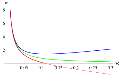
Figure 1: Diagrams for the three mass-temperature relations, ours (red), Hawking’s (green), and stringy GUP result (blue), with $\zeta=\sqrt{2}$, as an example. As a consequence of the lattice uncertainty principle the evaporation ends at a finite temperature with a zero rest-mass remnant.

 

Considering $m$ and $\Theta$ as functions of time, we can follow the evolution of a micro black hole from the curves in Fig. 1. For the stringy GUP, the blue line predicts a maximum temperature

$$\Theta_{{\rm max}}\ =\ \frac{1}{2\pi{\zeta}}\,,$$ (58a)

and a minimum rest mass

$$m_{{\rm min}}\ =\ {\zeta}\,.$$ (58b)

The end of the evaporation process is reached in a finite time, the final temperature is finite, and there is a remnant of a finite rest mass (cf. Refs. FS9506 ; ACSantiago ; Adler2 ; CavagliaD ; CDM03 ; nouicer ; Glimpses ; Casadio ).

From the standard Heisenberg uncertainty principle we find the green curve, representing the usual Hawking formula. Here the evaporation process ends, after a finite time, with a zero mass and a worrisome infinite temperature. In the literature, the undesired infinite final temperature predicted by Hawking’s formula has so far been cured only with the help of the stringy GUP, which brings the final temperature to a finite value. This result is, however, also questionable since it implies the existence of finite-mass remnants in the universe. Though by some authors such remnants are greeted as relevant candidates for dark matter chenDM , others point out that their existence would create further complications such as the entropy/information problem beken , detectability issue, or their (excessive) production in the early universe  Giddings:08 ; remnants .

In contrast to these results, our lattice GUP predicts the red curve. This yields a finite end temperature

$$\Theta_{{\rm max}}\ =\ \frac{1}{2\pi{\zeta}}\,,$$ (59)

with a zero-mass remnant. The mass-temperature formula (55) thus solves at once several problems by predicting the end of the evaporation process at a finite final temperature with zero-mass remnants.

Is should be stressed that since the photon GUP (43) and (49) holds only for states $\psi$ where $\langle\hat{p}^{2}\rangle_{\psi}\ll\hbar^{2}/\epsilon^{2}$, our reasonings are warranted only for

$$E_{\epsilon}\ \ll\ \hbar c/\epsilon\ \simeq\ \mathcal{E}_{p}/a\;\;\;\;\Rightarrow\;\;\;\;2\pi\zeta\ \ll\ \frac{1}{\Theta}\,.$$ (60)

This implies, in particular, that when $\Theta$ is close to $\Theta_{{\rm max}}$ our long-wavelength approximation cannot be trusted.

To understand the behavior of the system close to $\Theta_{{\rm max}}$ we must turn to the short-wavelength limit, Eqs. (33) and (46). In this regime the momenta lie close to the border of the Brillouin zone $\langle\hat{p}\rangle_{\psi}\simeq\langle\hat{P}_{\epsilon}\rangle_{\psi}\simeq\pi\hbar/(2\epsilon)$, and Eq. (40) implies

$$E_{\epsilon}\ \simeq\ \frac{\sqrt{2}}{\epsilon}\,\hbar c\,,$$ (61)

which for the Planckian lattice, where $\epsilon=a\,\ell_{p}$, gives $E_{\epsilon}\simeq\mathcal{E}_{p}/(\pi\,\zeta)$. Considering again the uncertainty in the photon position as $\delta X_{\epsilon}\simeq 2\pi\ell_{p}m$ (cf. Eq. (51)), GUP (46) then predicts

$$\delta X_{\epsilon}\ \propto\ m\ \simeq\ \frac{a}{2\pi^{2}}\left(1-\frac{a^{2}\ell_{p}^{2}}{2\hbar^{2}c^{2}}\frac{{\cal E}_{p}^{2}}{\pi^{2}\zeta^{2}}\,\right)\ =\ 0\,.$$ (62)

We can thus conclude that the mass of the micro black hole must go to zero. This is also consistent with our previous long-wavelength considerations. The micro black hole therefore evaporates completely, without leaving remnants.

VII Entropy and heat capacity

In this section we exhibit the modified thermodynamic entropy and heat capacity of a black hole implied by the new mass-temperature formula (55).

VII.1 Entropy

From the first law of black hole thermodynamics BCH we know that the differential of the thermodynamical entropy of a Schwarzschild black hole reads

$$dS\ =\ \frac{dE}{T_{H}}\,,$$ (63)

where $dE$ is the amount of energy swallowed by a black hole with Hawking temperature $T_{H}$. In Eq. (63) the increase in the internal energy is equal to the added heat because a black hole makes no mechanical work when its entropy/surface changes (expanding surface does not exert any pressure).

Rewriting Eq. (63) with the dimensionless variables $m$ and $\Theta$ we get

$$dS\ =\ \frac{k_{B}}{2}\frac{dm}{\Theta}\,.$$ (64)

Inserting here formula (55) we find

$$dS\ =\ \frac{k_{B}}{2}\frac{dm}{\Theta}\ =\ -\frac{k_{B}}{4}\left(\frac{1}{2\pi\Theta^{3}}+\frac{2\pi\zeta^{2}}{\Theta}\right)\,d\Theta\,.$$ (65)

By integrating $dS$ we obtain $S=S(\Theta)$. Just as formula (55), the relation (65) can be trusted only for $\Theta\ll\Theta_{\rm max}=1/2\pi\zeta$. Thus, when integrating (65), we should do this only up to a cutoff $\tilde{\Theta}_{\rm max}\ll\Theta_{\rm max}$. The additive constant in $S$ can be then be fixed by requiring that $S=0$ when $\Theta\to\tilde{\Theta}_{\rm max}$. This is equivalent to what is usually done when calculating the Hawking temperature for a Schwarzschild black hole. There one fixes the additive constant in the entropy integral to be zero for $m=0$, so that $S(m=0)=S(\Theta\rightarrow\infty)=0$ (the minimum mass attainable in the standard Hawking effect is $m=0$). Thus we obtain

$$S\ =\ \frac{k_{B}}{4}\int_{\Theta}^{\tilde{\Theta}_{\rm max}}\left(\frac{1}{2\pi\Theta^{\prime 3}}+\frac{2\pi\zeta^{2}}{\Theta^{\prime}}\right)\,d\Theta^{\prime}$$ (66)

where the sign was chosen in order to have a positive entropy.

The integral (66) yields

$$S(\Theta)\ =\ \frac{k_{B}}{16\,\pi}\left(\frac{1}{\Theta^{2}}-\frac{1}{\tilde{\Theta}_{\rm max}^{2}}+8\pi^{2}\zeta^{2}\log\frac{\tilde{\Theta}_{\rm max}}{\Theta}\right)\!.$$ (67)

The entropy is always positive, and $S\to 0$ for $\Theta\to\tilde{\Theta}_{\rm max}$.

VII.2 Heat Capacity

With entropy formulae (65) and (67) at hand we can now compute the heat capacity of a (micro) black hole in the world-crystal. This will give us important insights on the final stage of the evaporation process. Again, we shall obtain formulae valid only for $\Theta\ll\Theta_{\rm max}=1/(2\pi\zeta)$.

The heat capacity $C$ of a black hole is defined via the relation

$$dQ\ =\ dE\ =\ CdT\,.$$ (68)

The pressure exerted on the environment by the expanding black hole surface is zero. Hence we do not need to specify which $C$ is meant.

With the help of (63) and (68) we obtain

$$C\ =\ T\left(\frac{dS}{dT}\right)\ =\ \Theta\left(\frac{dS}{d\Theta}\right)\,,$$ (69)

which yields

$$C\ =\ -\frac{\pi k_{B}}{2}\left[\zeta^{2}+\frac{1}{(2\pi\Theta)^{2}}\right]\!.$$ (70)

From this clearly follows that $C$ is always negative.

Most condensed-matter systems have $C>0$. However, because of instabilities induced by gravity this is generally not the case in astrophysics thirring ; zeh , especially in black hole physics. A Schwarzschild black hole has $C<0$ which indicates that the black hole becomes hotter by radiating. The result (70) implies that this scenario holds also for micro black holes in the world-crystal.

In case of stringy GUP, we have to use Eq. (57) as the mass-temperature formula. The expression for the heat capacity then reads

$$C\ =\ \frac{\pi k_{B}}{2}\left[\zeta^{2}-\frac{1}{(2\pi\Theta)^{2}}\right]\!.$$ (71)

Since also here $0<\Theta<\Theta_{\rm max}=1/2\pi\zeta$, black holes have negative specific heat also according to the stringy GUP. However, stringy GUP displays a striking difference with respect to lattice GUP. In fact, since in principle we can trust Eq. (57) also when $\Theta\simeq\Theta_{\rm max}=1/2\pi\zeta$, then from (71) we have, in such limit, $C=0$. This means that for the stringy GUP the specific heat vanishes at the end point of the evaporation process in a finite time, so that the black hole at the end of its evolution cannot exchange energy with the surrounding space. In other words, the black hole stops to interact thermodynamically with the environment. The final stage of the Hawking evaporation, according to the stringy GUP scenario, contains a Planck-size remnant with a maximal temperature $\Theta=\Theta_{\rm max}$, but thermodynamically inert. The remnant behaves like an elementary particle — there are no internal degrees of freedom to excite in order to produce a heat absorption or emission.

To understand the heat exchange in the last live stage of the world-crystal black hole we cannot use the long-wavelength formula (70). Instead, we must turn to Eq. (46). Since in our scenario the micro black hole disappears at the critical temperature $\Theta_{\rm max}$, it is more appropriate to write the mass-temperature formula (46) in the form

$$m\ \simeq\ \theta(\Theta_{\rm max}-\Theta)\ \!\frac{\sqrt{2}}{\pi}\zeta\left(1\ -\ \frac{a^{2}}{8}\ \!\Theta^{2}\right)\!,$$ (72)

where $\theta(t)$ is the Heaviside step function. For the specific heat this implies

$$C\ \simeq\ -\theta(\Theta_{\rm max}-\Theta)\ \!\sqrt{2}\pi\ \!k_{B}\zeta^{3}\ \!\Theta\,.$$ (73)

So, in contrast to the stringy result, a world-crystal black hole exchanges heat with its environment by radiation until the last moment of its existence, and unlike the Schwarzschild black hole, the heat exchange with the environment increases in the final stage of its evaporation. In addition, because of the $\theta$-function in (73), the transition from the universe with the world-crystal black hole to the one without it is of first order.

VIII Further applications

So far we have studied the consequence of the GUP on the micro black holes. Let us briefly mention two further applications.

VIII.1 ’t Hooft’s proposal

The first application relates to ’t Hooft’s proposal which purports to justify that our quantum world is merely a low-energy limit of a deterministic system operating at a deeper, perhaps Planckian, level of dynamics tHoft1 ; tHoft2 . As a deterministic substrate ’t Hooft has proposed various cellular automata (CA) models.

In general, a CA is an array of cells forming a discrete lattice. All cells are typically equivalent and can take one of a finite number of possible discrete states. Like space, time is discrete as well. At each time step every cell updates its state according to a transition rule which takes into account the previous states of cells in the neighborhood, including its own state. In this sense the evolution is deterministic.

One of the simplest CA considered by ’t Hooft is the $1$-dimensional periodic CA with $4$-state cells, and with the nearest neighbor (N-N) transition rule, see Fig. 2.

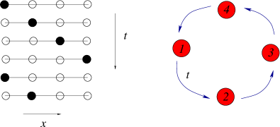
Figure 2: CA with discrete time evolution described by Eq.  (74) and with the periodicity condition $\sigma_{i}=\sigma_{i+4}$. The right-hand shows an equivalent graphical representation.

 

This “clock like” CA can be generally described with $2N+1$ cells $\sigma_{i}~{}(i=-N,\ldots,N)$ each with two possible states $\{0,1\}$ (cell is, e.g., white or black). The discrete time evolution with the elementary time step $\delta t$ is described by the N-N transition rule

$$\mbox{}(\sigma_{i-1},\sigma_{i},\sigma_{i+1})\ \rightarrow\ \sigma^{\prime}_{i}\ =\ \sigma_{i}(t+\delta t):$$

$$\mbox{}(0,0,0)\rightarrow 0,\;\;(0,0,1)\rightarrow 0,\;\;(0,1,0)\rightarrow 0,$$

$$\mbox{}(1,0,0)\rightarrow 1,\;\;(1,1,0)\rightarrow 0,\;\;(0,1,1)\rightarrow 0,$$

$$\mbox{}(1,0,1)\rightarrow 0,\;\;(1,1,1)\rightarrow 0\,,$$ (74)

with the Born-von Karman periodicity condition $\sigma_{i}=\sigma_{i+2N+1}$.

The cells can be algebraically represented by orthonormal vectors

$$\sigma_{-N}=\left(\begin{array}[]{c}0\\ 0\\ \vdots\\ 1\end{array}\right)\!;\;\sigma_{-N+1}=\left(\begin{array}[]{c}1\\ 0\\ \vdots\\ 0\end{array}\right)\!;\;\ldots\;\sigma_{N}=\left(\begin{array}[]{c}0\\ \vdots\\ 1\\ 0\end{array}\right)\!,$$

$\sigma_{-N}=\sigma_{N+1}$. On the basis spanned by $\sigma_{i}$ the elementary-time step evolution operator is:

$$\mbox{}\hat{U}(\delta t=\tau)=e^{-i\hat{H}\delta t}=e^{-i\frac{\pi}{2N+1}}\!\left(\begin{array}[]{ccccc}0&&&&1\\ 1&0&&&\\ &&\ddots&\ddots&\\ &&&1&0\end{array}\right)\!,$$ (80)

which, among others, defines the Hamiltonian $\hat{H}$. The pre-factor $e^{-i\frac{\pi}{2N+1}}$ is known as ’t Hooft’s phase convention. Because $\hat{U}^{{2N+1}}=-\hat{\openone}$ one can diagonalize $\hat{U}$ as

$$\hat{U}_{\rm{diag}}\ =\ e^{-i\frac{\pi}{2N+1}}\ \mbox{diag}\!\left(e^{-i\frac{2\pi N}{2N+1}},\ldots,1,\ldots,e^{i\frac{2\pi N}{2N+1}}\right)\,.$$

If we denote the eigenstates of $\hat{H}$ as $|n\rangle$, we find that

$$|n\rangle\ =\ \frac{1}{\sqrt{2N+1}}\sum_{\ell=-N}^{N}\exp\left[-{i\frac{2\pi n}{2N+1}\ \!\ell}\right]\sigma_{\ell}\,,$$ (81)

with $n=-N,\ldots,N$ and the ensuing “energy” spectrum reads

$$\hat{H}|n\rangle\ =\ \omega_{N}\,\left(n+\mbox{$\frac{1}{2}$}\right)|n\rangle,\;\;\;\;\omega_{N}\equiv\frac{2\pi}{(2N+1)\delta t}\,.$$ (82)

The energy values $E_{n}$ resemble the spectrum of the harmonic oscillator, except that the $n$’s are bounded and can attain negative values. We shall be coming back to this issue shortly.

Position and momentum can be represented by operators with the matrix representations

$$\hat{X}_{\epsilon} = \left(\begin{array}[]{ccccc}(-N+1)\epsilon&0&0&\cdots&0\\ 0&(-N+2)\epsilon&0&&0\\ \vdots&&\ddots&&\vdots\\ 0&\cdots&&N\epsilon&0\\ 0&\cdots&&0&-N\epsilon\end{array}\right)\!,$$ (88)

$$\hat{P}_{\epsilon} = \ \frac{1}{2i\epsilon}\!\left(\begin{array}[]{cccccc}0&1&0&0&\cdots&-1\\ -1&0&1&0&\cdots&0\\ 0&-1&0&1&\cdots&0\\ \vdots&&&\ddots&&\vdots\\ 0&0&\cdots&&0&1\\ 1&0&\cdots&&-1&0\end{array}\right)\!,$$ (95)

where $\epsilon=2\pi/(2N+1)$. With these we obtain the commutator

$$[\hat{X}_{\epsilon},\hat{P}_{\epsilon}]\ =\ \frac{i}{2}\left(\begin{array}[]{cccccc}0&1&0&0&\cdots&1\\ 1&0&1&0&\cdots&0\\ 0&1&0&1&\cdots&0\\ \vdots&&&\ddots&&\vdots\\ 0&0&\cdots&&0&1\\ 1&0&\cdots&&1&0\end{array}\right)\!.$$ (102)

In deriving (102) we have used the the periodicity condition $\sigma_{-1}=\sigma_{2N}$. By comparing this with the evolution operator (80) we have

$$[\hat{X}_{\epsilon},\hat{P}_{\epsilon}]\ =\ i\cos[(\hat{H}-\omega_{N}/2)\delta t]\,,$$ (103)

which for small $\delta t$ gives

$$[\hat{X}_{\epsilon},\hat{P}_{\epsilon}]\ \simeq\ i\left[1-\frac{\delta t^{2}}{2}(\hat{H}-\omega_{N}/2)^{2}\right]\!.$$ (104)

In addition, we deduce from (80) and (95) that

$$\sin[(\hat{H}-\omega_{N}/2)\delta t]\ =\ \epsilon\hat{P}_{\epsilon}\,,$$ (105)

which is compatible with the result (20). From (105) follows that $\hat{H}$ depends only on $\hat{P}_{\epsilon}$ but not on $\hat{X}_{\epsilon}$. So $\hat{P}_{\epsilon}$ and $\hat{H}$ are simultaneously diagonalizable. By defining the operators $\hat{K}_{\pm}$ as

$$\hat{K}_{+}\ = \ e^{-i\hat{X}_{\epsilon}}\hat{P}_{\epsilon},\;\;\;\;\;\hat{K}_{-}\ =\ \hat{P}_{\epsilon}\ \!e^{i\hat{X}_{\epsilon}}\,,$$ (106)

($\hat{K}_{-}=\hat{K}_{+}^{{\dagger}}$), so that

$$\mbox{}\hat{K}_{+}|n\rangle = \frac{2N+1}{2\pi}\sin\left[\frac{2\pi}{2N+1}\ \!n\right]\ \!|n+1\rangle\,,$$

$$\mbox{}\hat{K}_{-}|n\rangle = \frac{2N+1}{2\pi}\sin\left[\frac{2\pi}{2N+1}(n-1)\right]\ \!|n-1\rangle\,,$$ (107)

one can persuade itself that $\hat{H}$ and $\hat{K}_{\pm}$ close the deformed algebra which in the large $N$ limit (i.e., in the small $\epsilon$ or $\delta t$ limit) reduces to

$$[\hat{H},\hat{K}_{\pm}]\ =\ \pm\ \!\omega\hat{K}_{\pm},\;\;\;\;\;[\hat{K}_{+},\hat{K}_{-}]\ =\ -\frac{2\hat{H}}{\,\omega}\,,$$ (108)

with $\omega=\omega_{\infty}$.

Note that for large $N$ one can identify (82), (107), and (108) with the representation of $SU(1,1)$ known as the discrete series $D^{+}_{1/2}\oplus D^{-}_{1/2}$ (cf. Ref. JBV ). Generally, the Lie algebra $D^{+}_{k}\oplus D^{-}_{k}$ is defined through the relations:

$$\hat{L}_{3}|k,m\rangle\ =\ (m+k)|k,m\rangle\,,$$

$$\hat{L}_{+}|k,m\rangle\ =\ \sqrt{(m+2k)(m+1)}\ |k,m+1\rangle\,,$$

$$\hat{L}_{-}|k,m\rangle\ =\ \sqrt{(n+2k-1)m}\ |k,m-1\rangle\,,$$

$$[\hat{L}_{3},\hat{L}_{\pm}]\ =\ \pm\hat{L}_{\pm},\;\;\;\;\;[\hat{L}_{+},\hat{L}_{-}]\ =\ -2\hat{L}_{3}\,.$$ (109)

Here $m+k=\pm k,\pm(k+1),\pm(k+2),\ldots$ and $k=\frac{1}{2},1,\frac{3}{2},2,\ldots$ is the so-called Bargmann index which labels the representations. From this we have that $D^{+}_{1/2}\oplus D^{-}_{1/2}$ corresponds to

$$\hat{L}_{3}|\raisebox{0.40903pt}{\scriptsize${\frac{1}{2}}$},m\rangle\ =\ (m+1/2)|\raisebox{0.40903pt}{\scriptsize${\frac{1}{2}}$},m\rangle\,,$$

$$\hat{L}_{+}|\raisebox{0.40903pt}{\scriptsize${\frac{1}{2}}$},m\rangle\ =\ (m+1)|\raisebox{0.40903pt}{\scriptsize${\frac{1}{2}}$},m+1\rangle\,,$$

$$\hat{L}_{-}|\raisebox{0.40903pt}{\scriptsize${\frac{1}{2}}$},m\rangle\ =\ m|\raisebox{0.40903pt}{\scriptsize${\frac{1}{2}}$},m-1\rangle\,,$$ (110)

Identification with the large-$N$ limit of (82) and (107) is established when we identify $\hat{H}$ in (110) with $\omega\hat{L}_{3}$, $\hat{K}_{\pm}$ with $\hat{L}_{\pm}$, and set $m=n$.

At this stage one can invoke ’t Hooft’s loss of information condition tHoft1 ; tHoft2 , and project out the negative part of the spectra. A plausible rationale for this step can be found, e.g., in irreversibility of computational process due to a finite storage capacity JBV2 .

After the negative energy spectrum is removed (erased), we obtain only the positive discrete series $D_{{1}/{2}}^{+}$ (i.e., representation where $m=0,1,2,\ldots$), and the Hamiltonian morphs into a non-negative spectrum Hamiltonian $H^{+}$.

The usual $W(1)$-algebra of the quantum harmonic oscillator emerges after we introduce the following mapping in the universal enveloping algebra of $SU(1,1)$:

$$\mbox{}\hat{a}\ =\ \frac{1}{\sqrt{\hat{L}_{3}+1/2}}\,\hat{L}_{-},\;\;\;\;\hat{a}^{\dagger}\ =\ \hat{L}_{+}\,\frac{1}{\sqrt{\hat{L}_{3}+1/2}}\,.$$ (111)

The latter gives a one-to-one (non-linear) mapping between the deterministic cellular automaton system (with information loss) and the quantum harmonic oscillator. The reader will recognize the mapping Eq. (111) as the non-compact analog gerry of the well-known Holstein-Primakoff representation for $SU(2)$ spin systems holstein .

Our operators $\hat{X}_{\epsilon}$, $\hat{P}_{\epsilon}$ and $\hat{I}_{\epsilon}$ may be viewed as the same cellular automaton $E(2)$ algebra as discussed in Section III. Thus we can conclude that in the Planckian scale the system must behave deterministically — which is one of the defining property of cellular automata. It is only at low energies when the loss of information leads to the emergent degrees of freedom resulting in the usual quantum mechanical description

VIII.2 Double special relativity

The second application relates to the idea of double (or doubly or deformed) special relativity (DSR) (see, e.g., Refs. DSR ; MS ). The general idea is that if the Planck length is a truly universal quantity, then it should look the same to any inertial observer. This demands a modification (deformation) of the Lorenz transformations, to accommodate an invariant length scale. In Ref. MS the nonlinearity of the deformed Lorenz transformations lead the authors to novel commutators between spacetime coordinates and momenta, depending on the energy

$$\left[{\hat{x}}^{i},{\hat{p}}_{j}\right]={\rm i}\hbar\left(1-\frac{E}{{\cal E}_{p}}\right)\delta^{i}_{j}\,,$$ (112)

where $E$ is the energy scale of the particle to which the deformed Lorenz boost is to be applied, while ${\cal E}_{p}$ is the Planck energy. This suggests that they have an energy-dependent Planck “constant” $\hbar(E)=\hbar(1-E/{\cal E}_{p})$. Their model also implies that $\hbar(E)\to 0$ for $E\to{\cal E}_{p}$. For energies much below that Planck regime, the usual Heisenberg commutators are recovered, but when $E\simeq{\cal E}_{p}$ one has $\hbar({\cal E}_{p})\simeq 0$. So the Planck energy is not only an invariant in this model, but the world looks also apparently classical at the Planck scale, similarly as in ’t Hooft’s proposal.

The connections of the DSR model with our proposal are at this point self evident. Our GUP (22), (24) implies that, at the boundary of the Brillouin zone, when $\langle\hat{p}\rangle_{\psi}\to\hbar\pi/2\epsilon$, i.e. for Planck energies $E_{\epsilon}\simeq(2\sqrt{2}/a){\cal E}_{p}$, the fundamental commutator vanishes

$$[\hat{X}_{\epsilon},\hat{P}_{\epsilon}]\simeq 0\,,$$ (113)

and since

$$\Delta X_{\epsilon}\Delta P_{\epsilon}\ \gtrsim\ 0\,,$$ (114)

lattice quantum mechanics at short wavelengths allows for classical behavior, that is uncertainties of two complementary observables can be simultaneously zero.

However, if we express the fundamental commutator (22) of our model in terms of energy, using the exact relation (40), we find (for $\epsilon=a\ell_{p}$)

$$\left[\hat{X}_{\epsilon},\hat{P}_{\epsilon}\right]f(x)\ = \ i\hbar\left(1-\frac{a^{2}}{8}\frac{\hat{E}^{2}}{{\cal E}^{2}_{p}}\right)f(x)\,.$$ (115)

This means that the deforming term in our model is quadratic in the energy, instead of the linear dependence in the energy of the DSR model (112).

IX Discussion and Summary

It should be noted that the present lattice generalization of the uncertainty principle is not an approximate description, but it is an exact formula necessarily implied by our model of lattice space time. The great majority of the GUP research has always borrowed the deformed commutator $[\hat{x},\hat{p}]=i\hbar(1+\kappa\hat{p}^{2})$ either from string theory, or from heuristic arguments about black holes veneziano ; mascad . To be precise, even in string theory veneziano the formula expressing the GUP is not derived from the basic features of the model, but instead it is deduced from high-energy gedanken experiments of string scatterings. In contrast to this we have derived all results from a simple lattice model of spacetime, and from the analytic structure of the basic commutator (22).

We have calculated the uncertainties on a crystal-like universe whose lattice spacing is of the order of Planck length — the so-called world crystal. When the energies lie near the border of the Brillouin zone, i.e., for Planckian energies, the uncertainty relations for position and momenta do not pose any lower bound on the associated uncertainties. Hence the world crystal universe can become“deterministic” at Planckian energies. In this high-energy regime, our lattice uncertainty relations resemble the double special relativity result of Magueijo and Smolin.

The scenario in which the universe at Planckian energies is deterministic rather than being dominated by quantum fluctuations is a starting point in ’t Hooft’s “deterministic” quantum mechanics.

With the generalized uncertainty relation at hand we have been able to derive a new mass-temperature relation for Schwarzschild micro black holes. In contrast to standard results based on Heisenberg or stringy uncertainty relations, our mass-temperature formula predicts both finite Hawking’s temperature and a zero rest-mass remnant at the end of the evaporation process. Especially the absence of remnants is a welcome bonus which allows to avoid such conceptual difficulties as entropy/information problem or why we do not experimentally observe the remnants that must have been prodigiously produced in the early universe.

Apart from the mass-temperature relation we have also computed two relevant thermodynamic characteristics, namely entropy and heat capacity. Particularly the heat capacity provided an important insight into the last life stage of the world-crystal micro black holes. In contrast to the stringy result, our result indicates that world-crystal micro black hole exchanges heat with its environment (radiate) till the last moment of its existence, and unlike the Schwarzschild micro black hole, the heat exchange with the environment increases in the final stage of the evaporation. In addition, the transition from the universe with the world-crystal micro black hole to the one without is of the first order.

Since the world crystal physics allows for deterministic description of the physics at Planckian energies, we have included in this paper a discussion of ’t Hooft’s periodic automaton model which gives at low energy scales rise to a genuine quantum harmonic oscillator. In addition, such an automaton has a close connection with our world crystal paradigm. Here we have re-derived ’t Hooft’s result in a new way. In contrast to ’t Hooft derivation tHoft2 we have matched the algebra of the automaton variables with the $SU(1,1)$ algebra, and in contrast to Ref. JBV we have worked with a different set of dynamical variables. In the contraction limit (i.e., in the limit of many lattice spacings — low energy limit) we have recovered the canonical $W(1)$-algebra and were able to identify the “emergent” harmonic oscillator variables.

There are several aspects of the double special relativity that are worth noting in the connection with our generalized uncertainty relation. Essentially, we have seen that the fundamental commutator in DSR as well as in our lattice GUP goes to zero at Planck energy. For both models, the world should therefore be manifestly ”classical” in the Planck regime, a feature very different from the common believe. This is a striking prediction supported by both models, although the lines of thought followed in the two research paths are completely different and independent. Moreover, this aspect presents also a strong resemblance with the results obtained in the research line of “deterministic” quantum mechanics.

X Acknowledgements

One of us (P.J.) is grateful to G. Vitiello for instigating discussions. This work was partially supported by the Ministry of Education of the Czech Republic (research plan MSM 6840770039), and by the Deutsche Forschungsgemeinschaft under grant Kl256/47. F.S. acknowledges financial support by the National Taiwan University under the contract NSC 98-2811-M-002-086, and thanks ITP Freie Universität Berlin for warm hospitality.

Appendix: Landauer principle

Here we wish to provide an alternative derivation of the mass-temperature formula (55) based on Landauer’s principle. To this end we consider an ensemble of unpolarized photons that are going to deliver to a micro black hole one single bit of information per particle. In order to be sure that each photon delivers only one bit of information — namely the information that it is there, somewhere inside in the black hole, its position uncertainty must be “maximal”, i.e., it should not be smaller than Schwarzschild’s radius $R_{S}$ as otherwise the photon would deliver to black hole also extra bits of information concerning its entry point (or better sector) on the horizon. At the same time its wavelength should not be bigger than $R_{S}$, as otherwise the photon would bounced off the black hole without getting trapped. In this view, the position uncertainty of a photon in the ensemble must be of order of Schwarzschild’s radius $R_{S}$ i.e., $\Delta X_{\epsilon}\simeq\mu R_{S}$. Factor $\mu$ is Bekenstein’s deficit coefficient which ensures a correct Hawking’s formula in a continuum limit.

An extra bit of information added to the micro black hole will increase its energy at least by amount $\Delta E_{\epsilon}$ so that (cf. (43))

$$\Delta X_{\epsilon}\Delta E_{\epsilon}\ \simeq\ \frac{\hbar c}{2}\left[1-\frac{\epsilon^{2}}{2\hbar^{2}c^{2}}\ \!(\Delta E_{\epsilon})^{2}\right].$$ (116)

In the following we denote $\Delta E_{\epsilon}$ simply as $E_{\epsilon}$ to stress that $\Delta E_{\epsilon}$ an energy increas due to one photon. With the explicit form for Planck’s energy

$$\mathcal{E}_{p}\ =\ \frac{\hbar c}{2\ell_{p}}\ \approx\ 0.61\cdot 10^{19}\ \!\mbox{GeV}\,,$$ (117)

the relation (116) can be cast to

$$\Delta X_{\epsilon}\ \simeq\ \frac{\hbar c}{2E_{\epsilon}}-\frac{a^{2}\ell_{p}E_{\epsilon}}{8\mathcal{E}_{p}}\,.$$ (118)

If we use further the fact that, $R_{S}=\ell_{p}\,m$, where $m$ is the relative mass of the black hole in Planck units, i.e., $m=M/M_{p}$ ($M_{p}=\mathcal{E}_{p}/c^{2}$), we can rewrite (118) as

$$2m\mu\ \simeq\ \frac{\mathcal{E}_{p}}{E_{\epsilon}}-\frac{a^{2}E_{\epsilon}}{8\mathcal{E}_{p}}\,.$$ (119)

According to the Landauer principle landauer:61 , when a single bit of information is erased (like in the black hole) the amount of energy dissipated into environment is at least $k_{B}T\ln 2$, where $k_{B}$ is Boltzmann’s constant and $T$ is the temperature of the erasing environment (in our case the micro black hole). Since the liberated energy per bit of lost information can not be grater the energy $E_{\epsilon}$ of the carrier photon we have that

$$E_{\epsilon}\ \simeq\ k_{B}T\,.$$ (120)

Relation (120) basically expresses equipartition law for an unpolarized photon in the outgoing Hawking radiation. Defining the Planck temperature $T_{p}=2\mathcal{E}_{p}/k_{B}\approx 3\cdot 10^{32}$ K, and measuring the temperature in terms of Planck units as a relative temperature $\Theta=T/T_{p}$, we can rewrite Eq. (119) in the form

$$2m\ =\ \frac{1}{2\pi\Theta}-2\pi\zeta^{2}\Theta\,.$$ (121)

where we identify $\zeta=a/(2\sqrt{2}\pi)$ and set $\mu=\pi$, in order to agree with (55) and with Hawking’s formula (56) in the continuum limit.

References

- (1) E. Witten, Physics Today 49 (1996) 24.
- (2) L.J. Garay, Phys. Rev. Lett. 80 (1998) 2508.
- (3) C. Rovelli, Quantum Gravity, (Cambridge University Press, Cambridge, 2004).
- (4) R. Gambini and J. Pullin, J. Phys. Rev. D 59 (1999) 124021.
- (5) J. Alfaro, H.A. Morales-Tecotl and L.F. Urrutia Phys. Rev. Lett. 84 (2000) 2318.
- (6) G. Amelino-Camelia and S. Majid Int. J. Mod. Phys. A 15 (2000) 4301.
- (7) A. Matusis, L. Susskind and N. Toumbas J. High Energy Phys. JHEP0012 (2000) 002.
- (8) G. Amelino-Camelia Phys. Lett. B 510 (2001) 255.
- (9) N.R. Douglas and N.A. Nekrasov Rev. Mod. Phys. 73 (2001) 977.
- (10) T. Jacobson and A.C. Wall, [arXiv:0804.2720].
- (11) T. Toffoli, IEEE Computer Society Press (1993) 5; Bull.It.Assoc.Artificial Intelligence 14 (2001) 32
- (12) S. Wolfram, Rev. Mod. Phys. 55 (1983) 601.
- (13) S. Wolfram., A New Kind of Science, (Wolfram Media, Champaign, IL, 2002).
- (14) ’t Hooft G., J. Stat. Phys. 53 (1988).
- (15) ’t Hooft G., in 37th Int. School of Subnuclear Phys., Erice, Ed. A. Zichichi, (World Scientific, London, 1999).
-
(16)
See the homepage:
http://www.sciops.esa.int/
index.php?project=PLANCK - (17) See the homepage: http://icecube.wisc.edu/
- (18) M. Creutz, Quarks, gluons and lattices, (Cambridge Univ. Press, Cambridge, 1983).
- (19) H. Kleinert, Gauge Fields in Condensed Matter, Vol. I Superflow and vortex lines. Disorder fields, phase transitions, (World Scientific, Singapore, 1989) (http://www.physik.fu-berlin.de/~kleinert/b1)
- (20) H. Kleinert, Gauge Fields in Condensed Matter, Vol. II Stresses and Defects, (World Scientific, Singapore, 1989) (http://www.physik.fu-berlin.de/~kleinert/b2)
- (21) R. Friedberg and T.D. Lee, Nucl. Phys. B 225 (1983) 1.
- (22) R. Friedberg and T.D. Lee, Nucl. Phys. B 245 (1983) 343.
- (23) H. Kleinert, Multivalued Fields in Condensed Matter, Electromagnetism, and Gravitation, (World Scientific, Singapore, 2008).
- (24) The appeal of such a description of geometry has recently been recognized also by G. ’t Hooft in various summer school lectures, for instance in Erice 2008 http://www.phys.uu.nl/~thooft/lectures/Erice_08.pdf and in Pescara 2008 http://www.icra.it/ICRA_Networkshops/INW25_Stueckelberg3/Welcome.html.
- (25) H. Kleinert, Ann. d. Physik 44 (1987) 117.
-
(26)
N. Arkani-Hamed, S. Dimopoulos, and G. Dvali,
Phys. Lett. B 429(1998) 263;
[hep-ph/9803315].
I. Antoniadis, N. Arkani-Hamed, S. Dimopoulos, and G. Dvali, Phys. Lett. B 436 (1998) 257; [hep-ph/9804398]. - (27) S.B. Giddings and M.L. Mangano, Phys. Rev. D 78 (2008) 035009.
- (28) A. Barrau, J. Grain and S.O. Alexeyev, Phys. Lett. B 584 (2004) 114.
- (29) A. Connes, Publ. I.H.E.S 62 (1986) 257.
- (30) A. Dimakis and F. Müller–Hoissen, Phys. Let. B 295 (1992) 242.
- (31) A. Dimakis, F. Müller–Hoissen and T. Striker, J. Phys. A 26 (1993) 1927.
- (32) E. Celeghini, S.De Martino, S.De Siena, M. Rasetti and G. Vitiello, Ann. Phys. 241 (1995) 50.
- (33) E. Schrödinger, Sitzungsber. Preuss. Acad. Wiss. 24 (1930) 296.
- (34) H.P. Robertson, Phys. Rev. 34 (1929) 163.
- (35) A. Messiah, Quantum Mechanics 2 Volumes, (Dover Publications Inc., New York, 2003)
- (36) J. Magueijo and L. Smolin, Phys. Rev. D 67 (2003) 044017.
- (37) G. ‘t Hooft, Class. Quant. Grav. 16 (1999) 3263; [gr-qc/9903084]; [hep-th/0105105].
- (38) G. ‘t Hooft, Int. J. Theor. Phys. 42 (2003) 355; [hep-th/0104080]; [hep-th/0104219].
- (39) H.-T. Elze, Phys. Lett. A 310 (2003) 110; J. Phys. Conf. Ser. 174 (2009) 012009.
- (40) T.S. Biro, S.G. Matinyan and B. Muller, Found. Phys. Lett. 14(2001) 471.
- (41) R. Banerjee, Mod. Phys. Lett. A 17 (2002) 631.
- (42) J.J. Halliwell, Phys. Rev. D 63 (2001) 085013.
- (43) M. Blasone, P. Jizba, G. Vitiello, Phys. Lett. A 287 (2001) 205.
- (44) F. Scardigli, Nuovo Cim. B 110 (1995) 1029.
- (45) R.J. Adler, P. Chen and D.I. Santiago, Gen. Rel. Grav. 33 (2001) 2101.
- (46) P. Chen and R.J. Adler, Nucl. Phys. Proc. Suppl. 124 (2003) 103.
- (47) M. Cavaglia and S. Das, Class. Quant. Grav. 21 (2004) 4511.
- (48) M. Cavaglia, S. Das and R. Maartens, Class. Quant. Grav. 20 (2003) L205.
- (49) L. Susskind, J. Lindesay, An Introduction to Black Holes, Information, and the String Theory Revolution (World Scientific, Singapore, 2005). See chapter 10.
- (50) K. Nouicer, Class. Quant. Grav. 24, (2007) 5917.
- (51) F. Scardigli, Glimpses on the micro black hole planck phase, [arXiv:0809.1832].
- (52) R. Casadio, P. Nicolini, JHEP 0811, (2008) 072.
- (53) H. Kleinert, Phys. Lett. A 91 (1982) 295.
- (54) W. Heisenberg, Zeitschrift für Physik, 43 (1927) 172.
- (55) G. Veneziano, Europhys Lett. 2 (1986) 199; D. Amati, M. Ciafaloni, G. Veneziano, Phys. Lett. B 197 (1987) 81; D.J. Gross, P.F. Mende, Phys. Lett. B 197, (1987) 129; D. Amati, M. Ciafaloni and G. Veneziano, Phys. Lett. B 216 (1989) 41; G. Veneziano, Quantum Gravity near the Planck scale, Talk at PASCOS 90, Boston PASCOS 486 (1990); K. Konishi, G. Paffuti, P. Provero, Phys. Lett. B 234, (1990) 276; R. Guida, K. Konishi and P. Provero, Mod. Phys. Lett. A 6 (1991) 1487.
- (56) M. Maggiore, Phys. Lett. B 304 (1993) 65; F. Scardigli, Phys. Lett. B 452 (1999) 39; R.J. Adler and D.I. Santiago, Mod. Phys. Lett. A 14 (1999) 1371.
- (57) P. Chen, Mod. Phys. Lett. A 19 (2004) 1047; New Astron. Rev. 49 (2005) 233.
- (58) J.D. Bekenstein, Phys. Rev. D 49 (1994) 1912; S.B. Giddings, The black hole information paradox hep-th/9508151.
- (59) B.J. Carr and S.W. Hawking, Mon. Not. Roy. Astron. Soc. 168 (1974) 399; K. Nozari, Astroparticle Physics 27 (2007) 169; A. Barrau, C. Feron and J. Grain, Astrophys.J. 630 (2005) 1015.
- (60) J.M. Bardeen, B. Carter, S.W. Hawking, Commun. Math. Phys. 31 (1973) 161.
- (61) W. Thirring, Z. Physik 239 (1970) 339.
- (62) H.D. Zeh, The Physical Basis of the Direction of Time (Springer, Berlin, 1992).
- (63) M. Blasone, P. Jizba and G. Vitiello, J. Phys. Soc. Jap. Suppl. 72 (2003) 50; M. Blasone and P. Jizba, Can. J. Phys. 80 (2002) 645; M. Blasone, E. Celeghini, P. Jizba and G. Vitiello, Phys. Lett. A 310 (2003) 393.
- (64) M. Blasone and P. Jizba, J. Phys.: Conf. Ser. 67 (2007) 012046.
- (65) C. C. Gerry, J. Phys. A 16 (1983) L1.
- (66) T. Holstein and H. Primakoff, Phys. Rev. 58 (1940) 1098; M. N. Shah, H. Umezawa and G. Vitiello, Phys. Rev. B 10 (1974) 4724.
- (67) G. Amelino-Camelia, Int. J. Mod. Phys. D 11 (2002) 35; J. Magueijo and L. Smolin, Phys. Rev. Lett. 88 (2002) 190403; G. Amelino-Camelia, Nature 418 (2002) 34.
- (68) see, e.g., H.S. Leff and A.F. Rex, Maxwell’s Demon: Entropy, Information, Computing (Princeton University Press, Princeton, 1990).