Solution of an associating lattice gas model with density anomaly on a Husimi lattice

Abstract

We study a model of a lattice gas with orientational degrees of freedom which resemble the formation of hydrogen bonds between the molecules. In this model, which is the simplified version of the Henriques-Barbosa model, no distinction is made between donors and acceptors in the bonding arms. We solve the model in the grand-canonical ensemble on a Husimi lattice built with hexagonal plaquettes with a central site. The ground-state of the model, which was originally defined on the triangular lattice, is exactly reproduced by the solution on this Husimi lattice. In the phase diagram, one gas and two liquid (high density-HDL and low density-LDL) phases are present. All phase transitions (GAS-LDL, GAS-HDL, and LDL-HDL) are discontinuous, and the three phases coexist at a triple point. A line of temperatures of maximum density (TMD) in the isobars is found in the metastable GAS phase, as well as another line of temperatures of minimum density (TmD) appears in the LDL phase, part of it in the stable region and another in the metastable region of this phase. These findings are at variance with simulational results for the same model on the triangular lattice, which suggested a phase diagram with two critical points. However, our results show very good quantitative agreement with the simulations, both for the coexistence loci and the densities of particles and of hydrogen bonds. We discuss the comparison of the simulations with our results.

I Introduction

The introduction of orientational degrees of freedom in lattice gas models may result in rich phase diagrams. As an example, we may mention the study of lattice gas models with direction dependent interactions which were found to exhibit closed loop coexistence curves aw79 , such as the ones found in solutions of glycerol with guaiacol m23 , $m$-toluidine p24 , and ethylbenzylamine m23 , which exhibit a nearly symmetric coexistence loop with both an upper and a lower critical solution temperature. It was suggested by Hirschfelder, Stevenson, and Eyring hse37 , that the low-temperature critical point might be due to a highly directional short-range interaction, such as a hydrogen bond: while at low temperature the ordering of these interactions lowers the energy of solution, with rising temperature this ordering is decreased and phase separation occurs. These suggestion was followed in the model proposed by Barker and Fock some time later bf53 , and the solution of this model in the quasi-chemical approximation actually displays a closed coexistence loop. A simplified version of the model defined on a conveniently decorated simple cubic lattice, may be mapped on the three-dimensional Ising model and thus much precise information is known about its thermodynamic behavior w75 . When the directionality of the part of the interactions in the model due to the hydrogen bonds is increased, the results are closer to the experimental data for the mixtures cited above, although the correspondence to the Ising model is lost aw79 .

In water, the ordering of hydrogen bonds is supposed to be important in determining the unusual thermodynamic and dynamic behavior, including the possible existence of an experimentally unaccessible liquid-liquid phase transition d03 . Liquid-liquid phase transitions were originally found by Monte Carlo simulations of realistic liquid water models with atomic details p92 ; h97 , but they were already observed experimentally in systems such as phosphorus k00 , triphenyl phosphite k04 and $n$-butanol k05 ; t04 . Tetrahedral liquids, such as silica and water, also present thermodynamic and dynamic anomalies which can possibly be related to the second critical point (SCP) associated with these transitions e01 ; s06 ; s02 ; x05 ; k07 . Among these anomalous features, we note the increase of density with temperature that happens in liquid water at temperatures below $4^{o}C$ and the apparent divergent behavior of thermodynamic response functions with decreasing temperatures towards the deep super-cooled liquid, at atmospheric pressures d03 .

Several lattice models with orientational interactions, usually called network-forming fluids or associating lattice gases, have been proposed in two- b70 ; b04 ; h05 ; s93 ; gs02 and three-dimensions b72 ; b97 ; r96 ; p04 ; g07 to investigate the thermodynamic anomalies presented by water and tetrahedral liquids. Some of them were also found to present dynamic anomalies similar to the ones in liquid water s07 ; gs07 ; kf08 . In these models, the distinction between hydrogen bonds and van der Waals interactions is essential: these two main ingredients contribute to the appearance of a competition between distinct molecular states presenting high density (lowly bonded) and low density (highly bonded) structures. Nevertheless, in many models, more specific molecular interactions, and structures, are used to bias the system towards a low density liquid (LDL), at low pressures, or a high density liquid (HDL), at high pressures. As an example, some models use many-body interactions to unfavor molecular packing in the neighborhood of a hydrogen bond b04 ; b72 ; r96 ; p04 . Others actually energetically favor the LDL states through a repulsive van der Waals interaction b97 ; h05 ; g07 . Some implement fluctuating bonding structures gs02 , additional unbounded molecular states (to stabilize a disordered anomalous liquid) b04 ; r96 ; p04 and some even use ad hoc variations of volume with bond formation gs02 .

Considering the increasing complexity found in models for water in the literature hb , simple three- and two-dimensional models of liquid water, including only van der Waals and hydrogen bond interactions, have been investigated with the aim of finding the minimal requirements for water-like anomalous behavior h05 ; g07 ; s07 ; gs07 ; hg05 ; b07 ; b08 . One of these models, the GBHB model proposed by Girardi et al.g07 , is a three-dimensional fluid, defined on a body centered cubic lattice, with first-neighbor van der Waals and hydrogen-bond like interactions. It presents a phase diagram with two distinct liquid phases (high-density and low-density liquid - HDL and LDL) besides a GAS phase. Two coexistence lines (GAS-LDL and LDL-HDL) ending at critical points were originally found with Monte Carlo simulations by Girardi et al.g07 . Also, the isobars present temperatures of maximum density (TMD) on a line in the pressure-temperature plane, resembling qualitatively the scenario emerging from the simulations by Poole et al p92 . Nevertheless, a qualitatively different phase diagram was found for the same model in a recent work by Buzzano and collaborators bs08 , in which the phase diagrams of a three-dimensional model of network forming fluid g07 were investigated using the cluster variational method p03 . With this approach they were able to show that the topology of the phase diagram of the model was much more complex than originally found with Monte Carlo simulations but, at the same time, very diverse from the one expected for water. It was found that the so-called critical points were indeed tricritical points connected to a line of critical points. Besides that, another line of critical points was found separating the GAS and HDL phases, terminating in a critical end point on the GAS-LDL coexistence curve.

In a more recent paper p09 from the same group, the previous analysis was extended by including another two three-dimensional models of ‘liquid water’, also defined on the bcc lattice, originally proposed by Bell b72 and by Besseling and Lyklema b97 . They revisited the three models using the same methodology and the same conclusion holds for them: in all cases the phase diagrams were indeed much more complex than originally expected. In the previous analytical studies b72 ; b97 , phase diagrams were oversimplified due to a ‘homogeneity’ assumption on the lattice sites, and by allowing sublattice ordering, more stable ordered phases appear and the disordered, homogeneous and water-like fluid becomes either unstable or metastable p09 .

Here we investigate a simplified version of a two dimensional associating lattice gas model on the core of the Husimi cactus h05 , considering these recent results on lattice models with water-like behavior. The original model was proposed by Henriques and Barbosa and studied through Monte Carlo simulations in a series of papers h05 ; hg05 ; b07 ; s07 ; s09 . In the Henriques-Barbosa model each site of a triangular lattice can be occupied by a water molecule or empty. A molecule has four bonding arms (two donors and two acceptors) and two inert arms separated by an angle of $180^{o}$. All arms lie on lattice edges. A HDL was found at low temperatures and high pressures for repulsive van der Waals interactions, while a LDL was found at low temperatures and lower pressures. The first Monte Carlo simulations provided indications of a coexistence between the HDL and the LDL, with the presence of a second critical point (SCP) at the end of the HDL-LDL coexistence locus h05 ; hg05 . A temperature of maximum density was also found in the neighborhood of this SCP. Variations of this model were also investigated through Monte Carlo simulations: the distinction between donors and acceptors was excluded from the model and distortions were introduced in the bonding arms b07 . In all cases, the SCP and a line of TMD were found to be present, in an indication of the apparent robustness of these features in the phase diagram. More recently, the phase diagram of the Henriques-Barbosa model was revisited using simulations and it was found to be much more complex and richer than originally observed s09 . The new simulations suggest that the GAS-LDL coexistence curve ends at a tricritical point, and that the LDL-HDL coexistence ends at a bicritical point, where the two continuous transition lines (GAS-LDL and GAS-HDL) also meet s09 .

In this work we consider the version of the Henriques-Barbosa model without distinction between proton donors and acceptors b07 . This simplifying assumption does not lead to essential differences in the phase diagrams of this model, particularly with respect to the presence of the density anomaly and the HDL-LDL first order phase transition b07 . The Husimi cactus is built with hexagonal plaquettes with a central site (composed by six elementary triangles) as base cells, hereafter called hexagons only. This may be seen as a second-order approximation on the triangular lattice g95 . Hexagons were chosen as a base cells because they are the simplest alternative we found to reproduce exactly the ground state of both ordered phases (LDL and HDL) on the triangular lattice. We advance that the phase diagram of the Henriques-Barbosa model we obtained turned out to be very different from the one originally obtained with Monte Carlo simulations b07 . Nevertheless, it is closer to the more recent simulations of the model with distinction between donor and acceptor arms s09 . In our study, the GAS-LDL and LDL-HDL coexistence lines developed into two first order phase transitions ending at a triple point. In addition to this, a novel first order transition line between the GAS and HDL phases appeared separating both phases for all pressures. Although our results show that the Henriques-Barbosa model may have a complex and intriguing phase diagram, in the current formulation the model seems to be inappropriate for liquid water. Nevertheless it does present some water-like features such as a temperature of maximum density (TMD) in the fluid phase, which can be used as a starting point for more complex two-dimensional models of liquid water.

In our opinion, in models for complex fluids the combination of approximate calculations with extensive numerical simulations are complementary in the study of their thermodynamic behavior. Although approximate analytical results may be at variance with the correct ones for the corresponding model, they may also suggest more detailed numerical studies of the model to ascertain that the real behavior is found. Besides, it is remarkable that a very good agreement was found between the simulational and the cluster-variational results for the 3D associating lattice gas in bs08 . As will be shown later, this is also true for the 2D model studied here.

This paper is organized as follows. In section II the model is introduced in more detail on the triangular lattice and its ground state is analyzed. We then proceed defining the model in a Husimi lattice built with hexagons, such that the ground state properties on the triangular lattice are exactly reproduced on the Husimi lattice. We also present the solution of the model in terms of recursion relations and the calculations of the grand-canonical potential in the bulk of the tree. In section III the thermodynamic properties of the model are studied and compared with Monte Carlo simulation data found in the literature for the same model. Final discussions and the conclusions may be found in section IV.

II Definition of the model and solution on the Husimi lattice

We consider the simplified version of the Henriques-Barbosa model on the triangular lattice. Each site of the lattice may be either empty or occupied by a single molecule. A molecule has four bonding arms, without distinction between donors or acceptors of protons, and two neutral (non-bonding) arms. The neutral arms form an angle $180^{o}$, and therefore each particle has three possible orientations of the bonding arms. Thus, we are considering the symmetric undistorted case discussed in b07 . The possible configurations of a site $i$ will be represented by a variable $\eta_{i}$, which vanishes if the site is empty and assumes the values 1, 2, or 3 if the site is occupied in one of the possible orientations of the bonding arms. Repulsive van der Waals interactions $\epsilon>0$ exist between particles on first neighbor sites, and an energy $\gamma<0$ corresponds to each hydrogen bond on the lattice. Therefore, if $|\gamma|>\epsilon$, a pair of particles on first neighbor sites with an hydrogen bond between them is associated to a net negative energy and thus the interaction becomes attractive. Since we will study the model in the grand-canonical ensemble, an activity $z=\exp(\mu/k_{B}T)$ corresponds to each particle on the lattice, where $\mu$ is the chemical potential. We may relate the parameters used here and those chosen in reference b07 , there a pair of first-neighbor sites occupied by particles with a hydrogen bond between them corresponds to an energy $-v$ and if no hydrogen bond is present this energy is $-v+2u$ footn01 . Therefore, we have $\epsilon=-v+2u$ and $\gamma=-2u$, and we notice that for $u/v=1$ we have $|\gamma|/\epsilon=2$. Since the simulations in b07 were done for this particular choice, we restrict our numerical calculations to this particular case.

Three phases were found in the ground state in earlier investigations h05 ; b07 : The GAS phase corresponds to the empty lattice, and is stable at low values of the chemical potential; as the chemical potential is increased, the low-density liquid (LDL) becomes stable, in which a fraction $\rho=3/4$ of the sites are occupied by particles and all lattice edges between two particles are occupied by hydrogen bonds. For still higher chemical potentials, a high-density liquid (HDL) becomes stable, in which all sites are occupied and therefore $\rho=1$. In Fig. 1 both liquid phases in the ground state are depicted.

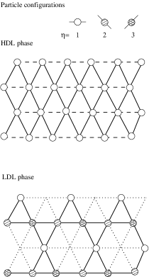
Figure 1: A representation of the two ordered phases of the model with the configuration of each particle identified by the orientation of the inert arms (upper panel). In both high density liquid (middle panel) and low density liquid phases (bottom panel) hydrogen bonds are indicated using full lines lattice edges with van der Waals interactions only are drawn with dashed lines, while the other lattice edges are represented by dotted lines.

To describe the sublattice structure of the LDL phase it is necessary to introduce four sublattices: three of them formed by sites on the borders of the hexagons and the central sites (see Fig. 2 (a)). This immediately leads to a fourfold degeneracy (corresponding to the placement of a hole in four different sites), which is captured by the Husimi tree if the homogeneity assumption is avoided (p09 ). The sublattices are equivalent in the HDL but we take care of the orientational order. This leads to a threefold degeneracy (corresponding to possible orientations for water molecules in the lattice), and this behavior is also captured by the tree without the homogeneity assumption. As will be shown later, the states of the central site of each hexagonal plaquette will always be summed in the recursive equations obtained from the hierarchical structure of the lattice. Considering this (and also to simplify our notation), we use only the three sublattices for the sites on the perimeters of the hexagons, as is shown in Fig. 2.

Let us now discuss the ground state of the model in some detail. In the GAS phase all sites are empty and we will associate a vanishing energy to this configuration, $E_{GAS}=0$. The LDL phase on the Husimi lattice is fourfold degenerate, characterized by empty sites either at the center of each hexagon or at the sites of one of the three sublattices A, B, and C. Recalling that all edges between first neighbor sites occupied by particles have hydrogen bonds on them, the energy per hexagon (including the chemical potential term) will be:

$$E_{LDL}=6(\epsilon+\gamma)-3\mu,$$ (1)

where we remember that each particle on the vertices of the hexagons is shared by two plaquettes. In the HDL phase, all sites are occupied and 8 of the 12 edges of each hexagon are occupied by hydrogen bonds, while the remaining 4 are not. Thus, there are three possible configurations of the hydrogen bonds. The energy per hexagon in this phase is:

$$E_{HDL}=12\epsilon+8\gamma-4\mu.$$ (2)

It is easy to find which phase corresponds to the minimum energy for given parameters $\epsilon$, $\gamma$, and $\mu$. Using the vdW interaction $\epsilon$ as the energy scale, we may define the dimensionless variables ${\bar{\gamma}}=|\gamma|/\epsilon$ and ${\bar{\mu}}=\mu/\epsilon$. The ground state corresponds to the GAS phase if ${\bar{\mu}}<2(1-{\bar{\gamma}})$, to the LDL phase if $2(1-{\bar{\gamma}})<{\bar{\mu}}<2(3-{\bar{\gamma}})$, and to the HDL if ${\bar{\mu}}>2(3-{\bar{\gamma}})$. As observed above, these values are the same as the ones found for the ground state on the triangular lattice b07 .

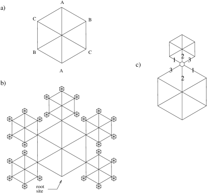
Figure 2: a) Definition of the sublattices. b) A subtree with three generations. c) Definition of $\eta$ for a site occupied by a particle. The numbers on the lattice edges correspond to the values of the variable $\eta$ if the inert bonds of the particle are placed on these edges.

II.1 Recurrence relations on the Husimi cactus

As usual, we start defining partial partition functions for rooted subtrees, fixing the configuration of the root. One of these subtrees is shown in Fig. 2. There are $3\times 4$ configurations of the root sites, so we define 12 partial partition functions $g_{i}$, $i=1,2,\ldots,12$, where the index $i$ stands for the root site configuration. We may associate the configurations $(s,\eta)$, where $s=A,B,C$ stands for the sublattice and $\eta=0,1,2,3$ for the site configuration, to the indices $i$ of the partial partition functions following the convention indicated in table 1. It is also useful to define the configurations of the bonding arms of a particle in a way which may be applied to all sites of the tree (only sites at the perimeter of the hexagons are considered, since we will sum over the configurations of the central sites). We therefore consider a particular site with a particle on it, which will belong to two hexagons in different generations of the tree, and imagine that we circle around the site clockwise, starting outside the hexagons. The configuration variable $\eta$ associated to this site will be equal to the number of lattice edges we cross until the one where one of the inert arms of the particle are located is reached, added with one. This definition is illustrated in Fig. 2. We proceed considering the operation of attaching 5 subtrees with $M$ generations to a new root hexagon, building a subtree with $M+1$ generations. Summing over the $4^{5}=1024$ possible configurations of the root sites of the $M$-generations subtree, we will arrive to recursion relations for the partial partition functions, which are of the form:

$$g_{i}^{M+1}=\sum_{j=1}^{1024}\left(\sum_{k=0}^{3}z^{n_{j,k}}\omega_{p}^{p_{i,j,k}}\omega_{b}^{b_{i,j,k}}\right)\prod_{\ell=1}^{12}(g_{\ell}^{M})^{e_{i,j,\ell}},$$ (3)

where $n_{j,k}$, $p_{i,j,k}$, and $b_{i,j,k}$ are the number of particles, number of pairs of particles in first neighbor sites and number of hydrogen bonds for each contribution $j$ to the partial partition function of $g_{i}^{M+1}$, given that the configuration $\eta$ of the central site is equal to $k$. $\omega_{p}=\exp[-\epsilon/(k_{B}T)]$ and $\omega_{b}=\exp[-\gamma/(k_{B}T)]$ are the Boltzmann factors associated to the van der Waals interactions and hydrogen bonds, respectively. We notice that the activity of the particle which eventually is placed on the root site is not considered at this level. The exponents $e_{i,j,\ell}$ assume integer values between 0 and 2. We remark that for each pair of indices $(i,j)$ there will be at most five nonzero exponents $e_{i,j,\ell}$, since this is the number of subtrees with $M$ generations linked to the new hexagon at the root. The exponents $e_{i,j,\ell}$ depend of the index $i$ only because the number of incident subtrees with root sites in each sublattices depends of the sublattice of the root site of the new subtree.

$(s,\eta)$	$i$	${\bar{i}}$
$(A,1)$, $(A,2)$, $(A,3)$	$1$, $2$, $3$	$10$
$(B,1)$, $(B,2)$, $(B,3)$	$4$, $5$, $6$	$11$
$(C,1)$, $(C,2)$, $(C,3)$	$7$, $8$, $9$	$12$
$(A,0)$, $(B,0)$, $(C,0)$	$10$, $11$, $12$	$-$

Table 1: To each possible state of a site, specified by its sublattice $s$ and configuration $\eta$ (first column), an index $i$ is assigned (second column). The indexes ${\bar{i}}$ which appear in the denominator of eq. (4) are shown on the third column.

In similar calculations, often the recursion relations are obtained by hand, usually summing the contributions with some graphical aid. In the present case, due to the large number of contributions, this procedure is very tedious and therefore errors are quite frequent. Although we actually obtained the recursion relations explicitly in this way, using symmetries to generate the expressions for the recursion relations, these expressions are much too large to be given here. To assure that the recursion relations are free of errors, we also decided to write a rather simple code which generates the sets of 24 integer numbers $n_{j,k}$, $p_{i,j,k}$, $b_{i,j,k}$ and $e_{i,j,\ell}$ for each contribution $j$ to the recursion relation for $g_{i}^{M+1}$, similar to what was done by Zara and Pretti in a model for RNA on the Husimi lattice z06 . Since we are interested in the behavior of the model in the thermodynamic limit, we should consider fixed points of these recursion relations. As expected, however, the partial partition functions diverge in this limit. So, we may define ratios of these functions, which may approach a finite value as $M\to\infty$. We thus define the ratios $R_{i}$, $i=1,2,\ldots,9$, dividing each partial partition function with a particle at the root site by the partial partition function with an empty root site in the same sublattice. This leads us to the ratios $R_{i}=g_{i}/g_{\bar{i}}$, where the values of ${\bar{i}}$ are shown in table 1. We may then obtain recursion relations for the ratios from the ones for the partial partition functions, Eq. 3. They are:

$$R_{i}^{M+1}=\frac{\sum_{j=1}^{1024}\left(\sum_{k=0}^{3}z^{n_{j,k}}\omega_{p}^{p_{i,j,k}}\omega_{b}^{b_{i,j,k}}\right)\prod_{\ell=1}^{9}(R_{\ell}^{M})^{e_{i,j,\ell}}}{\sum_{j=1}^{1024}\left(\sum_{k=0}^{3}z^{n_{j,k}}\omega_{p}^{p_{{\bar{i}},j,k}}\omega_{b}^{b_{{\bar{i}},j,k}}\right)\prod_{\ell=1}^{9}(R_{\ell}^{M})^{e_{{\bar{i}},j,\ell}}}.$$ (4)

II.2 Densities in the core of the Husimi cactus

In order to obtain densities in the central region of the tree, we consider the operation of attaching 6 subtrees to the central hexagon, which leads to an expression for the partition function of the whole tree:

$$Y_{M}=\sum_{j=1}^{4096}\left(\sum_{k=0}^{3}z^{N_{j,k}}\omega_{p}^{P_{j,k}}\omega_{b}^{B_{j,k}}\right)\prod_{\ell=1}^{12}(g_{\ell}^{M})^{E_{j,\ell}},$$ (5)

where $N_{j,k}$, $P_{j,k}$ and $B_{j,k}$ are the total number of particles, nearest neighbors and hydrogen bonds on the central hexagon with the configuration of the border sites given by $j$ and the central site in the configuration $k$, and $E_{j,\ell}$ is the number of border sites with configuration $\ell$.

Again the set of integer exponents was generated by a computer program, as well as manually, and both procedures lead to the same final results. Now, for example, the density of particles (defined here as the number of particles divided by the number of sites) in the central hexagon will be given by:

$$\rho=\frac{z}{7Y_{M}}\frac{\partial Y_{M}}{\partial z},$$ (6)

where $\rho$ is in the range $[0,1]$. We notice that the activities of the sites at the perimeter and the center of the central hexagon of the tree are considered in expression (5), so the factor 7 assures the proper normalization of the density. In other words, the numbers $N_{j,k}$ in expression (5) are in the range $[0,7]$. A similar procedure leads to expressions for the densities of hydrogen bonds and van der Waals interactions per site. Dividing both the numerator and the denominator of the expressions for the densities by $(g_{10}^{M}\,g_{11}^{M}\,g_{12}^{M})^{2}$ we may express them in terms of the ratios and the parameters of the model. Thus, for example:

$$\rho=\frac{1}{7}\frac{\sum_{j=1}^{4096}\left(\sum_{k=0}^{3}N_{j,k}z^{N_{j,k}}\omega_{p}^{P_{j,k}}\omega_{b}^{B_{j,k}}\right)\prod_{\ell=1}^{9}(R_{\ell}^{M})^{E_{j,\ell}}}{\sum_{j=1}^{4096}\left(\sum_{k=0}^{3}z^{N_{j,k}}\omega_{p}^{P_{j,k}}\omega_{b}^{B_{j,k}}\right)\prod_{\ell=1}^{9}(R_{\ell}^{M})^{E_{j,\ell}}}.$$ (7)

To obtain the thermodynamic behavior of the model, we may iterate the recursion relations until a fixed point for the ratios $R_{\ell}$ is reached with the required numerical precision, and then calculate the densities at the center of the tree. The convergence of the recursion relations generally is quite fast. In certain regions of the parameter space, more than one fixed point may be stable, signaling coexistence of phases. To locate the first order transition in such cases it is necessary to compare free energies of different phases. An expression for the grand-canonical free energy is obtained in what follows.

II.3 Grand-canonical free energy

To obtain the grand-canonical free energy of the model in the core of the tree, we may proceed following the prescription proposed by Gujrati g95 . For this purpose, it is convenient to notice that if we connect the central site of each hexagon to the central sites of the first-neighbor hexagons, we end up with a Cayley tree with coordination $q=6$ and ramification $\sigma=q-1=5$. Now we may assume that the total free energy of the tree is the sum of the free energies associated to each hexagon. This takes care of the sublattice structure of the model. The hexagons may then be classified in generations identified by the index $m$, starting with the ones placed on the surface, for which $m=1$ and ending at the central site ($m=M$ for a tree with $M$ generations of hexagons). It is natural, considering the structure of the tree, to assume a radial symmetry for the local free energies, so that we will represent by $\phi_{M}(m)$ the free energy of a hexagon in the $m$’th generation of a tree with a total of $M$ generations. The total free energy of the tree will then be:

$$\Phi_{M}=\sum_{m=1}^{M}N_{M}(m)\phi_{M}(m),$$ (8)

where $N_{M}(M)=1$ and

$$N_{M}(m)=q\sigma^{M-m-1},\;\;m=1,2,\ldots,M-1$$ (9)

are the numbers of hexagons in the $m$’th generation. Now we may see that:

$$\Phi_{M+1} - \sigma\Phi_{M}=\phi_{M+1}(M+1)-\sigma\phi_{M}(M)+q\phi_{M+1}(M)$$ (10)

$$+q\sum_{m=1}^{M}\sigma^{M-m}[\phi_{M+1}(m)-\phi_{M}(m)].$$

It is now reasonable to assume that in the thermodynamic limit we should have the free energies per hexagon in the core of the tree approaching a limiting bulk value $\phi_{b}$, so that $\phi_{M+1}(M+1)=\phi_{M}(M)=\phi_{M+1}(M)=\phi_{b}$ for $M\to\infty$. Close to the surface, the free energies per hexagon should be functions of $m$, but we may assume $\phi_{M+1}(m)-\phi_{M}(m)\to 0$ when $M\to\infty$. Therefore, we may conclude from equation (10) that:

$$\phi_{b}=\frac{1}{2}(\Phi_{M+1}-\sigma\Phi_{M}),$$ (11)

in the thermodynamic limit $M\to\infty$ and for the model we are considering here $\sigma=5$. Actually, this expression may also be obtained from a somewhat stronger assumption that the free energies per hexagon in the thermodynamic limit should assume only two values: $\phi_{b}$ on the surface $m=1$ and $\phi_{b}$ in all other cases oss09 . Also, we notice that the original argument for the calculation of the free energy was also recently generalized for Husimi trees with a sublattice structure in Semerianov and Gujrati sg05 . The derivation presented here is different from the ones originally proposed in g95 and sg05 , but the results are the same footn02 .

Since the partition function on a $M$-generations tree is $Y_{M}$, we have:

$$\phi_{b}=-\frac{1}{2}k_{B}T\ln\left(\frac{Y_{M+1}}{Y_{M}^{5}}\right).$$ (12)

Substituting the partition function (5) in this expression, and expressing the sums in terms of the ratios, we obtain:

$$\frac{Y_{M+1}}{Y_{M}^{5}}=\frac{1}{\left[\sum_{j=1}^{4096}\left(\sum_{k=0}^{3}z^{N_{j,k}}\omega_{p}^{P_{j,k}}\omega_{b}^{B_{j,k}}\right)\prod_{\ell=1}^{9}(R_{\ell}^{M})^{E_{j,\ell}}\right]^{4}}\times\frac{(g_{10}^{M+1}g_{11}^{M+1}g_{12}^{M+1})^{2}}{(g_{10}^{M}g_{11}^{M}g_{12}^{M})^{10}}.$$ (13)

Now we may use the recursion relations Eqs. (3) to express the partial partition functions for subtrees with $M+1$ generations in terms of the ones with $M$ generations, and finally will arrive at the expression for the second fraction in expression (13)

$$\frac{(g_{10}^{M+1}g_{11}^{M+1}g_{12}^{M+1})^{2}}{(g_{10}^{M}g_{11}^{M}g_{12}^{M})^{10}}=\prod_{i=10}^{12}\left[\sum_{j=1}^{1024}\left(\sum_{k=0}^{3}z^{n_{j,k}}\omega_{p}^{p_{i,j,k}}\omega_{b}^{b_{i,j,k}}\right)\prod_{\ell=1}^{9}(R_{\ell}^{M})^{e_{i,j,\ell}}\right]^{2}.$$ (14)

Therefore, we see that we may express the bulk free energy per hexagon as a function of the parameters of the model and the ratios $R_{i}$, and in the thermodynamical limit it will converge to a fixed point value. Finally, since we are in the grand-canonical ensemble, we have that the pressure is $P=-\Phi/V$, where $\Phi$ is the grand-canonical potential and $V$ the volume. Associating a volume $v_{0}$ to each site of the lattice and recognizing $\phi_{b}$ as the grand-canonical potential per hexagon for the solution on the Husimi tree, the pressure may be written as

$$P=-\phi_{b}/{4v_{0}},$$ (15)

where it should be stressed that we have four sites per hexagon in the core of the tree.

III Thermodynamical behavior of the model

To study the thermodynamical behavior of the model on the Husimi lattice, we define reduced intensive or fieldlike thermodynamic variables (temperature, pressure and chemical potential) as ${\bar{T}}=k_{B}T/\epsilon$, ${\bar{\mu}}=\mu/\epsilon$ and ${\bar{P}}=Pv_{0}/\epsilon$. Considering expressions (12) and (15), the reduced pressure is given by:

$${\bar{P}}={\bar{T}}\frac{\ln\left(\frac{Y_{M+1}}{Y_{M}^{5}}\right)}{8}.$$ (16)

As mentioned before, we limited our study on the particular case ${\bar{\gamma}}=2$, for which MC simulations were found in the literature. For fixed values of ${\bar{T}}$ and ${\bar{\mu}}$, we iterate the recursion relations (4) for the ratios of partial partition functions, and once the fixed point is reached, we determine the mean numbers of particles, hydrogen bonds and van der Waals interactions per lattice site, which are represented by $\rho$, $\nu_{hb}$, and $\nu_{vW}$, respectively. The densities of hydrogen bonds and van der Waals interactions per site, normalized to be in the range $[0,1]$, will be $\rho_{HB}=\nu_{HB}/2$ and $\rho_{vW}=\nu_{vW}/3$. Finally, the pressure may be also obtained at the fixed point.

The phase diagram of the model was found using this procedure, being presented in the $({\bar{T}},{\bar{P}})$ plane on Fig. 3. The three phases used in our ground state analysis were also found at finite temperature and coexistence lines between these phases were calculated by requiring the identity of their bulk free energies. All transitions are discontinuous and a triple point, located at ${\bar{P}}=2.997$, ${\bar{T}}=0.835$, and ${\bar{\mu}}=1.959$, was found. The coexistence lines meeting at the triple point satisfy the thermodynamical requirements for this situation, such as the 180 degree rule w74 .

Figure 3: (color on line) a) Phase diagram (${\bar{T}}\times{\bar{P}}$) of the Henriques-Barbosa model on the Husimi lattice, as defined on section II. Dashed lines are discontinuous transitions which meet at triple point represented by a full circle (red on-line). The full lines are the stability limits of the GAS (no symbol, red on line), LDL (squares, blue on line), and HDL (triangles, green on line) phases. The dotted and dash-dotted lines (black on line) are the TmD and TMD, respectively. b) A detail of Fig. a) where the lines of density anomalies are more visible. c) Present results for the coexistence lines and triple point are compared to the first order phase transitions (circles) and TMD (triangles) from Monte Carlo simulations of Balladares et al b07 .

Our phase diagrams are qualitatively different from the one originally suggested based on Monte Carlo simulations b07 , where the two coexistence lines start at low temperatures and end at critical points. They are also different from the cluster variational results obtained for several waterlike models on the $bcc$ latticebs08 ; p09 , where the coexistence lines end at tricritical points. In Fig. 3(c) the MC simulation results presented in b07 are also shown and a good agreement on the location of the phase transitions is found between those and our results, except on the low-temperature region of the LDL-HDL coexistence line. Along this region the simulations present a rather large positive slope, and since the ground-state value is exactly known (${\bar{P}}=3$), a large negative slope should occur in the LDL-HDL coexistence line at low temperatures. This effect is even enhanced if we recall that, due to the third law of thermodynamics and the Clausius-Clapeyron equation, the coexistence curve has to be horizontal at vanishing temperature footn03 . A similar situation was found in the simulations of the model with distinction between donor and acceptor arms h05 , where this point is discussed, particularly with respect to the implications of the Clausius-Clapeyron relation. Although these simulations have been recently revisited s09 , the new results for the LDL-HDL coexistence line do not include temperatures low enough to reach the region we are discussing here. In our calculation, the HDL-LDL coexistence curve starts with zero slope at vanishing temperature. As the temperature increases, the slope has a small positive value, then the curve presents a maximum and the slope becomes negative close to the triple point. These features are not visible in the scale of Fig. 3. It is interesting to notice that the estimated location for the LDL-HDL critical point in the simulations is quite close to the triple point in our solution.

We carefully verified if the transitions are actually discontinuous by studying the stability limits of the fixed points associated to each phase. These limits may be found calculating the jacobian of the recursion relations (4)

$$J_{i,j}=\left(\frac{\partial R_{i}^{M+1}}{\partial R_{j}^{M}}\right),$$ (17)

at the fixed point ($M\to\infty$), and then requiring the absolute value of the largest eigenvalue of the jacobian to be equal to one. In Fig. 3(a) the stability limits of all phases are shown. Although in part of the GAS-LDL coexistence line the stability limit of the LDL phase is very close to the transition, they are never coincident, thus assuring the discontinuity of the transition.

In order to find out if the stability limits of the fixed points are in fact the spinodals (thermodynamic stability limits), we also calculated the eigenvalues of the hessian associated with the phases. For the ordered phases (LDL and HDL) we found a good numerical coincidence of the spinodals and the stability limits everywhere. For the GAS phase, at low temperatures, we were able to assure numerically the coincidence between these curves, but at higher temperatures we had numerical problems to evaluate the elements of the hessian, which are second derivatives of the potential.

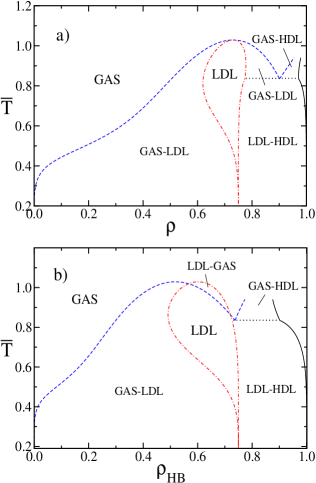
Figure 4: (color on line) Temperature $\times$ density diagrams. a) Particle density. b) Hydrogen bond density. The temperature of the triple point is indicated by a dashed line. Densities of the phases at coexistence are indicated. The full line (black on line) corresponds to the HDL phase, the dashed line (blue on line) to the GAS phase and the dot-dashed line (red on line) the the LDL phase. The dotted horizontal line corresponds to the three-phase coexistence (triple point).

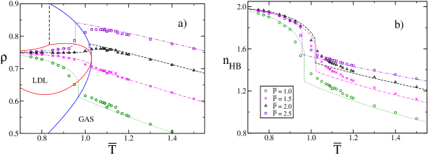
Figure 5: (color on line) Isobaric curves of densities as a function of temperature. Broken lines are the results obtained in this work, with the vertical tielines also indicated at coexistence. Symbols are results from simulations by Balladares et al b07

An interesting point is that the LDL-GAS coexistence line has two regions with slopes of different signs, showing a reentrant behavior. The ${\bar{\mu}}\times{\bar{T}}$ phase diagram is quite similar to the ${\bar{P}}\times{\bar{T}}$ phase diagram shown in Fig. 3. The change of the sign happens at a point which is located at ${\bar{\mu}}_{max}=0.137$, ${\bar{T}}_{max}=1.029$, and ${\bar{P}}_{max}=1.686$. Since the GAS phase has a larger entropy at the coexistence with the LDL phase, the Clausius-Clapeyron relation indicates that the particle density should be lower for the GAS phase than for the LDL phase in the part of the coexistence curve with pressures lower than ${\bar{P}}_{max}$. At $({\bar{T}}_{max},{\bar{P}}_{max})$, the densities of both phases are identical and in the remainder of the coexistence the density of the GAS phase is higher. In fact, the equal densities at this point are confirmed in Fig. 4(a), where the temperature is shown as a function of the density of particles at coexistence. It is important to remind that GAS and LDL phases are not identical on this point (in this case it would be a critical point). As can be observed in the phase diagram with the density of hydrogen bonds, instead of the particle density, shown in Fig. 4(b). Although not presented here, densities of vdW interactions are also different for both phases on this point.

Another relevant question is the location of the points of maximum density in the isobars. We found that isobars for the densities of particles as functions of the temperature do actually present a maximum at pressures above ${\bar{P}}_{max}$. This TMD is located in the metastable extension of the GAS phase inside the LDL phase, in Figs. 3(a) and 3(b), we represented the location of these metastable TMD of the GAS with the dash dotted line. It ends at the point of maximum temperature of the GAS spinodal, as may be seen in the detail (Fig. 3(b)). We also found a temperature of minimum density line (TmD) inside the LDL phase, shown in Figs. 3(a) and (b) as a dotted line. This line occurs also at pressures higher than ${\bar{P}}_{max}$ and, unlike the TMD, which is located in the metastable GAS phase, the TmD line covers both stable and metastable regions of the LDL, ending at the point of maximum temperature of the LDL spinodal, a detail also more visible in Fig. 3(b). It is actually expected that lines of vanishing thermal expansion coefficient should end at the points where the corresponding spinodals change the sign of their slope s82 . Finally, it should be mentioned that similar findings were reported by Pretti and Buzzano in their homogeneous cluster variational study of the symmetric Roberts-Debenedetti model p04 .

In Fig. 5 we show some isobars for the densities of particles and hydrogen bonds. The results of the present calculations are represented by the broken lines, and the symbols close to the isobars are the MC simulation results obtained by Balladares et al b07 . We notice a good quantitative agreement between them and our calculations, at least not too close to the coexistence line. In the ${\bar{P}}\times{\bar{T}}$ diagram shown in Fig. 3(c), the locations of the TMD points found in the simulations presented in b07 are represented by triangles, and in general we may notice that they are located at temperatures larger than the ones of coexistence. These estimates actually correspond to the maxima in the density at the coexistence curve, and the fact that they lie above the coexistence curve may be due to finite-size effects. As another possibility, the Bethe lattice approximation introduced here could underestimate the location of the TMD due to the absence of a LDL-GAS critical transition, observed in simulations, at least for the model with distinction between donors and acceptors s09 . In principle, the presence of such a critical line could increase the entropy-volume cross fluctuations and shift the TMD line ($Vk_{B}T\alpha=\langle\delta V\delta S\rangle=0$) to higher temperatures. For example, this kind of TMD underestimation happened in Bethe lattice solution of the Bell-Lavis model of liquid water b08 , when compared to Monte Carlo simulations f09 .

In Fig. 5(b) the mean number of hydrogen bonds per particle ($n_{HB}=\nu_{HB}/\rho=2\rho_{HB}/\rho$) is depicted at constant pressure as a function of the temperature. Again, a good quantitative agreement between our results and the MC simulations was found. In the simulations, crossing of different isobars was reported and its physical origin was discussed b07 , in relation to density anomaly. Nevertheless, our calculations suggest the possibility of the crossing being a consequence of the discontinuous transition between the LDL and GAS phases and finite-size rounding effects in the isobars.

IV Final discussion and conclusion

In this paper we solved the Henriques-Barbosa model with symmetric arms b07 on a Husimi lattice built with hexagons. Two liquid and one gas phase are present in the phase diagram, but qualitative differences are found when compared with the phase diagram which was obtained with simulations. All transitions we found are discontinuous, and also a triple point was found where all phases coexist with different densities. We carefully checked if the transitions are really discontinuous, since in part of the coexistence loci the discontinuities are rather small. Thus we assured that the stability limits of the fixed points associated to the coexisting phases are never coincident. Also, it may be seen in Figs. 4 that the densities present a discontinuity at the coexistence line, although it may be rather small, particularly in the neighborhood of the point of maximum temperature in the GAS-LDL coexistence line.

Recently, more detailed simulations were reported on this model with distinction between donor and acceptor arms s09 , and a diagram closer to the one we present here was found. The difference is that the GAS-LDL transition line is discontinuous at low temperatures, but becomes a critical line when the temperature is increased, thus a tricritical point is present. Also, the HDL-GAS transition appears to be continuous in the new simulations. The LDL-HDL line is always discontinuous, so that in the simulations the point which corresponds to the triple point in our phase diagrams appears as a bicritical point (which was called wrongly as a tricritical point in the caption of Fig. 3 in reference s09 ). Nevertheless, a direct comparison between the present calculation and these new simulations may not be done, since the distinction between donor and acceptor arms leads to an increase of the entropy of the model. It is not impossible that a transition found to be discontinuous in mean-field like approximations turns out to be continuous in simulations or more precise calculations, such as series expansions. However, we notice that the results of the calculations presented here show, in general, good agreement with data furnished by simulations, as was also noticed by Buzano and collaborators in their study of an associating lattice gas model, with tetragonal symmetry, on the $bcc$ lattice bs08 . It is worth mentioning that the phase behavior presented by the most recent simulations of the Henriques-Barbosa model is different from that found for the associating lattice gas model studied with the cluster variational method on Ref. bs08 . There, instead of a bicritical point, a tricritical and a critical endpoint are present. We are presently studying this model with the same methods implemented on this paper.

Although the results presented here for the coexistence lines in the pressure-temperature phase diagram agreed well with the data of simulations in b07 , this is not the case for the low-temperature region of the LDL-HDL coexistence curve, where the simulations suggest a minimum while a smooth behavior was found in our results. The interpretation of this apparent minimum in relation with the Clausius-Clapeyron equation seems unclear to us, and we believe on the possibility that these results might be spurious. Possibly, longer equilibration times for MC simulations should be considered on this low-temperature region.

If we adopt the qualitative phase diagram which emerges from our calculations, the TMD found in the simulations would correspond to the coexistence line. Nevertheless, it is also possible that the absence of a critical line results in an overall decrease of the temperatures of the TMD line, as in the case of the Bell-Lavis model b08 ; f09 . The crossing of isobaric curves for the density of hydrogen bonds as function of the temperature was observed in the simulations, but here it may be seen as a consequence of rounding finite size effects for the discontinuous transition at the LDL-GAS coexistence curve, with no relation to the TMD. The LDL-GAS coexistence curve actually is a very weak discontinuous transition in the region where the simulations suggested the presence of a critical point. This indicates that the question of the order of the transition in this region should be studied very carefully in simulations.

The results presented here support that the phase diagram of the symmetric Henriques-Barbosa model does not present a second critical point, as originally suggested through Monte Carlo simulations b07 . Our theoretical phase diagram is actually closer to the results of more recent simulation of a original (asymetrical) model s09 : phase transitions are found in both cases, but second order transitions are not present in our theoretical results, this may be due to the limitation of the Husimi lattice solution to capture long-range correlations.

Considering the technical aspects of the Husimi lattice, our calculation shows the importance of a careful choice of the sublattice structure to capture the correct phase diagram of not so simple lattice models. A simpler homogeneous lattice structure would lead the system to thermodynamic states which may be unstable or metastable in the more general parameter space used here (results not shown). On this sense, it is worth mentioning that usually the simplest choice for the plaquette in Husimi lattice calculations to approximate the behavior of models on regular lattices is the elementary polygon in the original lattice. Therefore, the simplest choice in the present case would be a Husimi lattice with triangular plaquettes and coordination number equal to 6. However, such a choice would probably not lead to results comparable to the ones obtained in simulations. The rather unusual choice of plaquettes we adopted here is certainly responsible for the good quantitative agreement between our results and the simulations. This technical discussion is extremely relevant to the subject since one can find in the literature lattice models presenting water like behavior (including thermodynamic anomalies and interesting phase diagrams) which were studied without a more detailed sublattice analysis f02 ; c08 .

We finish remarking that many lattice models proposed to investigate waterlike anomalous behavior were found to present phase diagrams which were more complex than originally expected. When sublattice ordering is properly considered p09 , even the simplest models do present at least a single critical line, and many of them do not present gas-liquid phase transition ending in a critical point or a temperature of maximum density in a stable disordered fluid without a sublattice structure. The arbitrary use of the homogeneneity assumption can result in some interesting phase diagrams but, in our opinion, this assumption is an artifact which eventually may hide the instability of the homogeneous phase at low temperatures. Thus, this homogeneous solution could not be considered as a true implementation for a random lattice useful for representing fluids, as recently proposed p09 . Considering the results obtained here and in other recent papers bs08 ; p09 , the issue of finding a simple lattice model with minimal waterlike behavior seems to be far from being resolved. Monte Carlo simulations are certainly needed to determinate the ‘exact’ phase diagram but it seems that a modeling breakthrough will be needed to achieve a better description of liquid water.

References

- (1) G. R. Andersen and J. C. Wheeler, J. Chem. Phys. 69, 2082 (1978).
- (2) B. C. McEwan, J. Chem. Soc. 123, 2284 (1923).
- (3) R. R. Parvatiker and B. C. McEwan, J. Chem. Soc. 125, 1484 (1924).
- (4) J. Hirschfelder, D. Stevenson, and H. Eyring, J. Chem. Phys. 5, 896 (1937).
- (5) J. A. Barker and W. Fock, Disc. Faraday Soc. 15, 188 (1953).
- (6) J. C. Wheeler, J. Chem. Phys. 62, 433 (1975).
- (7) P. G. Debenedetti, J. Phys.: Cond. Matter 15, R1669 (2003).
- (8) P. H. Poole, F. Sciortino, U. Essmann, and H. E. Stanley, Nature 360, 324 (1992).
- (9) S. Harrington, R. Zhang, P. H. Poole, F. Sciortino, and H. E. Stanley, Phys. Rev. Lett. 78, 2409 (1997).
- (10) Y. Katayama, T. Mizutani, W. Utsumi, O. Shimomura, M. Yamakata, and K. Funakoshi, Nature 403, 170 (2000).
- (11) R. Kurita and H. Tanaka, Science 306, 845 (2004).
- (12) R. Kurita and H. Tanaka, J. Phys.: Cond. Matter 17, L293 (2005).
- (13) H. Tanaka, R. Kurita, and H. Mataki, Phys. Rev. Lett. 92, 025701 (2004).
- (14) J. R. Errington and P. G. Debenedetti, Nature 409, 318 (2001).
- (15) R. Sharma, S. N. Chakraborty, and C. Chakravarty, J. Chem. Phys. 125, 204501 (2006).
- (16) M. S. Shell, P. G. Debenedetti, and A. Z. Panagiotopoulos, Phys. Rev. E 66, 011202 (2002).
- (17) L. Xu, P. Kumar, S. V. Buldyrev, S.-H. Chen, P. H. Poole, F. Sciortino, and H. E. Stanley, Proc. Natl. Acad. Sci. 102, 16558 (2005).
- (18) P. Kumar, S. V. Buldyrev, S. R. Becker, P. H. Poole, F. W. Starr, and H. E. Stanley, Proc. Natl. Acad. Sci. 104, 9575 (2007).
- (19) G. M. Bell and D. A. Lavis, J. Phys. A 3, 568 (1970).
- (20) C. Buzano, E. De Stefanis, A. Pelizzola, and M. Pretti, Phys. Rev. E 69, 061502 (2004).
- (21) V. B. Henriques and M. C. Barbosa, Phys. Rev. E 71, 031504 (2005).
- (22) S. Sastry, F. Sciortino, and H. E. Stanley, J. Chem. Phys. 98, 9863 (1993).
- (23) G. Franzese and H. E. Stanley, Physica A 314, 508 (2002).
- (24) G. M. Bell, J. Phys. C 5, 889 (1972).
- (25) N. A. M. Besseling and J. Lyklema, J. Phys. Chem. B 101, 7604 (1997).
- (26) C. J. Roberts and P. G. Debenedetti, J. Chem. Phys. 105, 658 (1996).
- (27) M. Pretti and C. Buzano, J. Chem. Phys. 121, 11856 (2004).
- (28) M. Girardi, A. L. Balladares, V. B. Henriques, and M. C. Barbosa, J. Chem. Phys. 126, 064503 (2007).
- (29) P. Kumar, G. Franzese, and H. E. Stanley, Phys. Rev. Lett. 100, 105701 (2008).
- (30) M. M. Szortyka and M. C. Barbosa, Physica A 380, 27 (2007).
- (31) M. Girardi, M. M. Szortyka, and M. C. Barbosa, Physica A 386, 692 (2007).
- (32) V. B. Henriques and M. C. Barbosa, private communication.
- (33) V. B. Henriques, N. Guisoni, M. A. A. Barbosa, M. Thielo, and M. C. Barbosa, Mol. Phys. 103, 3001 (2005).
- (34) A. L. Balladares, V. B. Henriques, and M. C. Barbosa, J.Phys.: Cond. Matter 19, 116105 (2007).
- (35) M. A. A. Barbosa and V. B. Henriques, Phys. Rev. E 77, 051204 (2008).
- (36) C. Buzano, E. De Stefanis, and M. Pretti, J. Chem. Phys. 129, 024506 (2008).
- (37) M. Pretti, J. Stat. Phys. 111, 993 (2003).
- (38) M. Pretti, C. Buzano, and E. De Stefanis, J. Chem. Phys. 131, 224508 (2009).
- (39) M. M. Szortyka et. al., J. Chem. Phys. 130, 184902 (2009).
- (40) P. D. Gujrati, Phys. Rev. Lett. 74, 809 (1995).
- (41) A typo in the expression (2) of reference b07 should be corrected: the factor before the second sum should be replaced by .
- (42) R. A. Zara and M. Pretti, Physica A 371, 88 (2004).
- (43) T. J. Oliveira, J. F. Stilck, and P. Serra, Phys. Rev. E 80, 041804 (2009).
- (44) F. Semerianov and P. D. Gujrati, Phys. Rev. E 72, 011102 (2005).
- (45) In sg05 a model is solved on the Husimi lattice built with squares such that at each site of the tree two squares of successive generations are connected. The ramification of the Cayley tree built by connecting the centers of the squares is and therefore the bulk free energy per square will be . If we now remember that we have two sites per square in this lattice, the free energy per site is equal to , which, adapting the notation, corresponds exactly to expression (A7) for this quantity in sg05 .
- (46) J. C. Wheeler, J. Chem. Phys. 61, 4474 (1974).
- (47) This is not the case of systems which do present residual entropy. As an example, the model studied in ref. b08 displays a coexistence line with finite slope because the high density liquid has a residual entropy, whose origin is related to presence of frustration.
- (48) R. J. Speedy, J. Phys. Chem. 86, 982 (1982).
- (49) C. E. Fiore et al, J. Chem. Phys. 131, 164506 (2009).
- (50) G. Franzese and H. Eugene Stanley, Physica A 314, 508 (2002).
- (51) A. Ciach, W. Góźdź, and A. Perera, Phys. Rev E 78, 021203 (2008).