HST/NICMOS observations of the GLIMPSE9 stellar cluster.

Abstract

We present HST/NICMOS photometry, and low-resolution K-band spectra of the GLIMPSE9 stellar cluster. The newly obtained color-magnitude diagram shows a cluster sequence with $H$-K_S $=\sim 1$ mag, indicating an interstellar extinction A${}_{\rm K_{\rm s}}$$=1.6\pm 0.2$ mag. The spectra of the three brightest stars show deep CO band-heads, which indicate red supergiants with spectral type M1-M2. Two 09-B2 supergiants are also identified, which yield a spectrophotometric distance of $4.2\pm 0.4$ kpc. Presuming that the population is coeval, we derive an age between 15 and 27 Myr, and a total cluster mass of $1600\pm 400$ M_⊙, integrated down to 1 M_⊙. In the vicinity of GLIMPSE9 are several HII regions and SNRs, all of which (including GLIMPSE 9) are probably associated with a giant molecular cloud (GMC) in the inner galaxy. GLIMPSE9 probably represents one episode of massive star formation in this GMC. We have identified several other candidate stellar clusters of the same complex.

1. Introduction

An understanding of the mechanisms of formation and evolution of massive stars is of broad astronomical interest. Through mass-loss and supernova explosions, massive stars return a significant fraction of their masses to the interstellar medium (ISM), thereby chemically enriching and shaping the ISM. Being very luminous, they can be identified in external galaxies, providing spectrophotometric distance. Observational constraints on the formation and evolution of massive stars are, however, difficult to obtain due to the rarity of these objects and their location in the Galactic plane, where interstellar extinction can hamper their detection.

Massive stars can be identified by their ionizing radiation, which creates easily identifiable HII regions. Furthermore, since the majority of massive stars are born in clusters (Lada & Lada, 2003), they are also identified by locating young massive stellar clusters. Over the past decade, infrared and radio observations of the Galactic plane have revealed several hundred new HII regions, more than 50 new candidate supernova remnants (SNR) (Giveon et al., 2005; Helfand et al., 2006), and 1500 new candidate infrared stellar clusters (e.g. Bica et al., 2003; Mercer et al., 2005; Froebrich et al., 2007), which are often found in the direction of HII regions. Only a few of these infrared candidate clusters have been confirmed with spectro-photometric studies; the analysis is often restricted only to stellar clusters and does not include the cluster environment. A combined study of stellar clusters and their associated molecular clouds is a powerful tool to understand star formation. Clusters appear to form in large complexes (e.g. Smith et al., 2009). The temporal and spatial distribution of clusters varies from cloud to cloud (e.g. Homeier & Alves, 2005; Kumar et al., 2004; Clark et al., 2009a), indicating that external and internal triggers are both at work. Supernova explosions may trigger subsequent episodes of star formation in the same cloud. The presence of SNRs indicates that a cloud has already undergone massive star formation, and the study of stellar clusters associated with SNRs can shed light on the initial masses of the supernova progenitors, and therefore on the fate of massive stars.

By locating new HII regions, and young stellar clusters, we also obtain information on large scale Galactic structures. So far, we have only located clusters that reside in the near side of the Galaxy, with a few exceptions, e.g. W49 (Homeier & Alves, 2005). Many issues on Galactic structures are still open, e.g.  the exact number of spiral arms, the lack of star formation in the central 3 kpc, and the possible existence of a ring of massive star formation surrounding the central bar. Stellar clusters selected from infrared observations are promising tracers for Galactic studies because they sample a larger portion of the Galactic plane than those from optical surveys (Messineo et al., 2009; Davies et al., 2007; Figer et al., 2006; Clark et al., 2009b).

The candidate cluster number 9 in the list by Mercer et al. (2005) (hereafter, GLIMPSE9) is an ideal target to study the issues above mentioned, because it is located in projection on a GMC that hosts several HII regions, supernova remnants, and candidate clusters. So far, we know only of one other Galactic cluster associated with a SNR (Messineo et al., 2008). This complex is on the Galactic plane, at an heliocentric distance of $\sim 4.9$ kpc (Albert et al., 2006; Leahy et al., 2008), and longitude l=$\sim 23$^∘, and represents an episode of massive star formation in the direction of the inner Galaxy. Here we present a spectro-photometric study of the GLIMPSE9 cluster.

In Sect. 2, we present the available photometric and spectroscopic data, and the process of data reduction. The spectral analysis and color-magnitude diagram study are given in Sect. 3. Information about the parent GMC and other candidate stellar clusters are presented in Sect. 4. Finally, in Sect. 5 we summarize the results of our investigation.

2. Observation and data reduction

2.1. NICMOS/HST observations

Images were taken with NICMOS on board the HST on July 9, 2008 as part of the GO program 11545 (P.I. Ben Davies). Two fields were observed; one centered on the GLIMPSE9 cluster (RA= 18$\fh$34$\fm$09.89^s, DEC=-09$\fdg$14$\farcm$04.8^′′) and another located at (RA=18$\fh$34$\fm$12.76^s, DEC=-09$\fdg$12$\farcm$45.4^′′). The latter, which we call the control field, was imaged in order to study the background and foreground stellar population in the direction of the cluster. The location of the two fields is shown in Fig. 1. The NIC3 field of view (51.5^′′$\times$ 51.5^′′) covers the cluster to a radius roughly equal to two half light radii ($\sim$30^′′, as measured on 2MASS images).

Figure 1.— The greyscale above shows a 2MASS K_S-band image, while contours show 24 $\mu$m emission from MIPSGAL. Contour levels are 100, 200, 300, 400, and 500 MJy/sr. The two boxes indicate the location and size of the two NIC3 fields. Extended emission at a 5 $\sigma$ level is seen towards the field.

We used the NIC3 camera with the F160W and F222M broadband filters, and with the F187N and F190N narrowband filters. The fields were dithered by 5.07^′′  in a spiral pattern (6 positions). The STEP2 sequence of the MULTIACCUM readout mode with 13 reads was used for exposures with the F160W filter, giving an integration time of 19.94 s per exposure; the STEP8 sequence with 12 reads was used for exposures with the F222M filter (55.94 s), and the STEP8 with 10 reads for exposures with the F187N and F190N filters (39.95 s).

Figure 2.— Top: F160W mosaic of the GLIMPSE9 cluster. Squares and identification numbers (from Table 1) show the location of spectroscopically observed stars. Stars #10 and #11 fall outside the field of view. Bottom: F160W mosaic of the control field.

2.2. NICMOS/HST data reduction

The images were bias subtracted, dark corrected, and flat-fielded by the standard NICMOS pipeline CALNICA (see the NICMOS Data Handbook v7.0). The six dithered exposures of each observation were re-sampled into a final mosaic with a pixel scale of 0.066^′′. The cluster mosaics are shown in Fig.  2.

A major photometric uncertainty is inherent for images with the NIC3 camera, and is due to the combination of an under-sampled point spread function (PSF) with the lower intrapixel sensitivity of the camera (up to 10-20%, see the NICMOS Data Handbook v7.0). The dithering observing strategy reduces this uncertainty. A photometric analysis of the mosaics was carried out with DAOPHOT Stetson (1987) within the Image Reduction and Analysis Facility (IRAF). We used the images of the control field, which is less crowded, to build a point-spread-function (PSF); seven isolated and bright stars were selected in the F160W and F222M images. Due to the small number of isolated stars no attempt was made to model a spatially varying PSF. Aperture photometry with a radius of 1.1^′′ was performed on bright and isolated stars, and the average difference between these magnitudes and the PSF-fitting magnitudes from DAOPHOT was measured. This aperture correction was applied to the whole catalogue. We obtained calibrated magnitudes in the Vega system with the transformation equations between counts/s to Vega magnitudes as given in the NICMOS Data Handbook. Astrometry and photometric calibrations into the 2MASS system were obtained using a set of 13 point sources with good quality $H$ and $K_{S}$ measurements in 2MASS (Skrutskie et al., 2006). The reference stars span a $H-K_{S}$ range from 0.2 to 1.4 mag, and a $K_{S}$ range from 6.3 to 14.0 mag.

The transformation equations are:

$$K_{s}-[F222M]=~{}~{}~{}~{}~{}~{}~{}~{}~{}~{}~{}~{}~{}~{}~{}~{}~{}~{}~{}~{}$$

$$(-0.01\pm 0.10)+(-0.03\pm 0.08)\times([F160W]-[F222M]),$$

$$H-[F160W]=~{}~{}~{}~{}~{}~{}~{}~{}~{}~{}~{}~{}~{}~{}~{}~{}~{}~{}~{}~{}$$

$$(-0.08\pm 0.09)+(-0.22\pm 0.07)\times([F160W]-[F222M]),$$

with a standard deviation of 0.11, and 0.10 mag, respectively. $[F222M]$ and $[F160W]$ are magnitudes in the VEGA photometric system (following the NICMOS manual), and $K_{S}$ and $H$ are magnitudes in the 2 MASS system. A plot of the photometric errors given by DAOPHOT is shown in Fig. 3.

Figure 3.— Magnitude errors from DAOPHOT for the cluster field ([F160W] in the upper panel, and [F222M] in the lower panel).

Figure 4.— Left panel K-band spectra taken with NIRSPEC and IRMOS. The number labels refer to Table 1. The spectra have been corrected for interstellar extinction using A${}_{\rm K_{\rm s}}$=1.5 mag and the extinction law by Messineo et al. (2005). For tree stars (#1, #4, and #5) with both KECK and IRMOS observations both spectra are shown (the Keck spectrum is the top one).

We also extracted point sources from the F187N and F190N images. The difference of [F187N] and [F190N] magnitudes show a scatter of 0.3 mag. Within this uncertainty, no emission lines were detected.

Table 1 List of stars spectroscopically observed.

ID	RA	DEC	frame	Spec. type	EW(CO)	H	KS	A${}_{\rm K_{\rm s}}$
1	18 34 09.266	$-$09 14 00.74	NIRSPEC(118r)/IRMOS(ir3)	M1-0I	-43-39	07.80	07.17	$0.6\pm 0.1$
2	18 34 10.064	$-$09 13 57.74	NIRSPEC(118l)	$<$G	$\cdots$	10.30	09.20	$1.6\pm 0.1$
3	18 34 08.692	$-$09 14 11.07	NIRSPEC(120l)	OBI	$\cdots$	08.93	07.96	$1.3\pm 0.1$
4	18 34 08.537	$-$09 14 11.83	NIRSPEC(120r)/IRMOS(ir4)	OB	$\cdots$	10.21	09.14	$1.5\pm 0.1$
5	18 34 09.857	$-$09 14 23.28	NIRSPEC(122)/IRMOS(ir2)	M1-2I	-43-49	08.43	07.05	$1.7\pm 0.1$
6	18 34 10.353	$-$09 13 48.99	NIRSPEC(124r)	M5III	-32	10.41	09.44	$1.0\pm 0.1$
7	18 34 11.348	$-$09 13 46.47	NIRSPEC(124l)	$<$G	$\cdots$	12.05	10.93	$1.6\pm 0.1$
8	18 34 10.352	$-$09 13 52.95	IRMOS(ir1)	M2.5I	-49	07.58	06.30	$1.5\pm 0.1$
9	18 34 08.228	$-$09 14 03.25	IRMOS(ir5)	$<$G	$\cdots$	10.77	09.78	$1.4\pm 0.1$
10	18 34 06.662	$-$09 14 47.40	IRMOS(ir6)	$>$K0	$\cdots$	12.26	10.26	$2.7\pm 0.1$
11	18 34 05.345	$-$09 14 24.01	IRMOS(ir7)	$<$G	$\cdots$	10.05	8.96	$1.6\pm 0.1$

Note. — For each star, number designations and coordinates (J2000) are followed by the instrument name (plus frame name), spectral classification, EW(CO), H and K_S magnitudes obtained from the HST images, and the estimated interstellar extinction (in magnitude).

2.3. Spectroscopic data

We obtained spectroscopic observations with the Infra-Red Multi-Object Spectrograph (IRMOS) at the Kitt Peak Mayall 4m telescope on September 25th, 2007 (MacKenty et al., 2003). We used the K1000 grating in combination with the K filter to cover the wavelength region from 1.95 $\mu$m to 2.4 $\mu$m  with a resolution of R=$\sim 1000$. A number of 28 exposures of 1 minute each were taken in two nodded positions. In order to remove variable background signals each exposure was followed by a dark observation of equal integration time. Neon lamp and continuum lamp observations were taken soon after the target observations. Dark-subtracted science frames were combined and flat-fielded. A two dimensional de-warping procedure was then used to straighten the stellar traces before extraction. Wavelength calibration was obtained by using both neon lines and OH lines (Oliva & Origlia, 1992). A total of seven spectra were extracted. Each target spectrum was divided by the spectrum of an A2V star in order to correct for atmospheric absorption and instrumental response. The Br$\gamma$ of the telluric spectrum was eliminated with linear interpolation. The intrinsic shape of the telluric spectrum was removed by dividing it by a black body function of 9120 K (Blum et al., 2000).

Additional spectroscopic observations were carried out with NIRSPEC at the KeckII telescope under program U050NS (P.I. M. Rich), on July 11th, 2008. We used the K filter and a 42^′′$\times$ 0.570^′′ slit. A wavelength coverage from 2.02 $\mu$m to 2.45 $\mu$m and a resolution R=1700 were obtained. For each star, two exposures were taken of 10s each, in two nodded positions along the slit. We used a continuum lamp observation as a flat field, and Ar, Ne and Kr lamps observations for the wavelength calibration. Pairs of nodded positions were subtracted and flat–fielded. Atmospheric absorption and instrumental response were removed by dividing each extracted target by the spectrum of a B0.5V telluric standard (HD1762488), and multiplying for a blackbody spectrum of 32,060 K (Blum et al., 2000). A total of seven spectra were extracted from the NIRSPEC observations. Three of the stars observed with IRMOS were also observed with NIRSPEC.

A chart of the observed stars is shown in Fig. 2. The seven spectra with NIRSPEC and the additional four spectra with IRMOS are shown in Fig.  4. In Table 1 we list the coordinates of the stars spectroscopically observed.

3. Analysis

3.1. Spectral types

Spectral classification was performed by comparing the spectra with spectral atlases (e.g. Hanson et al., 1996, 2005; Ivanov et al., 2004; Alvarez et al., 2000; Blum et al., 1996; Kleinmann & Hall, 1986; Wallace & Hinkle, 1996). $K$-band observations enabled us to classify both late- and early-type stars. Typically, spectra of late-type stars show CO band-head at 2.29 $\mu$m and atomic lines from Mg I, Ca I, and Na I; early-type stars can be identified by detecting hydrogen (H) lines, helium (He) lines, and other atomic lines, e.g.  CIV triplet at 2.069, 2.078, and 2.083 $\mu$m, and broad emission at 2.116 $\mu$m, which is due to NIII, CIII and HeI emission.

Stars #1, #5, #6, #8, and #10 show CO bands in absorption, which indicate low effective temperatures. Since the absorption strength of CO band-heads increases with decreasing effective temperature $T_{\rm eff}$, but with increasing luminosity L, giant stars and supergiant stars follow different equivalent width EW(CO) versus temperature relations (e.g.  Davies et al., 2007). For each star, we measured the EW(CO) band-head feature between 2.285 $\mu$m and 2.315 $\mu$m, with an adjacent continuum measurement made at 2.28–2.29 $\mu$m. Then, we compared these measurements to those of template stars (Kleinmann & Hall, 1986), and determined the spectral type (see Fig. 5). Stars #1, #5 and #8 appear to be red supergiant stars (RSGs) with spectral types between M0 and M2. Star #6 is most likely a giant M5 because of its small EW(CO) and of its lower luminosity (K_S= 9.4 mag). Star #10 also shows CO band-head in absorption, but because of poor signal-to-noise ($\sim 10$) no spectral typing is attempted.

Stars #3 and #4 show a Br$\gamma$ line and a weak HeI line at 2.11 $\mu$m in absorption. A HeI line at 2.05 $\mu$m is in emission in spectrum of #3, while in absorption in the spectrum of #4. From a comparison of the spectra with those given in Bibby et al. (2008) and Hanson et al. (1996), star #3 appears to be a B1-B3 supergiant. Star #4 is probably earlier than #3 (O9-B0) because it is fainter in the K_S-band and the Br$\gamma$ absorption is weaker.

The spectra of stars #2, #7, #9, and #11 do not show any lines, however, the absence of CO band-head suggests a spectral type earlier than G type.

Figure 5.— Measurements of EW(CO) versus spectral type for the late-type stars identified in GLIMPSE9 (asterisks). For comparison, known giant stars (triangles) and RSG stars (diamonds) are also shown (Kleinmann & Hall, 1986). The lines indicate a linear fit to the EW(CO) versus spectral type of giants (dotted) and RSG stars (continuous). There is a small difference between the effective temperature of a K5 and an M0 star ($\sim$150K). Further subclassification using the EW(CO) are not possible.

3.2. Color-magnitude diagrams

Color-magnitude diagrams (CMD) of HST/NICMOS point sources are presented in Fig. 6. The CMD of the cluster field presents a clear sequence of stars with $H$-K_S$=\sim$1 mag and K_S$<15$ mag, while only a few stars populate the same region of the CMD for point sources extracted from the control field. The control and cluster fields were observed in the same way, and therefore have identical area.

Magnitudes in the 2MASS system are preferred for the CMD in order to have a direct comparison with the CMDs in Messineo et al. (2009), Figer et al. (2006), Davies et al. (2007).

To isolate the cluster sequence, we performed a statistical decontamination using stellar counts per 0.5 mag bin of ($H-$K_S) color and 1.0 mag bin of K_S magnitude in both cluster and field regions; we randomly subtracted from each cluster bin a number of stars equal to that of the corresponding field bin. The resulting diagram is shown in the right panel of Fig. 6.

There is a kink in the ”clean” CMD at K_S $\propto 15-16$ mag. This could be due to a poor field subtraction, or to a pre-main sequence. If we presume the faint stars to be a pre-main sequence, then their ages would range between 0.5 and 3 Myr (Fig. 6). NGC7419, which contains 5 RSGs and has a age of about 10 Myr, also shows a younger sequence (Subramaniam et al., 2006). Further observations are needed to study the nature of these faint stars.

From the CMD, we estimate an interstellar extinction of A${}_{\rm K_{\rm s}}$$=1.6\pm 0.2$ mag by measuring the median $H$-K_S color of cluster with $K_{S}<15$ mag and $0.6<$ $H-$K_S$<1.4$ mag, and by adopting the extinction law by Messineo et al. (2005). This measurement is independent of age because in the $H$-K_S versus K_S diagram, the isochrones are almost vertical lines.

We spectroscopically detected several massive stars: three RSGs, with spectral type from M0 to M2, and two blue supergiant stars (BSGs) (O9-B2). Since RSG stars span a broad range of magnitudes, they cannot be used as a distance indicator. Therefore, to determine the cluster distance and other dependent parameters (e.g. age and mass), one must rely on stars other than RSGs. For the BSGs #3 and #4 we measured an interstellar extinction A${}_{\rm K_{\rm s}}$$=1.3$ mag and 1.5 mag, respectively (using intrinsic magnitudes and extinction law from  Bibby et al., 2008; Messineo et al., 2005). These extinction values are consistent with that of the cluster sequence, and suggest membership. For star #3 we obtained a spectrophotometric distance of $4.2\pm 0.4$ kpc, and for star #4 of $4.7\pm 0.4$ kpc. These values are consistent with a distance of $4.2\pm 0.3$ kpc, which was inferred for the GMC and the SNR W41 by Leahy et al. (2008). In the following we will adopt a distance of 4.2 kpc.

The three brightest stars ($6.3<$ K_S$<7.2$ mag) have values of EW(CO) typical of RSGs. By comparing their observed colors with intrinsic colors of RSGs (Koornneef, 1983), and using the extinction law given in Messineo et al. (2005), we estimated the following values of interstellar extinction: A${}_{\rm K_{\rm s}}$$=0.6\pm 0.1$ mag for star #1 (K_S=7.17 mag), A${}_{\rm K_{\rm s}}$$=1.5\pm 0.1$ mag for star #8 (K_S=6.3mag), and A${}_{\rm K_{\rm s}}$$=1.7\pm 0.05$ mag for star #5 (K_S=7.05 mag). Stars #5 and #8 have extinction values consistent with those of the cluster sequence, and are likely members, while the bluer color of star #1 suggests a foreground star.

Using the relation between effective temperature and bolometric correction for RSGs given by Levesque et al. (2005), and a distance of 4.2 kpc, we derived a bolometric luminosity Mbol=$-5.7\pm 0.1$ mag for star #8 and Mbol=$-5.1\pm 0.1$ mag for star #5. From non-rotating evolutionary tracks with Solar abundance by Meynet et al. (1994), we inferred masses of $10.5\pm 1.5$ M_⊙, which corresponds to an age of $22.5\pm 4.5$ Myr. Similar range is obtained when using the newer non-rotating models by Meynet & Maeder (2003). By increasing the distance by 40% (6 kpc) the minimum age would decreases by $\sim$ 30% (15 Myr).

Star #8 shows water absorption at the blue edge of the $K$-band (1.9-2.1 $\mu$m). Its EW(CO) argues for a late giant type (M7III), or an M2 RSG. The water absorption indicates the presence of a circumstellar envelope. Star #8 has a K_S$-[8]=1.5$ mag, redder than the 0.42 and 1.14 mag of star #1 and star #5 (magnitudes at 8 $\mu$m are from the SPITZER/GLIMPSE survey). Water is typically seen in AGB stars and RSG stars (Tsuji, 2000; Blum et al., 2003). However, the location in the direction of a young cluster, and the rarity of bright infrared stars, suggests a RSG cluster member. We estimated a stellar density of $0.17\pm 0.1$ bright stars (K_S$<7.5$ mag) per square arcminute, in the longitude range from 20^∘ to 30^∘, and within 0.5^∘ from the Galactic plane; there are three such bright stars at the location of GLIMPSE9, and one is likely to be a chance alignment by virtue of the bluer color. Radial velocities are needed to firmly solve the puzzle.

Figure 6.— Left panel: HST/NICMOS $H-$K_S versus K_S color magnitude diagram of point sources extracted from the cluster images. Middle panel: Similarly, a color magnitude diagram for the control field (of equal area) is shown. Right panel: A color-magnitude diagram of the cluster field after statistical decontamination. The vertical line indicates an isochrone of 15.0 Myr and solar metallicity (Lejeune & Schaerer, 2001), which was shifted to a reddening of A${}_{\rm K_{\rm s}}$=1.5 mag and a distance of 4.2 kpc (Leahy et al., 2008). Dotted lines show isochrones corresponding to a population of 0.5 Myr, and 3 Myr with solar metallicity (Siess et al., 2000). The diamond symbols indicate the location of RSGs. Squares indicate BSGs, and a plus symbol a candidate early type star. A triangle shows a giant star, which is likely unrelated to the cluster. Stars are numbered as in Table 1.

3.3. Luminosity function

The cluster and field LFs of stars detected with the F160W filter are shown in the top panel of Fig.  7, while that of stars detected with the F222M filter are in the middle panel of the same figure. Since the transformations to the 2MASS system depend on a color term, the VEGA photometric system must be used to independently analyze the individual bands. The cluster LF is estimated by subtracting the field stars from the observed LF, and dividing it by the completeness factor (see the Appendix). The cluster LF shows an evident excess of stars with [F222M] brighter than $\approx 15$ mag.

MIPSGAL data reveals that the control field has increased 24$\mu$m background emission compared to the cluster field (see Fig. 1), indicating that it may have a slightly higher extinction. However, from the CMDs and LFs it appears that this does not affect the analysis for stars brighter than [F222M]$<15$ mag (K_S$<\sim 15$ mag).

We also construct a LF for an extinction free magnitude defined as

$$m_{e}=Ks-1.5\times(H-Ks-1.0),$$

where the 1.5 constant is the ratio between interstellar extinction in K_S-band and the reddening in $H-$K_S (Messineo et al., 2005), and 1.0 mag is the average $H-$K_S of the cluster sequence. By using $m_{e}$, each point source is moved on the CMD along the reddening vector to an observed $H-$K_S=1 mag. Because in $H-$K_S the intrinsic color of stars is almost independent of spectral type (within 0.3 mag) (Koornneef, 1983), the comparison between field and cluster luminosity functions becomes extinction free. If the control field would have a systematically higher reddening than the cluster field, stars detected in the control field would have higher $H-$K_S and lower K_S than the true foreground population of the cluster. This could cause an artificial excess of bright stars in the cluster LF of the K_S band, which in turn would bias the mass function. The LF with $m_{e}$ shows a similar excess of bright stars (lower panel of Fig. 7). Thereby, the stellar over-density at the location of the GLIMPSE9 candidate cluster is confirmed.

A drop appears in the LF around $m_{e}=12$ mag. This is due to an excess of stars with ($H-$K_S)$<1.8$ mag in the control field, and disappears when applying a color selection before building the mass function.

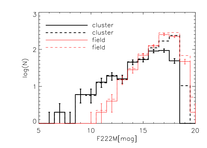
Figure 7.— Luminosity functions. Top panel: Observed LFs of stars detected in the F160W mosaics. The thick continuous line shows the GLIMPSE9 cluster LF after field subtraction, while the thick dashed line shows the same LF after correcting for incompleteness. Similarly, the thin lines show the LFs of the control field without (continuum) and with (dashed) correction for incompleteness. Middle panel: Observed LFs of stars detected in the F222M mosaics. Lower panel: LFs with the extinction free magnitude $\rm m_{e}$ of stars detected in both bands. Since $\rm m_{e}$ depends on color, we do not apply any extinction correction. Notice that Glimpse 9 has more luminous (massive) members.

3.4. Mass function

Apparent magnitudes of cluster members can be transformed into initial masses by assuming an interstellar extinction, a distance, and using an isochrone. We considered A${}_{\rm K_{\rm s}}$ $=1.6\pm 0.2$ mag, as estimated from the CMD (see above), and a distance of 4.2 kpc (Leahy et al., 2008). In addition, we used non-rotational models from the Geneva group, with increased mass-loss, Solar abundance, ages of 15, 20, and 27 Myr (Meynet et al., 1994), and with the color transformation for Johnson filters by Lejeune & Schaerer (2001). The relations between the actual mass and the apparent K-band magnitude for a 15, 20 and 27 Myr populations are shown in Fig. 8. We used the equations by Kim et al. (2005) to transform the theoretical isochrones for the F160W, F222M, and K_S short filters. An average difference of $0.07\pm 0.05$ mag is found between the K_S magnitudes from Kim et al. (2005) and those with the empirical transformation given in Sect. 2.2. This is a measure of the transformation uncertainty. Mass functions for the GLIMPSE9 cluster for different ages and bands are shown in Figs. 9 and 10.

We built mass functions for stars detected in the F160W mosaic, as well as for stars in the F222M mosaic. We selected a mass range log(M/M_⊙) from 0.1 to 0.8-0.9 to ensure that stars were above a completeness limit of 80% (see the Appendix), and to include only main-sequence stars (see Fig. 8). Evolved stars fall in a single bin because of the degenerate mass-luminosity relation (Fig. 8). For an age of 15 Myr, a linear fit to the mass function in the mass range from log(M/M_⊙) = 0.1 to 0.85 with a bin size of log(M/M_⊙)=0.05 yielded a slope of $-0.77\pm 0.20$ when using the F160W magnitudes, and of $-0.70\pm 0.25$ when using the F222M magnitudes. For an age of 20 Myr, the average slope from the two bands is $-0.63\pm 0.05$, while for an age of 27 Myr is $-0.64\pm 0.09$. Bin size variations from log(M/M_⊙)= 0.035 to 0.07 yield slopes with a standard deviation within 0.1, i.e. the uncertainty due to bin size variation is smaller than the uncertainty of the fit.

Besides this uncertainty due to age, the error in subtracting the foreground and background population needs also to be considered. If the control field is not representative of the background and foreground population seen towards the cluster, a systematic error is introduced when subtracting the field stars. The incorrect field subtraction would propagate into the LF and mass distribution. As seen in Fig. 1, the control field happens to be located in a dustier region. From the CMDs, the field appears to have an excess of red stars ($2<H-$K_S$<2.4$ mag), which implies an extra extinction of A${}_{\rm K_{\rm s}}$=$\sim 0.5$ mag. When artificially reducing the attenuation of the control field by A_K$=-0.5$ mag, the slope of the initial mass function decreases by $\sim 0.33$ ($-1.1\pm 0.1$, $-1.0\pm 0.16$, $-1.0\pm 0.1$ for 15, 20, and 27 Myr). We also calculated a mass function with the extinction free magnitudes $m_{e}$, which takes into account differential extinction, and measured a slope of $-1.0\pm 0.3$, $-0.96\pm 0.24$, and $-0.92\pm 0.27$ for 15, 20, and 27 Myr.

The origin and universality of the initial mass function remain under very active investigation and discussion. Typically, it is assumed as a power law with an exponent of $\Gamma=-1.35$ (Salpeter, 1955). Studies of starburst clusters, such as the Arches cluster, report flatter functions (e.g. $-0.7\pm 0.1$  Figer et al., 1999). Recent re-determinations of the Arches MF slope by Espinoza et al. (2009) indicate a slope of $-1.1\pm 0.2$, which is closer to a Salpeter.

The GLIMPSE9 cluster shows a mass function slightly flatter than the Salpeter’s one. We tried several ways to measure the mass function, including harshly de-reddening the control field, and yet we consistently come up with slopes that are shallower than Salpeter. Mass segregation, which bring massive stars to sink into the cluster center and low mass stars to disperse into the field, seems a plausible explanation for this (Kim et al., 2006). However, considered the uncertainties in age and background subtraction, and the fact that the GLIMPSE9 cluster is several million years old, a Salpeter initial mass function cannot be excluded.

Figure 8.— Actual mass versus apparent [F222M], for populations of 15, 20, and 27 Myr, with Solar abundance and increased mass-loss (Lejeune & Schaerer, 2001). A distance of 4.2 kpc, and A_K=1.6 mag are used.

Figure 9.— Background-subtracted mass functions of the GLIMPSE9 cluster from [F222M] or [F160W] magnitudes, for ages of 15, 20 and 27 Myr, are shown with a continuous line. The same function after correction for incompleteness is shown with a dashed line. Error bars represent the statistical Poisson uncertainty. Linear fits to bins with log(M/M_⊙) from 0.1 to 0.85-0.90 (i.e., F222M between 17.5 and 6.0 mag) are also shown.

Figure 10.— Background-subtracted mass functions of the GLIMPSE9 cluster from the extinction corrected $m_{e}$ magnitudes. Symbols as in Fig. 9

.

3.5. Cluster mass

By integrating the masses of the candidate member stars (using our background-subtracted mass function) down to a mass of 1.0 M_⊙, we measured a cluster mass of $1500\pm 300$ M_⊙, where the error takes into account the age uncertainty. Since systematic errors could be due to errors in the field subtraction, we also estimate the cluster mass by integrating only to K_S= 15 mag, i.e., by using the upper part of the diagram where field contamination is negligible, and extrapolating to 1.0 M_⊙ with a power law. When using the slope we estimated from the mass distribution, a mass of $1600\pm 400$ M_⊙ is obtained, while with the Salpeter mass distribution the mass value rises to $2100\pm 200$ M_⊙.

4. Cluster surroundings

4.1. A giant molecular cloud with SNRs

Table 2 Positions of the supernovae from literature.

ID	NAME	RA(J2000)	DEC(J2000)	velocity(km s-1)	diameter(′)	References
1	SNR/W41	18 34 46.42	$-$08 44 00	77$\pm$5	30.0	Green (1991); Leahy et al. (2008)
2	SNR22.7-0.2	18 33 17.86	$-$09 10 35	$\cdots$	30.0	Green (1991)
	G022.8$-$0.3	18 33 45.50	$-$09 09 17	82.5	10.9	Kuchar & Clark (1997)
3	$G22.7583-0.4917$	18 34 28.30	$-$09 16 00	74.8	4.7	Kuchar & Clark (1997)
		18 34 28.00	$-$09 16 00	76.0		Bronfman et al. (1996)
		18 34 26.70	$-$09 15 50	$\cdots$	5.0	#33 in Helfand et al. (2006)
4	$G22.9917-0.3583$	18 34 26.59	$-$09 00 09	$\cdots$	4.5	#34 in Helfand et al. (2006)
	$G22.9-0.3$	18 34 12.60	$-$09 01 20	70.9	4.8	Kuchar & Clark (1997)
5	$G23.5667-0.0333$	18 34 17.09	$-$08 20 21	$\cdots$	9.0	#35 in Helfand et al. (2006)
	$G23.5-0.0$	18 34 19.60	$-$08 22 17	91.3	6.1	Kuchar & Clark (1997)

Note. — Positions and dimensions were measured on the MAGPIS image.

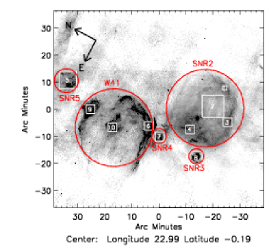
Figure 11.— 90 cm images from the Multi-Array Galactic Plane Imaging Survey (MAGPIS) (White et al., 2005). Grey circles show the locations of the SNRs listed in Table 2. White squares show the position of regions listed in Table 3, for which we calculated a spectral index. Longitude is along the x-axis, while latitude is along the y-axis.

The GLIMPSE9 cluster is located at (l,b)=(22.76 ^∘, -0.40 ^∘), in the direction of a GMC (Dame et al., 2001). The CO emission from the molecular cloud peaks near l=23.3 ^∘, b=-0.3 ^∘; it extends over two degrees in longitude with a line-of-sight velocity from 70 to 85 km s^-1 (Dame et al., 2001). Albert et al. (2006) derived an upper limit for the total H₂ mass of 2.1 $\times 10^{6}$ M_⊙, assuming a (near) kinematic distance of 4.9 kpc. The linear size of about 100 pc is in the range of other known giant molecular clouds. Several SNRs coincide in projection with this molecular cloud (see Fig. 11). Two SNRs are listed in the catalog of Green (1991), G022.7$-$00.2 and G023.8$-$00.3 (W41). Three other candidate SNRs were identified by Helfand et al. (2006), G$22.7583-0.4917$, G$22.9917-0.3583$, and G$23.5667-0.0333$. Leahy et al. (2008) concluded that the SNR W41 is associated with the GMC, and has a radial velocity $v_{LSR}$ = 77.0 km s^-1. Kuchar & Clark (1997) report $v_{LSR}$ = 82.5 km s^-1 for G022.8$-$00.3, and $v_{LSR}$ = 91.3 km s^-1 for G23.5$-$0.0. Bronfman et al. (1996) measured a $v_{LSR}$ = 76.0 km s^-1  towards G22.7583$-$0.4917. This suggests that at least three candidate SNRs are associated with the same GMC. In Table 2 we report positions of the candidate SNRs and associated line-of-sight velocity, when available. CO observations confirm a molecular cloud with a peak at $V_{LSR}=76\pm 5$ km s^-1 and a full-width-half-maximum of 22 km s^-1 at the location of the GLIMPSE9 cluster (Dame et al., 2001).

The classification of G022.7$-$00.2 is reported as uncertain by Green (1991), and the same radio source is listed as an HII region in other works (e.g. Kuchar & Clark, 1997; Paladini et al., 2003). We used archival radio data at 20 and 90 cm from the MAGPIS (White et al., 2005) to measure the radio spectral index of the candidate SNRs (see Fig. 11 and Table 3). Given the negative spectral indexes, the radio emission appears dominated by synchrotron emission in all cases. Since G$22.9917-0.3583$ and part of the radio shell of G022.7$-$00.2 overlaps with GLIMPSE 8 $\mu$m  emission, they are probably a composition of SNRs and HII regions. Assuming pure circular motion, a peak velocity of 78 km s^-1, a distance of 7.6 kpc for the Galactic Center, and a Solar V=214 km s^-1, a systematic deviation of 5 km s^-1, as well as a random deviation of 5 km s^-1, Leahy et al. (2008) derived a distance d=3.9-4.5 kpc for SNR/W41. Using an average distance of 4.2 kpc, the angular sizes of G022.7$-$00.2 and G023.3$-$00.3 (W41) ( $\sim$27^′) yield a linear size of $\sim$33 pc, while the angular sizes of G$22.7583-0.4917$, G$22.9917-0.3583$ and G$23.5667-0.0333$ (about 5 ^′) yield a linear size of $\sim$6pc. These physical sizes are well within the range of other Galactic SNRs (Stupar et al., 2007). Recently, Brunthaler et al. (2009) measured trigonometric parallaxes of 4.6 and 5.9 kpc with two methanol maser sources found towards G23.01$-$0.41 and G23.44$-$0.18, suggesting different complexes arranged along the line of sight.

Table 3 Spectral index from 90 and 20 cm MAGPIS data.

Region	RA(J2000)	DEC(J2000)	diameter(′′)	Spectral index
1	18:32:37.114	$-$09:13:32.15	77	$-$0.82
2	18:33:09.794	$-$09:12:45.87	384	$-$1.23
3	18:33:20.950	$-$09:20:17.81	154	$-$0.98
4	18:33:56.335	$-$09:09:13.63	154	$-$0.78
5	18:34:15.082	$-$08:20:41.93	307	$-$0.35
6	18:34:20.244	$-$08:55:07.61	154	$-$1.44
7	18:34:26.988	$-$09:00:23.31	154	$-$0.36
8	18:34:29.686	$-$09:16:03.12	230	$-$0.21
9	18:34:38.220	$-$08:33:10.46	154	$-$0.72
10	18:34:47.170	$-$08:43:24.00	154	$-$1.18

4.2. Stellar candidate clusters.

The presence of three SNRs with similar velocities ($v_{LSR}$ =75-85 km s^-1) suggests that massive star formation resulting in the production of several massive O stars has been active in multiple sites of this GMC. The stellar cluster GLIMPSE9 represents one episode of this star formation. Two other candidate clusters are reported in literature in the direction of the same molecular cloud. The $[BDS2003]$117 cluster (Bica et al., 2003) appears to be located onto the SNR shell G22.7583$-$0.4917, and the GLIMPSE10 cluster (the candidate number 10 in the list by Mercer et al., 2005) onto the SNR/W41 (see Fig. 12).

We searched for other stellar over-densities in the direction of this GMC. Detection of stellar over-densities are difficult due to the patchiness of the interstellar extinction. With the exception of GLIMPSE9 cluster, no clear over-densities were detected in the 2MASS images. To overcome interstellar extinction, we built a density map of point sources detected at 3.6 $\mu$m, which resulted in many spurious clumps. When looking at the SPITZER/GLIMPSE images, however, several nebular emissions are seen in all four IRAC channels of the SPITZER/GLIMPSE survey, indicating the presence of HII regions. An increased number of bright 3.6$\mu$m stars also appears associated with some of these regions. We therefore visually selected regions of nebular emission in all four IRAC channels or apparent over-densities of bright stars at 3.6$\mu$m. A list of the selected regions is given in Table 4.

We show 2MASS CMDs of these selected regions, together with a comparison CMD of the GLIMPSE9 cluster, in Fig. 13.

Several stellar branches are seen in each CMD, and each branch appears broadened by differential reddening. A bluer sequence with $H$-K_S$=\sim 0.4$ mag is visible in all CMDs. A redder sequence with $H$-K_S$=\sim 1$ mag, i.e., similar to that of the GLIMPSE9 cluster, appears only at certain locations. Assuming a distance of 4.2 kpc for the GMC, and considering an average of 1.8 mag of visual extinction per kpc, and the extinction law by Messineo et al. (2005), a stellar population associated with the GMC must have a minimum interstellar extinction of A${}_{\rm K_{\rm s}}$=0.7 mag. The bluer branch is probably due to a young stellar population associated with a closer spiral arm. Based on the similarity of interstellar extinction, we suggest that branches seen at $H$-K_S$=\sim 1$ mag are due to a stellar population associated with the GMC, similar to the GLIMPSE9 cluster.

Region 1, in the direction of SNR G$23.5-0.0$, shows nebular emission, but its 2MASS CMD does not show a stellar sequence with similar color as that of GLIMPSE9.

Region 2, in the direction of the SNR/W41, shows a peak of nebular emission in all four IRAC channels, indicating an HII region. The 2MASS diagrams also show a branch of bright stars at $H$-K_S$=\sim 0.8$ mag.

Region 3 shows a concentration of bright stars; however, no clear sequences are seen in the CMD.

Region 4 is also in the direction of SNR/W41. This region includes the GLIMPSE10 cluster, for which Mercer et al. (2005) gives a radius of 0.8^′; GLIMPSE10 coincides with a nebular peak emission, but the actual extension of the emission region has a radius of about 5^′. Several bright stars are detected in this region, and the 2MASS CMD shows a sequence at $H$-K_S$=\sim 1.0$ mag.

Region 5 coincides with the area covered by the SNR G22.9917$-$0.3583, as seen in the 90 cm image. A sequence at $H$-K_S$=\sim 1.0$ mag is detected.

Region 6 is a peak of a nebular emission that extends and connects to region 5. The CMD lacks stars in the redder sequence.

Region 7 coincides with the SNR G22.7583-0.4917. This region includes the $[BDS2003]$117 cluster area by Bica et al. (2003).

Two other regions, region 8 and region 9, were randomly selected, as a comparison fields. Region 8 does not show associated nebular emission, and is in the direction of the SNR/W41. The CMD shows the blue sequence, but not a clear red sequence. Region 9, which is at the outer edge of the complex, does not show nebular emission, and its CMD lacks a sequence at $H$-K_S$=\sim 1.0$ mag.

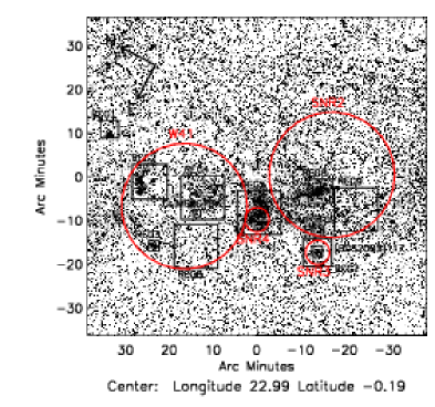
Figure 12.— The greyscale shows a 3.6 $\mu$m GLIMPSE image. Circles show the locations of the four SNRs. Squares and labels show the regions in Table 4. Longitude is along the x-axis, while latitude is along the y-axis.

Table 4 Cluster positions.

ID	RA(J2000)	DEC(J2000)	Radius(′)	References
GLIMPSE9	18 34 09.59	$-$09 13 53	0.3	Mercer et al. (2005)
$[BDS2003]$117	18 34 27.00	$-$09 15 42	0.6	Bica et al. (2003)
GLIMPSE10	18 34 47.00	$-$08 47 20	0.8	Mercer et al. (2005)
Region1	18 34 15.08	$-$08 20 42	1.2
Region2	18 34 41.09	$-$08 34 22	4.0
Region3	18 35 32.22	$-$08 41 56	1.2
Region4	18 34 31.59	$-$08 46 47	5.0
Region5	18 34 20.00	$-$08 59 48	5.0
Region6	18 33 36.03	$-$09 10 01	2.7
Region7	18 34 27.69	$-$09 15 52	3.3
Region8	18 35 14.46	$-$08 50 34	5.0
Region9	18 33 35.88	$-$09 19 08	5.0

Note. — Coordinates are followed by radius and references. Region #8 and #9 are randomly selected.

Figure 13.— 2MASS J$-$K_S versus K_S, and H$-$K_S versus K_S diagrams of selected regions in direction of the GMC (see Table 4). For clarity, an area of 3^′ is used for all CMDs. Two vertical lines at ($H-$K_S$=0.6$ and 1.4 mag indicate the color region of the GLIMPSE9 sequence. A similar sequence is visible in reg #2,#4, #5 and #7.

Figure 13.— 13 continued.

5. Summary

Investigation with HST/NICMOS data confirms that object number 9 in the list by Mercer et al. (2005) is a stellar cluster with a well defined sequence in the $H-$K_S  versus K_S diagram. Low-resolution spectroscopic observations in K-band yield the spectral types of the brightest candidate members, and confirm the presence of massive stars. Three RSGs are detected, two of which are candidate cluster members, and two BSGs. A spectrophotometric distance of $4.2\pm 0.4$ kpc is derived, an age between 15 and 27 Myr, and a mass of at least $1600\pm 400$ M_⊙. The cluster mass function appears slightly flatter than the Salpeter’s one, which could be the effect of mass segregation.

The cluster is located in the direction of a molecular complex, which hosts several SNRs and HII regions. The cluster distance agrees well with that inferred for the complex by Leahy et al. (2008). A stellar population possibly associated with the giant molecular cloud is seen in four other regions: two regions are associated with the SNR/W41, one region with the SNR G22.9917$-$0.3583, and another region with SNR G22.7583-0.4917. The detection of massive stars in GLIMPSE9, and the concomitant presence of several SNRs render this GMC particular interesting. It is a good laboratory to investigate various issues about massive stars and multi-seeded star formation. By identifying stellar clusters of the same complex, one can study their properties and variations across space and time. Some of the most massive stars of the Milky Way may be hiding among the cluster members. The detection of short lived massive stars (e.g. Wolf-Rayets, Red Supergiants, Luminous Blue Variables) is important to understand their formation, evolution and fate. By association with the SNRs, massive stars also yield the initial masses of the supernova progenitors. A more detailed study of this complex will be presented in a future paper.

Appendix A Artificial-star experiments

For a proper cluster analysis (e.g. for a statistical field decontamination, luminosity function, and mass function studies), one needs to characterize all undesired biases of photometric measurements in dense stellar fields. Crowding limits the detection of point sources, and such incompleteness varies from field to field because it depends on the stellar density. We, therefore, run simulations with artificial stars.

Artificial stars were created with the observed PSF. Then, the artificial stars were added into each mosaic at random positions, but imposing only one star over a $50\times 50$ pixels area in order not to alter the level of crowding. The luminosity function of the artificial stars was assumed identical to the observed luminosity function of each frame. The photometry of the artificial stars was recovered following the exact steps as those performed for the actual catalog. The procedure was iterated 300 times, giving a total of 27,000 artificial stars per mosaic. By comparing the fluxes of the artificial stars’ input with their fluxes after re-extraction, we obtained an estimate of the photometric uncertainty and completeness limit.

In Figure 14 the differences between the input ($mag_{input}$) and the extracted magnitudes ($mag_{output}$) of the artificial stars are shown as a function of $mag_{input}$; differences remain, on average, null till a certain magnitude, then increase with increasing $mag_{input}$; this is due to blending between artificial stars and real stars, and it causes a bin-to-bin migration in the luminosity function (LF). A star is considered lost if no star is located by the DAOPHOT point-source finding algorithm within 1.5 pixels (0.1^′′) of the inserted location. The fraction of recovered stars per bin of magnitude is the completeness factor (C_f). A C_f above 80% is reached for $[F222M]<17.0$ mag in the cluster field, and $[F222M]<18.0$ mag in the control field. For the cluster field, the one sigma deviation is below 0.3 mag for $[F222M]<\sim 16.0$ mag, but 1.0 mag for $[F222M]=\sim 18.5$ mag. In the control field, the one sigma deviation is below 0.3 mag for $[F222M]<18$ mag, and 1.0 mag for $[F222M]=\sim 20$ mag.

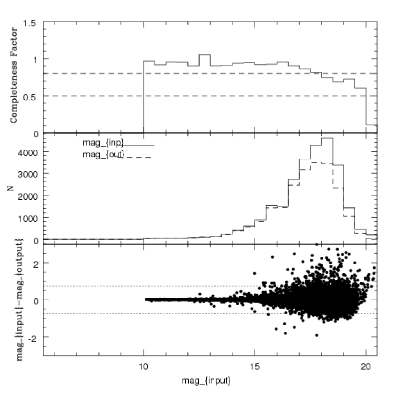
Figure 14.— Completeness experiment for the cluster field observation with the F222M filter. Cluster data are shown in the top figure, and field data are shown in the figure at the bottom. Lower-panel: The differences between input and output magnitudes are shown ($mag_{input}-mag_{output}$). The dashed lines indicate a difference of $\pm 0.75$ mag. Middle panel shows the distribution in magnitudes of the artificial stars (a solid line is used for the input magnitudes, a dashed line for the output magnitudes). Upper panel: The ratio between the number of stars in output and in input is shown, as a function of magnitude. Two dotted lines indicated the 80% and 50% completeness limits.

References

- Albert et al. (2006) Albert, J., Aliu, E., Anderhub, H., et al. 2006, ApJ, 648, L105
- Alvarez et al. (2000) Alvarez, R., Lançon, A., Plez, B., & Wood, P. R. 2000, A&A, 353, 322
- Bibby et al. (2008) Bibby, J. L., Crowther, P. A., Furness, J. P., & Clark, J. S. 2008, MNRAS, 386, L23
- Bica et al. (2003) Bica, E., Dutra, C. M., Soares, J., & Barbuy, B. 2003, A&A, 404, 223
- Blum et al. (2000) Blum, R. D., Conti, P. S., & Damineli, A. 2000, AJ, 119, 1860
- Blum et al. (2003) Blum, R. D., Ramírez, S. V., Sellgren, K., & Olsen, K. 2003, ApJ, 597, 323
- Blum et al. (1996) Blum, R. D., Sellgren, K., & Depoy, D. L. 1996, AJ, 112, 1988
- Bronfman et al. (1996) Bronfman, L., Nyman, L.-A., & May, J. 1996, A&AS, 115, 81
- Brunthaler et al. (2009) Brunthaler, A., Reid, M. J., Menten, K. M., et al. 2009, ApJ, 693, 424
- Clark et al. (2009a) Clark, J. S., Davies, B., Najarro, F., & Mackenty, J. 2009a, A&A, 504, 429
- Clark et al. (2009b) Clark, J. S., Negueruela, I., Davies, B., et al. 2009b, A&A, 498, 109
- Dame et al. (2001) Dame, T. M., Hartmann, D., & Thaddeus, P. 2001, ApJ, 547, 792
- Davies et al. (2007) Davies, B., Figer, D. F., Kudritzki, R.-P., et al. 2007, ApJ, 671, 781
- Espinoza et al. (2009) Espinoza, P., Selman, F. J., & Melnick, J. 2009, A&A, 501, 563
- Figer et al. (1999) Figer, D. F., Kim, S. S., Morris, M., et al. 1999, ApJ, 525, 750
- Figer et al. (2006) Figer, D. F., MacKenty, J. W., Robberto, M., et al. 2006, ApJ, 643, 1166
- Froebrich et al. (2007) Froebrich, D., Scholz, A., & Raftery, C. L. 2007, MNRAS, 374, 399
- Giveon et al. (2005) Giveon, U., Becker, R. H., Helfand, D. J., & White, R. L. 2005, AJ, 130, 156
- Green (1991) Green, D. A. 1991, PASP, 103, 209
- Hanson et al. (1996) Hanson, M. M., Conti, P. S., & Rieke, M. J. 1996, ApJS, 107, 281
- Hanson et al. (2005) Hanson, M. M., Kudritzki, R.-P., Kenworthy, M. A., Puls, J., & Tokunaga, A. T. 2005, ApJS, 161, 154
- Helfand et al. (2006) Helfand, D. J., Becker, R. H., White, R. L., Fallon, A., & Tuttle, S. 2006, AJ, 131, 2525
- Homeier & Alves (2005) Homeier, N. L. & Alves, J. 2005, A&A, 430, 481
- Ivanov et al. (2004) Ivanov, V. D., Rieke, M. J., Engelbracht, C. W., et al. 2004, ApJS, 151, 387
- Kim et al. (2006) Kim, S. S., Figer, D. F., Kudritzki, R. P., & Najarro, F. 2006, ApJ, 653, L113
- Kim et al. (2005) Kim, S. S., Figer, D. F., Lee, M. G., & Oh, S. 2005, PASP, 117, 445
- Kleinmann & Hall (1986) Kleinmann, S. G. & Hall, D. N. B. 1986, ApJS, 62, 501
- Koornneef (1983) Koornneef, J. 1983, A&A, 128, 84
- Kuchar & Clark (1997) Kuchar, T. A. & Clark, F. O. 1997, ApJ, 488, 224
- Kumar et al. (2004) Kumar, N. M. S., Kamath, U. S., & Davis, C. J. 2004, MNRAS, 353, 1025
- Lada & Lada (2003) Lada, C. J. & Lada, E. A. 2003, ARA&A, 41, 57
- Leahy et al. (2008) Leahy, D. A. & Tian, W. 2008, AJ, 135, 167
- Lejeune & Schaerer (2001) Lejeune, T. & Schaerer, D. 2001, A&A, 366, 538
- Levesque et al. (2005) Levesque, E. M., Massey, P., Olsen, K. A. G., et al. 2005, ApJ, 628, 973
- MacKenty et al. (2003) MacKenty, J. W., Greenhouse, M. A., Green, R. F., et al. 2003, in Presented at the Society of Photo-Optical Instrumentation Engineers (SPIE) Conference, Vol. 4841, Society of Photo-Optical Instrumentation Engineers (SPIE) Conference Series, ed. M. Iye & A. F. M. Moorwood, 953–961
- Mercer et al. (2005) Mercer, E. P., Clemens, D. P., Meade, M. R., et al. 2005, ApJ, 635, 560
- Messineo et al. (2009) Messineo, M., Davies, B., Ivanov, V. D., et al. 2009, ApJ, 697, 701
- Messineo et al. (2008) Messineo, M., Figer, D. F., Davies, B., et al. 2008, ApJ, 683, L155
- Messineo et al. (2005) Messineo, M., Habing, H. J., Menten, K. M., et al. 2005, A&A, 435, 575
- Meynet & Maeder (2003) Meynet, G. & Maeder, A. 2003, A&A, 404, 975
- Meynet et al. (1994) Meynet, G., Maeder, A., Schaller, G., Schaerer, D., & Charbonnel, C. 1994, A&AS, 103, 97
- Oliva & Origlia (1992) Oliva, E. & Origlia, L. 1992, A&A, 254, 466
- Paladini et al. (2003) Paladini, R., Burigana, C., Davies, R. D., et al. 2003, A&A, 397, 213
- Salpeter (1955) Salpeter, E. E. 1955, ApJ, 121, 161
- Siess et al. (2000) Siess, L., Dufour, E., & Forestini, M. 2000, A&A, 358, 593
- Skrutskie et al. (2006) Skrutskie, M. F., Cutri, R. M., Stiening, R., et al. 2006, AJ, 131, 1163
- Smith et al. (2009) Smith, R. J., Clark, P. C., & Bonnell, I. A. 2009, MNRAS, 396, 830
- Stetson (1987) Stetson, P. B. 1987, PASP, 99, 191
- Stupar et al. (2007) Stupar, M., Filipović, M. D., Parker, Q. A., et al. 2007, Ap&SS, 307, 423
- Subramaniam et al. (2006) Subramaniam, A., Mathew, B., Bhatt, B. C., & Ramya, S. 2006, MNRAS, 370, 743
- Tsuji (2000) Tsuji, T. 2000, ApJ, 538, 801
- Wallace & Hinkle (1996) Wallace, L. & Hinkle, K. 1996, ApJS, 107, 312
- White et al. (2005) White, R. L., Becker, R. H., & Helfand, D. J. 2005, AJ, 130, 586