Quantum phase transitions of the extended  isotropic XY model with long-range interactions

Abstract

The one-dimensional extended isotropic XY model (s=1/2) in a transverse field with uniform long-range interactions among the z components of the spin is considered. The model is exactly solved by introducing the gaussian and Jordan-Wigner transformations, which map it in a non-interacting fermion system. The partition function can be determined in closed form at arbitrary temperature and for arbitrary multiplicity of the multiple spin interaction. From this result all relevant thermodynamic functions are obtained and, due to the long-range interactions, the model can present classical and quantum transitions of first- and second-order. The study of its critical behavior is restricted for the quantum transitions, which are induced by the transverse field at $T=0.$ The phase diagram is explicitly obtained for multiplicities $p=2,3,4$ and $\infty,$ as a function of the interaction parameters, and, in these cases, the critical behavior of the model is studied in detail. Explicit results are also presented for the induced magnetization and isothermal susceptibility $\chi_{T}^{zz}$, and a detailed analysis is also carried out for the static longitudinal $\langle S_{j}^{z}S_{l}^{z}\rangle$ and transversal $\langle S_{j}^{x}S_{l}^{x}\rangle$ correlation functions. The different phases presented by the model can be characterized by the spatial decay of the these correlations, and from these results some of these can be classified as quantum spin liquid phases. The static critical exponents and the dynamic one, $z,$ have also been determined, and it is shown that, besides inducing first order phase transition, the long-range interaction also changes the universality class the model.

identifier

I Introduction

The study of the quantum phase transitions(QPTs) has been the object of many theoretical and experimental investigationsSchadev 2000 , since they play an essential role in understanding the low temperature properties of the materialsColeman 2005 . In particular, for low dimension magnetic materials, the study of quantum spin chains has provided much insight in this directionSchadev 2008 . Motivated by this, in the last years, others tools have been used to investigate QPTs in spin chains, such as, quantum discordRaoul 2008 , geometric phasesCarollo 2005 ; Zhu 2006 and quantum fidelityZanardi 2006 , where the last two concepts were unified in the approach of the geometric tensorsVenuti 2007 . All these tools have only one purpose, that is, to point out the existence of the quantum critical behavior. On the other hand, the QPTs are also directly related to quantum entanglement, which has been object of study in quantum computationAmico 2006 . Therefore, the study of spin systems is of great importance for understanding the behavior of the materials in low temperature regime.

Among the quantum spin models, the one-dimensional XY model introduced by Lieb et al.Lieb 1961 , with its generalized classes, have attracted much interest in the last decades. In particular, the models with multiple spin (see Refs.Titvinidze 2003 ; Krokhmalskii2008 , and references therein) and long-range interactions(see Refs. Lenilson 2005 ; Bouchett 2008 , and references therein) have been object of intensive investigations. As pointed out by DerzhkoDerzhko 2009 and in the references therein, quantum spin systems with multiple spin interactions work as effective spin models for the standard Hubbard model under certain conditions. On the other hand, models with long-range interactions are important to understand the process of quantum information in spin chains as well as for the study of the classical and/or quantum crossover, as it was explained by de Lima and Gonçalves.de Lima 2008 . Another importance of the long-range interaction is that it can induce first-order QPTs, which play an important role in the quantum critical behaviourPfleiderer 2005 .

Therefore, in this paper, we will study the effect of the long-range interaction on the quantum critical behaviour of the extended one-dimensional XY-model with multiple spin interactionsSuzuki 1971 . The solution of the model can be obtained exactly, at arbitrary temperatures in a one-dimensional and the main purpose of the paper is to study the quantum critical behaviour of the model.

We analyze these two kind of interactions, where we will show the role of each one, that is, we will show that the long-range interactions induce first and second order QPTs and that their presence change the universality class of the model, as we will also verify the scaling relations proposed by Continentino and FerreiraContinentino 2004 for first-order QPTs. While for the multisite interaction among spins, we will show the presence of many different kinds of quantum spin liquid phases, which after some time returned to be a relevant topic in the present researchLee 2008 .

In Sec. II we introduce the model and obtain its exact solution by means of  Jordan-Wigner fermionization and the integral  Gaussian transformation, and present its basic results, such as, the spectrum of the energy, magnetization at arbitrary temperatures. The quantum phase diagrams, as function of the interaction parameters, are presented and discussed in Sec. III, and in Sec. IV we study the scaling behaviour of the longitudinal and transversal correlations functions on the different phases presented by the model. In Sec. V we evaluate the critical exponents, and discuss the change in the universality class due the presence of the long-range interactions. Finally, in Sec. VI we summarize the main results.

II THE MODEL AND BASIC RESULTS

We consider the one-dimensional isotropic extended XY model ($s=1/2$) with uniform long-range interactions among the $z$ components of the spins,  whose Hamiltonian is explicitly given by

$$\mathcal{H} =-J_{1}\sum_{j=1}^{N}(S_{j}^{x}S_{j+1}^{x}+S_{j}^{y}S_{j+1}^{y})-\frac{I}{N}\sum_{j=1}^{N}\sum_{l=1}^{N}S_{j}^{z}S_{l}^{z}-h\sum_{j=1}^{N}S_{j}^{z}-$$

$$-J_{2}\sum_{j=1}^{N}\sum_{\kappa=2}^{p}(S_{j}^{x}S_{j+\kappa}^{x}+S_{j}^{y}S_{j+\kappa}^{y})S_{j+1}^{z}S_{j+2}^{z}...S_{j+\kappa-1}^{z},$$ (1)

where the parameters $J_{1}$, $J_{2}$ are the exchange coupling between nearest neighbors, $I$ the uniform long-range interaction among the $z$ components, $p$ is the multiplicity of the multiple spin interaction, and $N$ is the number of sites of the lattice.

Introducting the Jordan-Wigner transformation

$$S_{j}^{+}=\left[\text{exp}\left(i\pi\sum_{l=1}^{j-1}c_{l}^{\dagger}c_{l}\right)\right]c_{j}^{\dagger}\hskip 2.84544pt;\hskip 14.22636ptS_{j}^{-}=c_{j}\left[\text{exp}\left(-i\pi\sum_{l=1}^{j-1}c_{l}^{\dagger}c_{l}\right)\right],$$ (2)

$$S_{j}^{z}=c_{j}^{\dagger}c_{j}-\frac{1}{2},$$ (3)

where $c_{j}$ and $c_{j}^{\dagger}$ are fermion operators, the Hamiltonian can be written in the well known decomposed form(siskens 1974 also references therein)

$$\mathcal{H}=\mathcal{H}^{+}P^{+}+\mathcal{H}^{-}P^{-},$$ (4)

where

$$\mathcal{H}^{\pm} =-\frac{J_{1}}{2}\sum_{j=1}^{N-1}\left(c_{j}^{\dagger}c_{j+1}+c_{j+1}^{\dagger}c_{j}\right)-\left(h-I\right)\sum_{j=1}^{N}c_{j}^{\dagger}c_{j}-\frac{I}{N}\sum_{j=1}^{N}\sum_{l=1}^{N}c_{j}^{\dagger}c_{j}c_{l}^{\dagger}c_{l}$$ (5)

$$-{}\frac{J_{2}}{2}\sum_{j=1}^{N-p}\sum_{k=2}^{p}\left(\frac{-1}{2}\right)^{k-1}\left(c_{j}^{\dagger}c_{j+k}+c_{j+k}^{\dagger}c_{j}\right)+\frac{N}{2}\left(h-\frac{I}{2}\right)$$

$$\pm\frac{J_{1}}{2}\left(c_{N}^{\dagger}c_{1}+c_{1}^{\dagger}c_{N}\right)\pm{}\frac{J_{2}}{2}\sum_{l=1}^{p}\sum_{\begin{subarray}{c}k=2\\ p-l\geq 2\end{subarray}}^{p-l}\left(\frac{-1}{2}\right)^{k-1}\left(c_{N-p+l}^{\dagger}c_{l-p+k}+c_{l-p+k}^{\dagger}c_{N-p+l}\right)\pm$$

$$\pm\frac{J_{2}}{2}\sum_{l=1}^{p}\sum_{\begin{subarray}{c}k=p-l+1\\ k\geq 2\end{subarray}}^{p}\left(\frac{-1}{2}\right)^{k-1}\left(c_{N-p+l}^{\dagger}c_{l-p+k}+c_{l-p+k}^{\dagger}c_{N-p+l}\right),$$

and

$$P^{\pm}=\frac{I\pm P}{2},$$ (6)

with $P$ given by

$$P=\exp\left(i\pi\sum_{l=1}^{N}c_{l}^{\dagger}c_{l}\right).$$ (7)

As it is also well known, the Hamiltonian $\mathcal{H}^{\pm}$ can be diagonalized by imposing  antiperiodic (for $\mathcal{H}^{+})$ and periodic (for $\mathcal{H}^{-})$ boundary conditions, and, in the thermodynamic limit, the static properties can be described by $\mathcal{H}^{-}$ siskens 1974 ; capel 1977 ; goncalves 1977 . Therefore, since we are interested in the determination of the static properties, we will identify the Hamiltonian of the system with $\mathcal{H}^{-}.$ By taking into account that the long-range interaction term commutes with the Hamiltonian, the partition can be written in the form

$$\mathcal{Z_{N}} =\text{exp}\left[-\frac{\beta N}{2}\left(h-\frac{I}{2}\right)\right]Tr\left\{\text{exp}\left[\frac{\beta J_{1}}{2}\sum_{j=1}^{N}\left(c_{j}^{\dagger}c_{j+1}+c_{j+1}^{\dagger}c_{j}\right)+\right.\right.{}$$

$${}\left.\left.+\beta\left(h-I\right)\sum_{j=1}^{N}c_{j}^{\dagger}c_{j}+\frac{\beta J_{2}}{2}\sum_{j=1}^{N}\sum_{\kappa=2}^{p}\left(\frac{-1}{2}\right)^{\kappa-1}\left(c_{j}^{\dagger}c_{j+\kappa}+c_{j+\kappa}^{\dagger}c_{j}\right)\right]\right.{}$$

$${}\left.\times\text{exp}\left[\frac{\beta I}{N}\sum_{j=1}^{N}\sum_{l=1}^{N}c_{j}^{\dagger}c_{j}c_{l}^{\dagger}c_{l}\right]\right\},$$ (8)

where $\beta=1/k_{B}T$ and $T$ is the temperature. Introducting the Gaussian transformationamit1984

$$\text{exp}(a^{2})=\frac{1}{\sqrt{2\pi}}\int_{-\infty}^{\infty}\text{exp}\left(-\frac{x^{2}}{2}+\sqrt{2}ax\right)dx,$$ (9)

the partition function can be written in the integral representation as

$$\mathcal{Z_{N}} =\text{exp}\left[-\frac{N}{2}\left(\overline{h}-\frac{\overline{I}}{2}\right)\right]\sqrt{\frac{N}{2\pi}}\int_{-\infty}^{\infty}\exp\left(-\frac{N\overline{x}^{2}}{2}\right)Tr\left\{\text{exp}\left[\frac{\overline{J}_{1}}{2}\sum_{j=1}^{N}\left(c_{j}^{\dagger}c_{j+1}+c_{j+1}^{\dagger}c_{j}\right)+\right.\right.{}$$

$${}\left.+\left(\overline{h}-\overline{I}+2\sqrt{\overline{I}}\overline{x}\right)\sum_{j=1}^{N}c_{j}^{\dagger}c_{j}+\frac{\overline{J}_{2}}{2}\sum_{j=1}^{N}\sum_{\kappa=2}^{p}\left(\frac{-1}{2}\right)^{\kappa-1}\left(c_{j}^{\dagger}c_{j+\kappa}+c_{j+\kappa}^{\dagger}c_{j}\right)\right]d\overline{x},$$ (10)

where $\overline{x}\equiv x/\sqrt{N},\overline{J}_{1}\equiv\beta J_{1},\overline{J}_{2}\equiv\beta J_{2},\overline{h}\equiv\beta h$ and $\overline{I}=\beta I.$

Introducing the canonical transformation

$$c_{j}=\frac{1}{\sqrt{N}}\sum_{q=1}^{N}\exp\left(ijq\right)c_{q}\ \ \ \ \ \text{and}\ \ \ \ \ \ \ c_{j}^{\dagger}=\frac{1}{\sqrt{N}}\sum_{q=1}^{N}\exp\left(-ijq\right)c_{q}^{\dagger},$$ (11)

with  $q=2\pi n/N,$ $n=1,2,...,N,$ Eq. (10)  can be written in the form

$${\mathcal{Z_{N}}=C(\beta)\int_{-\infty}^{\infty}\exp\left(-\frac{N\overline{x}^{2}}{2}\right)\zeta\left(\overline{x}\right)d\overline{x},}$$ (12)

where

$$C(\beta)=\sqrt{\frac{N}{2\pi}}\text{exp}\left[-\frac{N}{2}\left(\overline{h}-\frac{\overline{I}}{2}\right)\right],\ \ \ \ \ \ \ \ \ \ \ \ \zeta\left(\overline{x}\right)=Tr\left\{\exp\left[\sum_{q}\overline{\epsilon}_{q}\left(\overline{x}\right)c_{q}^{\dagger}c_{q}\right]\right\},$$ (13)

with

$$\overline{\epsilon}_{q}\left(\overline{x}\right)=\beta\left[J_{1}\cos(q)+J_{2}\sum_{\kappa=2}^{p}\left(-\frac{1}{2}\right)^{\kappa-1}\cos(\kappa q)+h-I+\sqrt{\frac{2I}{\beta}}\overline{x}\right].$$ (14)

In the thermodynamic limit, $N\rightarrow\infty$, we use the Laplace’s methodmurray 1984 to evaluate the partition function, and ${\mathcal{Z_{N}}}$ can be written in the form

$${\mathcal{Z_{N}=}}\frac{\exp\left[-\frac{N}{2}\left(\overline{h}-\frac{\overline{I}}{2}\right)+Ng(\overline{x}_{0})\right]}{\mid g^{\prime\prime}(\overline{x}_{0})\mid^{1/2}},$$ (15)

where

$$g(\overline{x}_{0})=-\frac{\overline{x}_{0}^{2}}{2}+\frac{1}{N}\sum_{q}\ln\left[1+\exp\left(\overline{\epsilon}_{q}\left(\overline{x}_{0}\right)\right)\right],$$ (16)

with $g(\overline{x}_{0})\$satisfying the conditions

$$g^{\prime}(\overline{x}_{0})=0,\text{ \ \ \ \ \ and\ \ \ \ \ \ \ }g^{\prime\prime}(\overline{x}_{0})<0,$$ (17)

and $\overline{x}_{0}$ explicitly given by

$$\overline{x}_{0}=\frac{\sqrt{2\overline{I}}}{N}\sum_{q=1}^{N}\frac{1}{1+\exp(-\overline{\epsilon}_{q}\left(\overline{x}_{0}\right))}.$$ (18)

Therefore, from Eq.(15) we can write the Helmholtz free energy as

$$F_{N}=\frac{N}{2}\left(h-\frac{I}{2}\right)-Nk_{B}Tg(\overline{x}_{0})+\frac{k_{B}T}{2}\ln\mid g^{\prime\prime}(\overline{x}_{0})\mid.$$ (19)

Taking into account that the magnetization per site $M^{z}$ can be written in the form

$$M^{z}=\frac{1}{N}\sum_{j}\langle S_{j}^{z}\rangle=\frac{1}{N}\sum_{q}\langle c_{q}^{\dagger}c_{q}\rangle-\frac{1}{2}=\frac{1}{N}\sum_{q}\frac{1}{1+\exp\left[-\overline{\epsilon}_{q}\left(\overline{x}\right)\right]}-\frac{1}{2},$$

by using Eq.(18), we can express $\overline{x}_{0}$ in terms of $M^{z}$ in the form

$$\overline{x}_{0}=\sqrt{2\overline{I}}\left(M^{z}+\frac{1}{2}\right),$$ (20)

and from this result it follows that the functional of the Helmholtz free energy per site is given by

$$f=\frac{h}{2}+IM^{z}\left(1+M^{z}\right)+\frac{k_{B}T}{\pi}\int_{0}^{\pi}\ln\left(1+\exp\left[\overline{\epsilon}_{q}\left(M^{z}\right)\right]\right)dq,$$ (21)

with

$$\overline{\epsilon}_{q}\left(M^{z}\right)=-\overline{J}_{1}\cos(q)-\overline{J}_{2}\sum_{\kappa=2}^{p}\left(-\frac{1}{2}\right)^{\kappa-1}\cos(\kappa q)-\overline{h}-2\overline{I}M^{z}.$$ (22)

From Eq. (21), we can  determine the equation of state  imposing  the stability conditions

$$\frac{\partial f}{\partial M^{z}} =0,\text{ \ \ \ \ \ }$$ (23)

$$\text{\ \ \ \ }\frac{\partial^{2}f}{\partial M^{z2}} >0,$$ (24)

which leads to the result

$$M^{z}=\frac{1}{2\pi}\int_{0}^{\pi}\tanh\left[\frac{\overline{\epsilon}_{q}\left(M^{z}\right)}{2}\right]dq.$$ (25)

III QUANTUM CRITICAL BEHAVIOR

In the limit $T\rightarrow 0$, the functional of the Helmholtz free energy per site[Eq. (21)] is given by

$$f=\frac{h}{2}+IM^{z}\left(1+M^{z}\right)-\frac{1}{\pi}{\displaystyle\int\limits_{\epsilon_{q}\left(M^{z}\right)<0}}\epsilon_{q}\left(M^{z}\right)dq,$$ (26)

where

$$\epsilon_{q}\left(M^{z}\right)=J_{1}\cos(q)+J_{2}\sum_{\kappa=2}^{p}\left(-\frac{1}{2}\right)^{\kappa-1}\cos(\kappa q)+h+2IM^{z},$$ (27)

and the equation of state, given by Eq. (25), can be written in the form

$$M^{z}=\frac{1}{2\pi}\int_{0}^{\pi}sign\left[\epsilon_{q}\left(M^{z}\right)\right]dq.$$ (28)

The quantum phase diagram of the model, for second order phase transitions and arbitrary $p$, can be obtained from the previous expression by imposing the divergence of the isothermal susceptibility, $\chi_{T}^{zz}\equiv\partial M^{z}/\partial h\rightarrow\infty,$ and for first-order phase transitions, by using the equation of state, Eq. (25), and by imposing the condition

$$f(M_{it}^{z})=f(M_{jt}^{z}),$$ (29)

where $M_{it}^{z}$ and $M_{jt}^{z}$ are the values of the induced magnetization at the transition.

Following Titvinidze and JaparidzeTitvinidze 2003 , by introducing the unitary transformation

$$S_{j}^{x,y}\rightarrow\left(-1\right)^{j}S_{j}^{x,y}\text{ \ \ \ \ ; \ }S_{j}^{z}=S_{j}^{z},$$ (30)

and the time reversal one

$$S_{j}^{x,z}\rightarrow-S_{j}^{x,z}\text{ \ \ \ \ ; \ }S_{j}^{y}=S_{j}^{y},$$ (31)

we can show that the Hamiltonian is invariant under the transformation $J_{1}\rightarrow-J_{1}$ and $J_{2}\rightarrow-J_{2}.$ This means that only the signs of $I$ and $J_{2}$ are relevant in determining the critical behaviour of the system, and the appearance of multiple phases are result of the competition between these interactions which induce frustration in the system. In particular, they can induce the so-called quantum spin liquid phasesLee 2008 , as in the case of the model without long-range interactionTitvinidze 2003 . Therefore, without loss of generality, we will consider in all results presented $J_{1}>0$ only.

From Eqs. (26-28), we can show that, for arbitrary $p,$ the system presents second order quantum transitions for $I\leq 0$, and first-order quantum transitions $I>0,$ as in the previously studied XY-models with similar long-range interactionsLenilson 2005 .

Although the Eqs. (26-28) allow us to obtain the phase diagrams for arbitrary $p$, we will only consider the cases $p=2,3,4$ and $\infty,$ since they present the main features and, in these cases, analytical expressions can be obtained for the critical surfaces and critical lines associated to the second order quantum transitions.

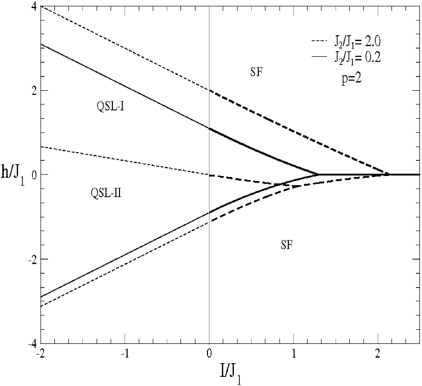
Figure 1: Phase diagram for the quantum transitions  as a function of the long-range interaction $I/J_{1}$ for $p=2$ and $J_{2}/J_{1}=0.2,2.0.$ For $J_{2}/J_{1}=0.2$ there are three phases, one spin liquid phase (QSL-I) and two saturated ferromagnetic phases(SF), and for $J_{2}/J_{1}=2.0,$ there are four phases, two spin liquid phases (QSL-I,QSL-II) and two saturated ferromagnetic phases(SF). The critical lines correspond to first-order phase transitions for $I/J_{1}>0$ and to second-order phase transitions for $I/J_{1}\leq 0.$

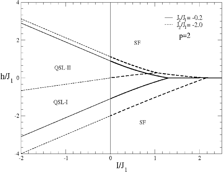
Figure 2: Phase diagram for the quantum transitions  as a function of the long-range interaction $I/J_{1}$ for $p=2$ and $J_{2}/J_{1}=-0.2,-2.0.$ For $J_{2}/J_{1}=-0.2$ there are three phases, one spin liquid phase (QSL-I) and two saturated ferromagnetic phases(SF), and for $J_{2}/J_{1}=-2.0,$ there are four phases, two spin liquid phases (QSL-I,QSL-II) and two saturated ferromagnetic phases(SF). The critical lines correspond to first-order phase transitions for $I/J_{1}>0$ and to second-order phase transitions for $I/J_{1}\leq 0.$

For the case $p=2,$ which has also been studied by Titvinidze and JaparadzeTitvinidze 2003 and Krokhmalski et al. Krokhmalskii2008 for the model without long-range interactions, we show in Figs. 1 and 2 the critical field $h/J_{1}$ as a function of $I/J_{1}$ in the regions $J_{2}/J_{1}\geq 0$ and $J_{2}/J_{1}\leq 0,$ respectively,  for different values $J_{2},$ which are projections of the global phase diagram. It is worth mentioning that in this case the results for $J_{2}/J_{1}\leq 0$ can be  obtained from the results for $J_{2}/J_{1}\geq 0$ by introducing the transformations $h/J_{1}\rightarrow-h/J_{1}$ and $J_{2}/J_{1}\rightarrow-J_{2}/J_{1},$ as can be verified in the results shown in Figs. 1 and 2.

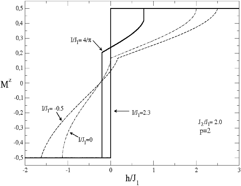
Figure 3: Magnetization $M^{z}$ as a function of $h/J_{1},$ for $p=2$, $J_{2}/J_{1}=2.0$ and different values $I/J_{1}.$

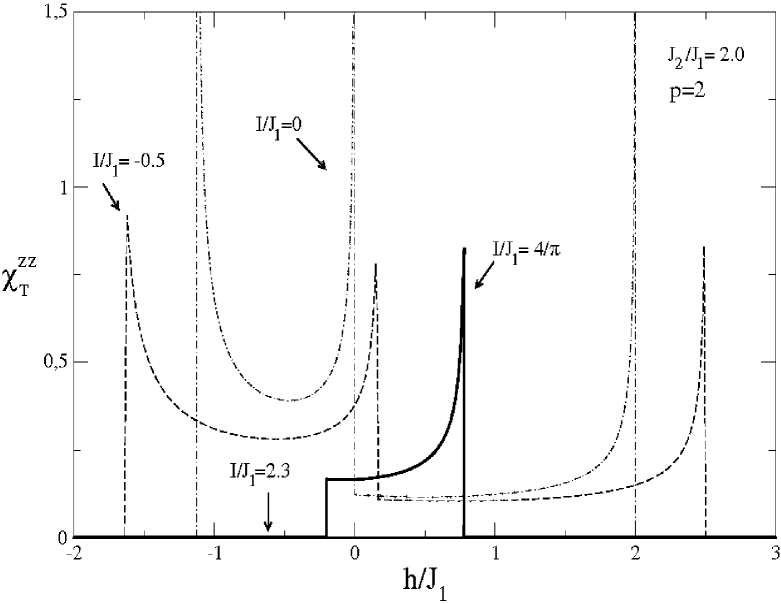
Figure 4: Isothermal susceptibility $\chi_{T}^{zz}$ as a function of $h/J_{1},$ for $p=2$, $J_{2}/J_{1}=2.0$ and different values $I/J_{1}.$

In Figs. 3 and 4 we present the magnetization and the isothermal susceptibility, respectively, and from their behavior we can conclude that for $I/J_{1}\leq 0$ the system undergoes second order transitions, and first-order transitions for $I/J_{1}>0.$

As can it be seen in Figs. 1 and 2, the number of transitions of first and second order depends on $J_{2},$ and it can also be shown that these transitions correspond to three phases for $0\leq J_{2}/J_{1}\leq 1/2,$and to four phases for $J_{2}/J_{1}>1/2.$ Following Titvinidze and JapararidzeTitvinidze 2003 , we can classify the intermediate phases, which are limited by the two saturate ferromagnetic phases, as quantum spin liquid phasesLee 2008 . As will be shown later, these spin liquid phases will be characterized by the spatial decay of the transversal static correlation function $\langle S_{j}^{x}S_{l}^{x}\rangle$ and by the modification of the oscillatory modulation of longitudinal static correlation function $\langle S_{j}^{z}S_{l}^{z}\rangle$.

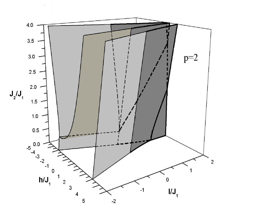
Figure 5: Global phase diagram for $p=2$ and $J_{2}/J_{1}\geq 0$, as a function of $h/J_{1}$ and $I/J_{1}$.

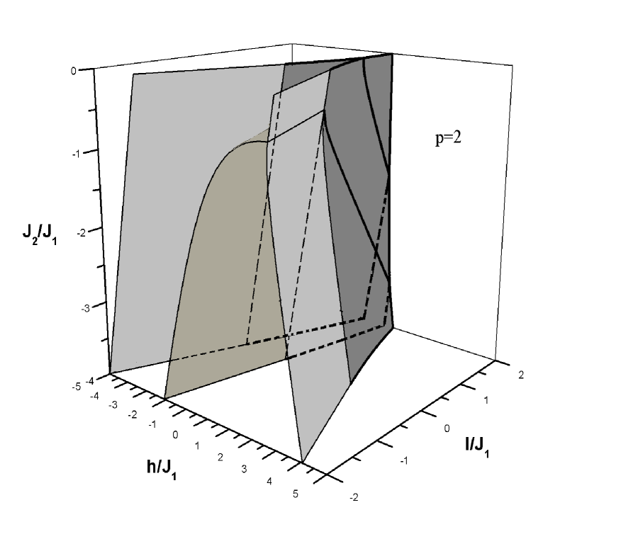
Figure 6: Global phase diagram for $p=2$ and $J_{2}/J_{1}\leq 0$, as a function of $h/J_{1}$ and $I/J_{1}$.

The global phase diagram for $p=2$ is shown in Figs. 5 and 6, for $J_{2}/J_{1}\geq 0$   and $J_{2}/J_{1}\leq 0,$ respectively. For $I\leq 0,$ the critical surfaces can be obtained explicitly and, for $J_{2}/J_{1}\geq 0,$ where there are four critical surfaces, which are given by the equations

$$\frac{J_{2}}{2J_{1}}-\frac{I}{J_{1}}-\frac{h}{J_{1}}+1=0,\text{ for }\frac{J_{2}}{J_{1}}\geq 0,$$ (32)

$$\frac{J_{2}}{2J_{1}}+\frac{I}{J_{1}}-\frac{h}{J_{1}}-1=0,\text{for }0\leq\frac{J_{2}}{J_{1}}\leq\frac{1}{2},$$ (33)

$$-\frac{J_{2}}{2J_{1}}-\frac{J_{1}}{4J_{2}}+\frac{I}{J_{1}}-\frac{h}{J_{1}}=0,\text{ for }\frac{J_{2}}{J_{1}}\geq\frac{1}{2},$$ (34)

$$\frac{J_{2}}{2J_{1}}-\frac{2IM_{1}^{z}}{J_{1}}-\frac{h}{J_{1}}+1=0,\text{ for }\frac{J_{2}}{J_{1}}\geq\frac{1}{2},$$ (35)

where

$$M_{1}^{z}=\frac{\arccos(\frac{J_{1}}{J_{2}}-1)}{\pi}-\frac{1}{2},$$ (36)

and for $J_{2}/J_{1}\leq 0$ there are four critical surfaces given by

$$-\frac{J_{2}}{2J_{1}}+\frac{I}{J_{1}}+\frac{h}{J_{1}}-1=0,\text{ for }\frac{J_{2}}{J_{1}}\leq 0,$$ (37)

$$-\frac{J_{2}}{2J_{1}}-\frac{I}{J_{1}}+\frac{h}{J_{1}}+1=0,\text{ for }-\frac{1}{2}\leq\frac{J_{2}}{J_{1}}\leq 0,$$ (38)

$$\frac{J_{2}}{2J_{1}}+\frac{J_{1}}{4J_{2}}-\frac{I}{J_{1}}+\frac{h}{J_{1}}=0,\text{ for }\frac{J_{2}}{J_{1}}\leq-\frac{1}{2},$$ (39)

$$-\frac{J_{2}}{2J_{1}}-\frac{2IM_{2}^{z}}{J_{1}}+\frac{h}{J_{1}}+1=0,\text{ for }\frac{J_{2}}{J_{1}}\leq-\frac{1}{2},$$ (40)

where

$$M_{2}^{z}=\frac{\arccos(\frac{J_{1}}{J_{2}}+1)}{\pi}-\frac{1}{2}.$$ (41)

The critical lines, shown in Figs. 1 and 2, can be obtained from Eqs. 32-36 for $\ J_{2}/J_{1}=0.2$ and $J_{2}/J_{1}=2.0,$ and from Eqs. 37-41 for $\ J_{2}/J_{1}=-0.2$ and $J_{2}/J_{1}=-2.0$.

It should be noted that for $J_{2}/J_{1}=1/2$ the critical surfaces meet at a bicritical lineLenilson 2005 given by

$$\frac{h}{J_{1}}=-\frac{3}{4}+\frac{I}{J_{1}}.$$ (42)

For $I>0,$ where the phase transitions are of first-order, critical surfaces are obtained numerically from the solution of the system

$$\left\{\begin{array}[c]{c}M_{it}^{z}-\frac{\varphi_{2t}^{i}-\varphi_{1t}^{i}}{\pi}+\frac{1}{2}=0,\\ M_{jt}^{z}-\frac{\varphi_{2t}^{j}-\varphi_{1t}^{j}}{\pi}+\frac{1}{2}=0,\\ f(M_{it}^{z})-f(M_{jt}^{z})=0,\end{array}\right.$$ (43)

where $\varphi_{2t}^{i}$ and $\varphi_{1t}^{i}$ are given by

$$\varphi_{1t}^{i}=\arccos\left[\frac{J_{1}+\sqrt{J_{1}^{2}+2J_{2}^{2}+4J_{2}\left(h_{t}+2IM_{it}^{z}\right)}}{2J_{2}}\right],\text{ }$$ (44)

$$\varphi_{2t}^{i}=\arccos\left[\frac{J_{1}-\sqrt{J_{1}^{2}+2J_{2}^{2}+4J_{2}\left(h_{t}+2IM_{it}^{z}\right)}}{2J_{2}}\right],$$ (45)

$M_{it}^{z},$ $M_{jt}^{z}$ are the values of the magnetization at the transition, with $i,$ $j=1,$ $2,$ $3,$ $4$  for $0\leq J_{2}/J_{1}\leq 1/2$, and with $i,$ $j=1,$ $2,$ $3,$ $4,$ $5,$ $6$ for $J_{2}/J_{1}\geq 1/2,$ and $f(M_{it}^{z})$ is given by Eq. (26). As in the case of second order transitions, the critical lines shown in the Fig. 1 are determined from the previous systems by considering $J_{2}/J_{1}=0.2$ and $J_{2}/J_{1}=2$.

For $J_{2}/J_{1}\geq 1/2,$ there are four critical surfaces and three of them, for $J_{2}/J_{1}=1/2,$ meet at a critical line which is determined by the following system of equations

$$\left\{\begin{array}[c]{c}M_{1t}^{z}-\frac{\varphi_{2t}^{1}-\varphi_{1t}^{1}}{\pi}+\frac{1}{2}=0,\\ M_{2t}^{z}-\frac{\varphi_{2t}^{2}-\varphi_{1t}^{2}}{\pi}+\frac{1}{2}=0,\\ M_{3t}^{z}-\frac{\varphi_{2t}^{3}-\varphi_{1t}^{3}}{\pi}+\frac{1}{2}=0,\\ f(M_{1t}^{z})-f(M_{3t}^{z})=0,\\ f(M_{2t}^{z})-f(M_{3t}^{z})=0,\end{array}\right.$$ (46)

where $f\left(M_{it}^{z}\right)$ is obtained from the Eq. (26), and with $i=1,$ $2,$ $3$ and $M_{3t}^{z}=-1/2.$ This is a triple line which meets the bicritical line at $I=0.$

A second triple line can be determined by imposing $M_{3t}^{z}=-1/2$ and $M_{4t}^{z}=1/2$ in the system

$$\left\{\begin{array}[c]{c}M_{2t}^{z}-\frac{\varphi_{2t}^{2}}{\pi}+\frac{1}{2}=0,\\ f(M_{2t}^{z})-f(M_{3t}^{z})=0,\\ f(M_{2t}^{z})-f(M_{4t}^{z})=0,\end{array}\right.$$ (47)

where $f(M_{2t}^{z}),$ and $\varphi_{2t}^{2}$ are given by Eqs. (26) and (45), which begins at the point $J_{2}/J_{1}=0,$ $h/J_{1}=0$ and $I/J_{1}=4/\pi,$ which has been obtained Gonçalves et al. Lenilson 2005 .

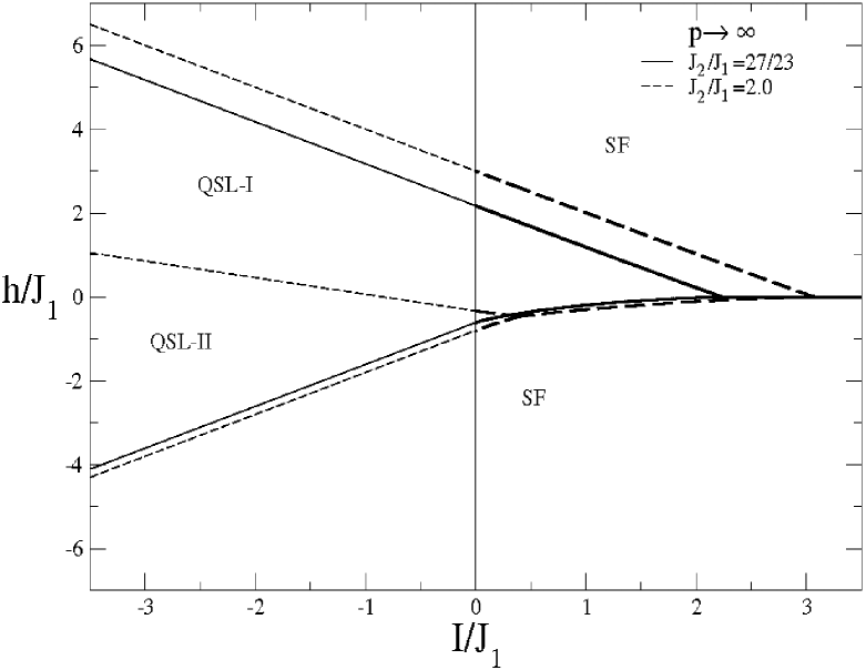
Figure 7: Phase diagram for the quantum transitions  as a function of the long-range interaction $I/J_{1}$ for $p\rightarrow\infty$ and $J_{2}/J_{1}=27/23,$ $2.0.$ For $J_{2}/J_{1}=27/23$ there are three phases, one spin liquid phase (QSL-I) and two saturated ferromagnetic phases(SF), and for $J_{2}/J_{1}=2.0,$ there are four phases, two spin liquid phases (QSL-I,QSL-II) and two saturated ferromagnetic phases(SF). The critical lines correspond to first-order phase transitions for $I/J_{1}>0$ and to second-order phase transitions for $I/J_{1}\leq 0.$

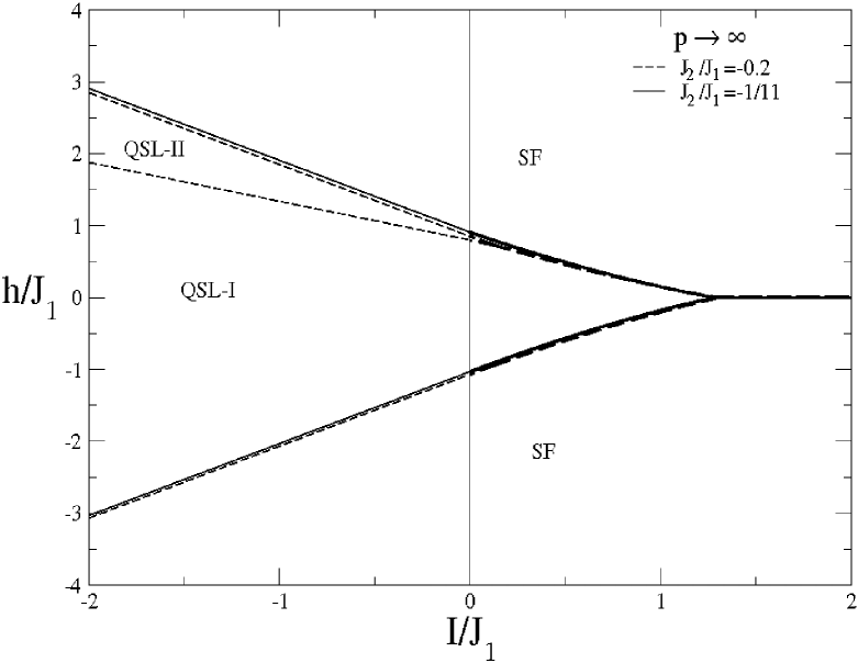
Figure 8: Phase diagram for the quantum transitions  as a function of the long-range interaction $I/J_{1}$ for $p\rightarrow\infty$ and $J_{2}/J_{1}=-0.2,-1/11.$ For $J_{2}/J_{1}=-0.2$ there are four phases, two spin liquid phases (QSL-I,QSL-II) and two saturated ferromagnetic phases(SF), and for $J_{2}/J_{1}=-1/11,$ there are three phases, one spin liquid phase (QSL) and two saturated ferromagnetic phases(SF). The critical lines correspond to first-order phase transitions for $I/J_{1}>0$ and to second-order phase transitions for $I/J_{1}\leq 0.$

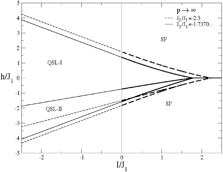
Figure 9: Phase diagram for the quantum transitions  as a function of the long-range interaction $I/J_{1}$ for $p\rightarrow\infty$ and $J_{2}/J_{1}=-2.5,-1.7370...$ For $J_{2}/J_{1}=-2.5$ there are four phases, two spin liquid phases (QSL-I,QSL-II) and two saturated ferromagnetic phases(SF), and for $J_{2}/J_{1}=-1.7370..,$ there are four phases, two spin liquid phases (QSL-I,QSL-II)) and two saturated ferromagnetic phases(SF) four phases which coexist in the quadruple point localized at $h/J_{1}=0,$ $I/J_{1}=1.7798...$ The functional of the free energy for this case is shown in Fig. 11. The critical lines correspond to first-order phase transitions for $I/J_{1}>0$ and to second-order phase transitions for $I/J_{1}\leq 0.$

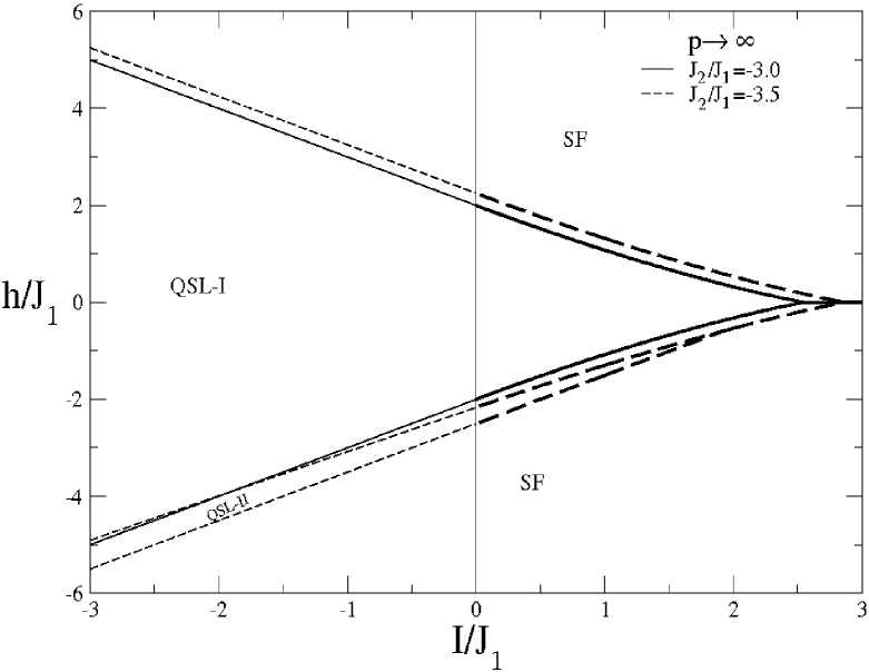
Figure 10: Phase diagram for the quantum transitions  as a function of the long-range interaction $I/J_{1}$ for $p\rightarrow\infty$ and $J_{2}/J_{1}=-3.5,-3.0.$ For $J_{2}/J_{1}=-3.5$ there are four phases, two spin liquid phases (QSL-I,QSL-II) and two saturated ferromagnetic phases(SF), and for $J_{2}/J_{1}=-3.0,$ there are three phases, one spin liquid phase (QSL-I) and two saturated ferromagnetic phases(SF).The critical lines correspond to first-order phase transitions for $I/J_{1}>0$ and to second-order phase transitions for $I/J_{1}\leq 0.$

For the special case $p\rightarrow\infty$, we can find the critical surfaces by using the same procedure used in the case $p=2$. In this case, due to many intersections of the critical surfaces, the global phase diagram becomes too complicated, as we will show below. Therefore, we will present some projections of the global diagram which contain the main characteristics of this diagram and are shown in Figs. 7-10.

In this case, the fermion excitation spectrum, obtained from Eq. (27), is given by

$$\epsilon_{q}\left(M^{z}\right)=J_{1}\cos(q)-J_{2}\left[\frac{2\cos\left(2q\right)+\cos\left(q\right)}{5+4\cos\left(q\right)}\right]+h+2IM^{z},$$ (48)

and from this result we can  determine the equations of the critical surfaces for $I/J_{1}\leq 0$ and $J_{2}/J_{1}\geq 0,$ which are

$$\frac{J_{2}}{J_{1}}-\frac{I}{J_{1}}-\frac{h}{J_{1}}+1=0,\text{ for }\frac{J_{2}}{J_{1}}\geq 0,$$ (49)

$$\frac{J_{2}}{3J_{1}}+\frac{I}{J_{1}}-\frac{h}{J_{1}}-1=0,\text{ for }0\leq\frac{J_{2}}{J_{1}}\leq\frac{27}{23},$$ (50)

$$\frac{5J_{1}-9J_{2}}{4J_{1}}+\sqrt{\frac{3J_{2}}{J_{1}}\left(\frac{J_{2}}{J_{1}}-1\right)}+\frac{I}{J_{1}}-\frac{h}{J_{1}}=0,\text{ for }\frac{J_{2}}{J_{1}}\geq\frac{27}{23},$$ (51)

$$\frac{J_{2}}{3J_{1}}-\frac{2IM_{1}^{z}}{J_{1}}-\frac{h}{J_{1}}-1=0,\text{ for }\frac{J_{2}}{J_{1}}\geq\frac{27}{23},$$ (52)

where

$$M_{1}^{z}=\frac{\arccos\left(\frac{11J_{2}-15J_{1}}{12J_{1}-12J_{2}}\right)}{\pi}-\frac{1}{2}.$$ (53)

Identically, we can show that for $I/J_{1}\leq 0$ and $J_{2}/J_{1}\leq 0$, the critical surfaces are

$$\frac{J_{2}}{J_{1}}-\frac{I}{J_{1}}-\frac{h}{J_{1}}+1=0,\text{ for }-\frac{1}{11}\leq\frac{J_{2}}{J_{1}}\leq 0,$$ (54)

$$\frac{J_{2}}{3J_{1}}+\frac{I}{J_{1}}-\frac{h}{J_{1}}-1=0,\text{ for }-3\leq\frac{J_{2}}{J_{1}}\leq 0,$$ (55)

$$\frac{5J_{1}-9J_{2}}{4J_{1}}-\sqrt{\frac{3J_{2}}{J_{1}}\left(\frac{J_{2}}{J_{1}}-1\right)}-\frac{I}{J_{1}}-\frac{h}{J_{1}}=0,\text{ for }\frac{J_{2}}{J_{1}}\leq-\frac{1}{11},$$ (56)

$$\frac{J_{2}}{J_{1}}-\frac{2IM_{2}^{z}}{J_{1}}-\frac{h}{J_{1}}+1=0,\text{ for }-3\leq\frac{J_{2}}{J_{1}}\leq-\frac{1}{11},$$ (57)

$$\frac{J_{2}}{J_{1}}+\frac{I}{J_{1}}-\frac{h}{J_{1}}+1=0,\text{ for }\frac{J_{2}}{J_{1}}\leq-3,$$ (58)

$$\frac{J_{2}}{3J_{1}}-\frac{2IM_{3}^{z}}{J_{1}}-\frac{h}{J_{1}}-1=0,\text{ for }\frac{J_{2}}{J_{1}}\leq-3,$$ (59)

where

$$M_{2}^{z}=\frac{\arccos\left(-\frac{7J_{2}+5J_{1}}{4J_{1}-4J_{2}}\right)}{\pi}-\frac{1}{2},$$ (60)

$$M_{3}^{z}=\frac{\arccos\left(\frac{-11J_{2}+15J_{1}}{12J_{1}-12J_{2}}\right)}{\pi}-\frac{1}{2}.$$ (61)

In this case there are three bicritical lines which are given by

$$\frac{h}{J_{1}}=-\frac{14}{23}+\frac{I}{J_{1}},\text{ at }J_{2}/J_{1}=27/23,$$ (62)

$$\frac{h}{J_{1}}=\frac{10}{11}-\frac{I}{J_{1}},\text{ at }J_{2}/J_{1}=-1/11,$$ (63)

$$\frac{h}{J_{1}}=-2+\frac{I}{J_{1}},\text{ at }J_{2}/J_{1}=-3.$$ (64)

For $I/J_{1}>0,$ as for the case $p=2$, the first order transition surfaces can be determined numerically and the triple lines are determined by following the same procedure adopted for $p=2.$

In Fig. 7 the phase diagram is shown for the positive region $J_{2}/J_{1}\geq 0,$ where there are four critical surfaces which are given by the Eqs (49-53). These critical surfaces meet at a bicritical line, which is given by Eq. 62.

The phase diagrams for the negative region $J_{2}/J_{1}\leq 0$ and for different values of $J_{2}/J_{1}$ are shown in Figs.8-10. In this case there are six critical surfaces, given by Eqs 54-59, which meet at bicritical lines given by the Eqs.(64-63). As we can see in Figs.8-10, the system presents in this case identical critical behavior to the one obtained for the case $p=2$, as far as the critical behavior is concerned. However, it is worth mentioning the appearance of quadruple point at $h/J_{1}=0,$ $J_{2}/J_{1}=-1.7370...,$ and $I/J_{1}=1.7798...,$which  is shown in Fig. 9 and is not present in the case $p=2$. The behavior of the functional of the Helmholtz free energy at this point is presented in Fig. 11.

We have also analysed the cases $p=3$ and $p=4$, for $I=0$, where the model presents new quantum spin liquid phases. Although in these cases there are no first-order transitions, we have restricted these analyses to the model without the long-range interaction, since the main purpose was to study appearance of new quantum spin liquid phases, which is mainly controlled by the multiple short-range interaction.

In Fig. 12 we show the phase diagram for the case $p=3,$ where the critical lines are given by

$$\frac{h}{J_{1}}=\frac{J_{2}}{4J_{1}}-1,$$ (65)

$$\frac{h}{J_{1}}=\frac{3J_{2}}{4J_{1}}+1,$$ (66)

$$\frac{h}{J_{1}}=\frac{1}{108}\left(\frac{13J_{2}-12J_{1}}{J_{1}}\right)^{\frac{3}{2}}-\frac{19J_{2}+36J_{1}}{108J_{1}},\text{ for }\frac{J_{2}}{J_{1}}\geq\frac{12}{13}\text{ or }\frac{J_{2}}{J_{1}}\leq-4,$$ (67)

$$\frac{h}{J_{1}}=-\frac{1}{108}\left(\frac{13J_{2}-12J_{1}}{J_{1}}\right)^{\frac{3}{2}}-\frac{19J_{2}+36J_{1}}{108J_{1}},\text{for }\frac{J_{2}}{J_{1}}\geq\frac{12}{13}\text{ or }\frac{J_{2}}{J_{1}}<0.$$ (68)

As it can be seen, there are six quantum spin liquid phases which, as we will show later, can be classified  in three different classes as far as the critical behavior is concerned.

The phase diagram for $p=4$ is shown in the Fig. 13, where the critical lines are given by

$$\frac{h}{J_{1}}=\frac{3J_{2}}{8J_{1}}-1,$$ (69)

$$\frac{h}{J_{1}}=\frac{7J_{2}}{8J_{1}}+1,$$ (70)

$$\frac{h}{J_{1}}=\frac{J_{2}}{16J_{1}}\left(\frac{R_{1}}{2}\right)^{4}-\frac{3J_{2}}{32J_{1}}\left(\frac{R_{1}}{2}\right)^{2}+\left(\frac{5J_{2}}{16J_{1}}-\frac{1}{2}\right)\left(\frac{R_{1}}{2}\right)-\frac{51J_{2}}{256J_{1}}-\frac{1}{4},$$ (71)

$$\frac{h}{J_{1}}=\frac{J_{2}}{16J_{1}}\left(\frac{R_{2}}{2}\right)^{4}-\frac{3J_{2}}{32J_{1}}\left(\frac{R_{2}}{2}\right)^{2}+\left(\frac{1}{2}-\frac{5J_{2}}{16J_{1}}\right)\left(\frac{R_{2}}{2}\right)-\frac{51J_{2}}{256J_{1}}-\frac{1}{4},$$ (72)

$$\frac{h}{J_{1}}=\frac{J_{2}R_{3i}^{4}}{J_{1}}-\frac{3J_{2}R_{3i}^{2}}{8J_{1}}+\left(\frac{5J_{2}}{8J_{1}}-1\right)R_{3i}-\left(\frac{51J_{2}}{256J_{1}}-\frac{1}{4}\right),$$ (73)

where $R_{1}\equiv$ $K^{\frac{1}{3}}+K^{-\frac{1}{3}},$ with

$$K \equiv(8J_{1}-5J_{2})/J_{2}+\sqrt{(64J_{1}^{2}-80J_{1}J_{2}+24J_{2}^{2})/J_{2}^{2}},\text{ \ \ }$$

$$J^{\prime} \equiv 16b/(b^{2}+10b+1)\text{ and }b=\left[(3+\sqrt{5})/2\right]^{3}\text{ for }J^{\prime}\leq J_{2}/J_{1}\leq 4/3,$$ (74)

$R_{2}\equiv S^{\frac{1}{3}}+S^{-\frac{1}{3}},$ with

$$S\equiv(5J_{2}-8J_{1})/J_{2}+\sqrt{(24J_{2}^{2}-80J_{1}J_{2}+64J_{1}^{2})/J_{2}^{2}},\text{ for }J_{2}/J_{1}<0\text{ or }J_{2}/J_{1}\geq 2,$$ (75)

and $R_{3i}\equiv\cos\left(\theta+\phi_{i}\right)/2,$ with

$$\theta=\arccos\left[(8J_{1}-5J_{2})/J_{2}\right]/3\text{ and }\phi_{i}=2\pi\left(i-1\right)/3,\text{ }i=1,2,3\text{ for }4/3\leq J_{2}/J_{1}\leq 2\text{.}$$ (76)

In this case, as for $p=3,$ the system presents six quantum spin liquid phases which can also be classified in three classes  as far as the critical behavior is concerned, as well as there exist only second order phase transitions.

IV STATIC SPIN CORRELATIONS

The static correlation function $\langle S_{j}^{z}S_{j+r}^{z}\rangle,$ in the thermodynamic limit, can be given bysiskens 1974 ; capel 1977 ; goncalves 1977 ,

$$\langle S_{j}^{z}S_{j+r}^{z}\rangle=\frac{Tr\left[\exp(-\beta\mathcal{H}^{-})S_{j}^{z}S_{j+r}^{z}\right]}{Tr\left[\exp(-\beta\mathcal{H}^{-})\right]},$$ (77)

where $\mathcal{H}^{-}$ is the Hamiltonian given in the Eq. (4).

After the introduction of the Fourier transform[Eq. (11)], $\mathcal{H}^{-}$ can be written in the form

$$\mathcal{H}^{-}={\displaystyle\sum\limits_{q}}\overline{\epsilon}_{q}\left(M^{z}\right)c_{q}^{\dagger}c_{q}+\frac{Nh}{2},$$ (78)

where $\overline{\epsilon}_{q}\left(M^{z}\right)$ is given by Eq. (22).

By introducing the fermion operators, we can write

$$S_{j}^{z}=\frac{1}{N}{\displaystyle\sum\limits_{qq^{\prime}}}\exp[ij(q-q^{\prime})]c_{q}^{\dagger}c_{q}-\frac{1}{2},$$ (79)

and from Eq. (79), by using the Wick’s theoremMattuck 1992 , the static correlation can be written as

$$\langle S_{j}^{z}S_{j+r}^{z}\rangle=\left[\frac{1}{N}{\displaystyle\sum\limits_{q}}\langle n_{q}\rangle-\frac{1}{2}\right]^{2}+\frac{1}{N^{2}}{\displaystyle\sum\limits_{qq^{\prime}}}\exp\left[i(q-q^{\prime})r\right](1-\langle n_{q^{\prime}}\rangle),$$ (80)

with

$$\langle n_{q}\rangle=\frac{1}{1+\exp\left[\overline{\epsilon}_{q}\left(M^{z}\right)\right]}.$$ (81)

From Eq. (80), we can obtain the static correlation function which, after some straightforward calculations, can be written as

$$\langle S_{j}^{z}S_{j+r}^{z}\rangle=\frac{1}{4}\left\{\left[\frac{1}{N}{\displaystyle\sum\limits_{q}}\tanh\left(\frac{\overline{\epsilon}_{q}}{2}\right)\right]^{2}-\left[\frac{1}{N}{\displaystyle\sum\limits_{q}}\cos(qr)\tanh\left(\frac{\overline{\epsilon}_{q}}{2}\right)\right]^{2}+\delta_{r0}\right\},$$ (82)

and, in the thermodynamic limit, in the form

$$\langle S_{j}^{z}S_{j+r}^{z}\rangle=\left[\frac{1}{2\pi}{\displaystyle\int\limits_{0}^{\pi}}\tanh\left(\frac{\overline{\epsilon}_{q}}{2}\right)dq\right]^{2}-\left[\frac{1}{2\pi}{\displaystyle\int\limits_{0}^{\pi}}\cos(qr)\tanh\left(\frac{\overline{\epsilon}_{q}}{2}\right)dq\right]^{2}+\frac{\delta_{r0}}{4}.$$ (83)

As it is well knownMcCoy 1971 , at $T=0$, the direct longitudinal correlation function of the short-range XY-model behaves asymptotically  as $\rho^{zz}(r)\equiv\langle S_{j}^{z}S_{j+r}^{z}\rangle-\left(M^{z}\right)^{2}\sim f(r)r^{-2},$ where $f(r)$ is an oscillatory function. A similar behavior can be found for the above expression[Eq.83] for the so-called quantum spin liquid phases, where the oscillatory factor $f(r)$ undergoes changes for different phases, as shown by Titvinidze and JaparadzeTitvinidze 2003 , for the case $p=2$ without long-range interaction.

In the presence of the long-range interaction, for $p=2$ and $I/J_{1}\leq 0,$ we have at most two multiple quantum spin liquid phases in the limit $T\rightarrow 0.$ For the first one phase the parameters satisfy the conditions

$$0 \leq\frac{J_{2}}{J_{1}}\leq\frac{1}{2},$$ (84)

$$-1+\frac{J_{2}}{2J_{1}}+\frac{I}{J_{1}} \leq\frac{h}{J_{1}}\leq 1+\frac{J_{2}}{2J_{1}}-\frac{I}{J_{1}},$$

or

$$\frac{J_{2}}{J_{1}} \geq\frac{1}{2},$$ (85)

$$-1+\frac{J_{2}}{2J_{1}}-\frac{2IM_{1}^{z}}{J_{1}} <\frac{h}{J_{1}}\leq 1+\frac{J_{2}}{2J_{1}}-\frac{I}{J_{1}},$$

where $M_{1}^{z}$ is given by Eq. (36), and from Eq. (83) we obtain

$$\rho^{zz}(r)\sim-\frac{\sin^{2}[q_{1}r]}{\pi^{2}r^{2}},$$ (86)

where

$$q_{1}=\arccos\left[\frac{J_{1}-y\left(M^{z}\right)}{2J_{2}}\right],$$ (87)

with

$$y\left(M^{z}\right)\equiv\sqrt{J_{1}^{2}+2J_{2}^{2}+4J_{2}\left(h+2IM^{z}\right)}.$$ (88)

For the second quantum spin liquid phase the parameters satisfy the conditions

$$\frac{J_{2}}{J_{1}} \geq\frac{1}{2},$$ (89)

$$-\frac{J_{2}}{2J_{1}}-\frac{J_{1}}{4J_{2}}+\frac{I}{J_{1}} \leq\frac{h}{J_{1}}\leq-1+\frac{J_{2}}{2J_{1}}-\frac{2IM_{1}^{z}}{J_{1}},$$

and, in this case, the asymptotic behavior of the direct correlation $\rho^{zz}(r)$ is given by

$$\rho^{zz}(r)\sim-\frac{\left\{\sin[q_{1}r]-\sin[q_{2}r]\right\}^{2}}{\pi^{2}r^{2}},$$ (90)

where $q_{1}$ is given by Eq. (87) and $q_{2}$ by

$$q_{2}=\arccos\left[\frac{J_{1}+y\left(M^{z}\right)}{2J_{2}}\right].$$ (91)

Therefore, $\rho^{zz}(r)$  shows a similar behavior to the case where the model does not contain long-range interactionTitvinidze 2003 .

The correlation length which diverges at the critical pointStanley 1971 , when we have a single phase, is associated to the period of the oscillation of $\rho^{zz}(r)$ and is defined by an analytical extension of its scaling form given byLima 1994

$$\rho^{zz}(n)\text{ }\sim\frac{F(in/\xi)}{n^{p}}.$$ (92)

When the system presents two phases between the saturated ferromagnetic phases, besides the correlation lengths $\xi_{1}$ there is an aditional one $\xi_{2},$ associated to the adjacent transitions and, in this case, we can define a further extension of the scaling form as

$$\rho^{zz}(n)\sim\frac{F(in/\xi_{1})+F(in/\xi_{2})}{n^{p}},$$ (93)

and define lenght of the system $\xi$ in the form

$$\xi=\xi_{1}+\xi_{2}.$$ (94)

Therefore, for the case where we have a single phase, by using Eq. (92), we can find from Eq. (86)

$$\frac{1}{\xi}=2\arccos\left[\left|\frac{J_{1}-y\left(M^{z}\right)}{2J_{2}}\right|\right],$$ (95)

which diverges at the critical points given by $h/J_{1}=1+J_{2}/2J_{1}-I/J_{1}$ and $h/J_{1}=-1+J_{2}/2J_{1}+I/J_{1}.$

On the other hand, for the case where we have two phases between the saturated ferromagnetic phases, by using Eqs. (93), (94) and, by using Eq. (90) we can find

$$\frac{1}{\xi}=\frac{\arccos\left[\left|\frac{J_{1}+y\left(M^{z}\right)}{2J_{2}}\right|\right]+\arccos\left[\left|\frac{J_{1}-y\left(M^{z}\right)}{2J_{2}}\right|\right]}{2\arccos\left[\left|\frac{J_{1}-y\left(M^{z}\right)}{2J_{2}}\right|\right]\left\{\arccos\left[\left|\frac{J_{1}+y\left(M^{z}\right)}{2J_{2}}\right|\right]-\arccos\left[\left|\frac{J_{1}-y\left(M^{z}\right)}{2J_{2}}\right|\right]\right\}},$$ (96)

which, as expected, diverges at the critical points $h/J_{1}=-1+J_{2}/2J_{1}-2IM_{1}^{z}/J_{1},$ $h/J_{1}=1+J_{2}/2J_{1}-I/J_{1}$ and $h/J_{1}=-J_{2}/2J_{1}-J_{1}/4J_{2}+I/J_{1},$ where $M^{z}$ is an intermidiate magnetization.

Although the results presented are for $p=2,$ it can be shown that the correlation lenght always diverges at all second order critical points irrespective of the value of $p,$ and for multiple transitions an aditional correlation length has to be introduced for each new phase presented by the system between the saturated ferromagnetic phases. Consequently, the scaling relation, given in Eq.(93), and teh correlation length of the system have to be redefined accordingly.

The transversal correlation function $\langle S_{j}^{x}S_{j+r}^{x}\rangle,$ given by the Toeplitz determinantLieb 1961

$$\langle S_{j}^{x}S_{j+r}^{x}\rangle=\frac{1}{4}\left(\begin{array}[c]{ccccc}\langle A_{1}B_{2}\rangle&\langle A_{1}B_{3}\rangle&\langle A_{1}B_{4}\rangle&...&\langle A_{1}B_{j+r+1}\rangle\\ \langle A_{2}B_{2}\rangle&\langle A_{2}B_{3}\rangle&\langle A_{2}B_{4}\rangle&...&\langle A_{2}B_{j+r+1}\rangle\\ \langle A_{3}B_{2}\rangle&\langle A_{3}B_{3}\rangle&\langle A_{3}B_{4}\rangle&...&\langle A_{3}B_{j+r+1}\rangle\\ \vdots&\vdots&\vdots&\ddots&\vdots\\ \langle A_{j}B_{j+r+2}\rangle&\langle A_{j}B_{l+3}\rangle&\langle A_{j}B_{l+4}\rangle&...&\langle A_{j}B_{j+r+1}\rangle\end{array}\right),$$ (97)

where

$$\langle A_{j}B_{l}\rangle=-\frac{1}{\pi}{\displaystyle\int\limits_{0}^{\pi}}\cos[q(j-l)]\tanh\left(\frac{\overline{\epsilon}_{q}\left(M^{z}\right)}{2}\right)dq,$$ (98)

can be evaluated numerically. This correlation, for the usual short-range XY-model and at $T=0$, behaves asymptotically  as $\langle S_{j}^{x}S_{j+r}^{x}\rangle\sim r^{-\frac{1}{2}}$McCoy 1971 . As in the case of the longitudinal correlation, the asymptotic behavior of the transversal correlation function $\langle S_{j}^{x}S_{j+r}^{x}\rangle$ also presents changes in its power law decay due to the presence of the multiple spin interaction. This result has been shown by Titvinidze and JaparadzeTitvinidze 2003 , in the case $p=2$ without long-range interaction, which classified these phases as spin liquid phases.

For the model with long-range interaction, the transversal static correlation, at $T=0$, was evaluated numerically from Eq. (97) by considering the maximum value of $r$ equal to $250,$ and the power decay determined by considering the scaling form $\langle S_{j}^{x}S_{l}^{x}\rangle\sim f(r)r^{-\overline{p}}$. The results for $p=2,$ are presented in Figs. 14 and 15 where the scaling forms are shown in the insets. The transversal correlation function for the quantum spin liquid I phase, presented in Fig. 14, the scaling behavior is given by $\langle S_{j}^{x}S_{j+r}^{x}\rangle\sim r^{-\frac{1}{2}},$ while for the quantum spin liquid II phase, presented in Fig. 15, it behaves as $\langle S_{j}^{x}S_{j+r}^{x}\rangle\sim f(r)r^{-1},$ where $f(r)$ is an oscillatory factor. These behaviors are identical to the ones obtained for the model without long-range interactionTitvinidze 2003 .We would also like to point out that identical results are obtained for the case $p\rightarrow\infty.$ This general result, which depends on the number of phases only, gives support to the classification of the intermediate phases as spin liquid phases.

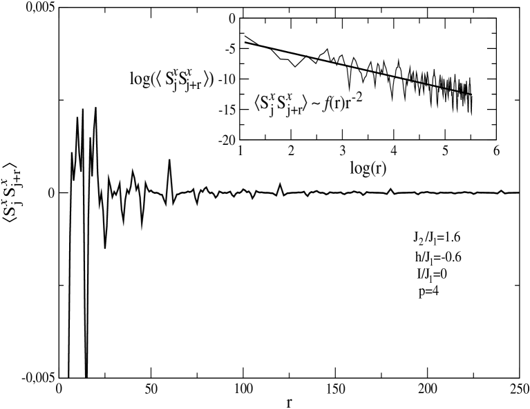
Figure 17: Static correlation function $\langle S_{j}^{x}S_{j+r}^{x}\rangle$as a function of $r$, for $p=4$, $h/J_{1}=-0.6,$ $J_{2}/J_{1}=1.6$ and $I/J_{1}=0.$ The inset shows the power law decay of the correlation characteristic of QSL-IV phase with the oscillatory modulation $f(r).$

The transversal static correlation was also calculated for $p=3,$ where there is a new quantum spin liquid phase, which can be identified in the phase diagram shown in Fig. 12. In this new phase, denominated quantum spin liquid III phase, its scaling behavior is given by $\langle S_{j}^{x}S_{j+r}^{x}\rangle\sim f(r)r^{-\frac{3}{2}},$ where the oscillatory behavior $f(r)$ is shown in Fig. 16. Finally, for $p=4,$ in the new phase denominated quantum spin liquid IV phase and shown in the phase diagram presented in Fig. 13, the scaling behavior of the transversal correlation function is given by $\langle S_{j}^{x}S_{j+r}^{x}\rangle\sim f(r)r^{-2}$, which is presented in Fig. 17.

It should be noted that, differently from the transversal correlation function, the spatial decay of the longitudinal correlation function does not depend on $\ p$.

V CRITICAL EXPONENTS

The critical exponents, at $T=0,$ associated with the magnetization, isothermal susceptibility, correlation length and the dynamic critical exponent $z,$ for $p=2$, can be evaluated analytically since the quantities of interest are known in closed form. Since these exponents are associated to second order transitions, our analysis will be initially restricted to $I\leq 0.$

Therefore, following Lima 1994 , we define the order parameter given by

$$\widetilde{M^{z}}\equiv M_{t}^{z}-M^{z},$$ (99)

where $M_{t}^{z}$ is the magnetization at the transition. This order parameter goes to zero at the second order transitions, and it is different from the one proposed by Titvinidze and JaparidzeTitvinidze 2003 . Then, from Eqs. (28), (87) and (88), we get

$$M^{z}=\frac{1}{\pi}\arccos\left[\frac{J_{1}-y\left(M^{z}\right)}{2J_{2}}\right]-\frac{1}{2},$$ (100)

and by expanding Eq. (100) up to second-order in $\widetilde{M^{z}}$, we obtain

$$\frac{\pi^{2}}{2}\left(\widetilde{M^{z}}\right)^{2}\cong\frac{J_{1}\left(h_{c}-h\right)}{J_{1}+2J_{2}},\text{ \ \ \ for \ }\frac{I}{J_{1}}=0,$$ (101)

and

$$\widetilde{M^{z}}\cong-\frac{J_{1}\left(h_{c}-h\right)}{2I},\text{ \ \ for \ }\frac{I}{J_{1}}<0.$$ (102)

From the Eqs. (101) and (102), and the scaling form $\widetilde{M^{z}}\sim\mid h_{c}-h$ $\mid^{\beta},$ we can conclude that the critical exponent $\beta$ is given by $\beta=\frac{1}{2},$ when $I/J_{1}=0$ and $\beta=1$ for $I/J_{1}<0$, respectively, showing  that the universality class has changed with the presence of the long-range interaction.

The isothermal susceptibility can be obtained from the Eq. (100), and is given by

$$\chi_{T}^{zz}=\frac{J_{1}}{\pi\sqrt{\left[y\left(M^{z}\right)\right]^{2}\left[1-\left(\frac{J_{1}-y\left(M^{z}\right)}{2J_{2}}\right)^{2}\right]}-2I}.$$ (103)

In the critical region, we have  $\chi_{T}^{zz}\sim\mid h_{c}-h$ $\mid^{\gamma},$ and from the previous expression we find that the critical exponent $\gamma$  is  equal to $\frac{1}{2},$ when $I/J_{1}=0,$ and  it is zero for $I/J_{1}<0$. Since at $T=0,$  $\gamma$  is identical to $\alpha,$ we can show that in both cases, namely, with or without long-range interaction  the exponents  $\beta,$ $\alpha$ and $\gamma$  satisfy the Rushbrook scaling relationStanley 1971 .

The critical exponent $\nu$ associated with the correlation length $\xi\sim\mid h_{c}-h\mid^{\nu}$, can be obtained from Eqs. (95) and (96). From these expressions we can immediately show that $\nu$ is  equal to $\frac{1}{2},$ when $I/J_{1}=0$ and  it is $1$ for $I/J_{1}<0$.

From the above results, by assuming the quantum hyperscaling relationContinentino 2001

$$2-\alpha=\nu\left(d+z\right),$$ (104)

where $d$ is the dimension of the system and $z$ the dynamic critical exponent,  we find  $z=1$ for $I<0,$ and $\ z=2$ for $I=0.$ Therefore, we can conclude that the system also presents a non-universal critical dynamical behavior.

For $I>0,$ following Continentino and FerreiraContinentino 2004 , we introduce a critical exponent associated to the free energy for the quantum first-order phase transition. Assuming the scaling form $f(h^{\pm})=f(h_{t})\pm E^{\pm}\mid h_{t}-h\mid^{2-\alpha}$ close to the field of transition $h_{t},$ since the free energy given in the Eq. (26) can be written as

$$f(\frac{h^{-}}{J_{1}})\cong f(\frac{h_{t}}{J_{1}})+M_{t}\mid\frac{h-h_{t}}{J_{1}}\mid,\text{ \ \ for \ }h<h_{t},$$ (105)

$$f(\frac{h^{+}}{J_{1}})\cong f(\frac{h_{t}}{J_{1}})-\frac{1}{2}\mid\frac{h-h_{t}}{J_{1}}\mid,\text{ \ \ for \ }h>h_{t},$$ (106)

we obtain $\alpha=1,$ which gives support to Continentino and Ferreira conjectureContinentino 2004 .

VI CONCLUSIONS

In this work we have considered the one-dimensional isotropic XY model with multiple spin interactions and uniform long-range interactions among the z components of the spin, in a transverse magnetic field. The solution of the model was obtained exactly for arbitrary $p,$ which characterizes the range of multiple spin interaction, and at arbitrary temperature. Explicit equations have been obtained for the functional of the Helmholtz free energy from which the equation of state can be determined numerically. The quantum critical behavior was studied in details for $p=2,3,4$ and $\infty,$ and the multiple phases presented by the model have been characterized by the asymptotic behavior of the static correlation  functions $\langle S_{j}^{z}S_{l}^{z}\rangle$ and $\langle S_{j}^{x}S_{l}^{x}\rangle.$ Irrespective of the value of $p$, the model presents first-order quantum transitions, when the long-range interaction is ferromagnetic, and second-order ones, when the long-range interaction is antiferromagnetic. Following  Titvinidze and JaparidzeTitvinidze 2003 , we have classified the intermediate phases, situated between saturated feromagnetic phases, as the so-called quantum spin liquid phases, which are induced by the extended interaction. For $p=2,$ the global phase diagram has been obtained as a function of the interaction parameters and the critical surfaces and multicritical lines determined exactly. The critical exponents have been obtained and it has been verified that they satisfy the Rushbrook relation $\alpha+$ 2$\beta+$ $\gamma=2$ (see e.g. ref.Stanley 1971 ) and the quantum hyperscaling relationContinentino 2001 $2-\alpha=\nu\left(d+z\right),$ and that the system presents a non-universal static and dynamic critical behavior. We have also shown that the free energy, close to first order transitions, satisfy the scaling form proposed by Continentino and FerreiraContinentino 2004 .

Finally, we would like to point out that it is of great importance the existence of multiple first order quantum transitions and multicritical lines (triple and quadruple lines) , which we have shown exactly to exist in the model, since we believe that they are related to the different mechanisms from which the first order phase transitions are driven, as discusssed by PfleidererPfleiderer 2005 .

VII ACKNOWLEDGMENTS

The authors would like to thank the Brazilian agencies Capes, CNPq and FAPEPI for partial financial support.

Figure 11: Functional of the free energy $f$ as a function of the magnetization $M^{z}$ for $p\rightarrow\infty$, $h/J_{1}=0,$ $I/J_{1}=1.7798...$ and $J_{2}/J_{1}=-1.7370...$ at the quadruple point.

Figure 12: Phase diagram for the quantum transitions as a function of $J_{2}/J_{1}$ for $p=3$ and $I/J_{1}=0$. All the transitions are of second-order and there are five phases, three spin liquid phase (QSL-I, QSL-II, QSL-III) and two saturated ferromagnetic phases (SF).

Figure 13: Phase diagram for the quantum transitions as a function of $J_{2}/J_{1}$ for $p=4$ and $I/J_{1}=0$. All the transitions are of second-order and there are five phases, three spin liquid phase (QSL-I, QSL-II, QSL-IV) and two saturated ferromagnetic phases (SF).

Figure 14: Static correlation function $\langle S_{j}^{x}S_{j+r}^{x}\rangle$as a function of $r$, for $p=2$, $h/J_{1}=2.0,$ $J_{2}/J_{1}=2.0$ and $I/J_{1}=-1.0.$ The inset shows the power law decay of the correlation characteristic of the QSL-I phase.

Figure 15: Static correlation function $\langle S_{j}^{x}S_{j+r}^{x}\rangle$as a function of $r$, for $p=2$, $h/J_{1}=-1.0,$ $J_{2}/J_{1}=2.0$ and $I/J_{1}=-1.0.$ The inset shows the power law decay of the correlation characteristic of QSL-II phase with the oscillatory modulation $f(r).$

Figure 16: Static correlation function $\langle S_{j}^{x}S_{j+r}^{x}\rangle$as a function of $r$, for $p=3$, $h/J_{1}=-0.15,$ $J_{2}/J_{1}=3.0$ and $I/J_{1}=0.$ The inset shows the power law decay of the correlation characteristic of QSL-III phase with the oscillatory modulation $f(r).$