Study of Decay Modes $B\to K_{0}^{*}(1430)\phi$

Within the framework of perturbative QCD approach based on $\mathbf{k_{T}}$ factorization, we investigate the charmless decay mode $B\to K_{0}^{*}(1430)\phi$. Under two different scenarios (S1 and S2) for the description of scalar meson $K_{0}^{*}(1430)$, we explore the branching fractions and related $CP$ asymmetries. Besides the dominant contributions from the factorizable emission diagrams, penguin operators in the annihilation diagrams could also provide considerable contributions. The central values of our predictions are larger than those from the QCD factorization in both scenarios. Compared with the experimental measurements of the BaBar collaboration, the result of neutral channel in the S1 agrees with experimental data, while the result of the charged one is a bit smaller than the data. In the S2 scenario, although the central value for the branching fractions of both channels are much larger than the data, the predictions could agree with the data due to the large uncertainties to the branching fractions from the hadronic input parameters. The $CP$ asymmetry in the charged channel is small and not sensitive to CKM angle $\gamma$. With the accurate data in near future from the various $B$ factories, these predictions will be under stringent tests.  
 
   PACS numbers:12.38.Bx, 11.10.Hi, 12.38.Qk, 13.25.Hw

1 Introduction

The $b\to ss\bar{s}$ transition, inducing many non-leptonic charmless $B$ meson decay processes such as $B\to K_{S}\phi$, $B\to K_{S}\eta(\eta^{\prime})$ and $B\to K^{*}\phi$, has attracted much interest because it serves as an ideal platform to probe the possible new physics (NP) beyond the standard model (SM). However, the kind of transition involving a scalar meson have more ambiguities due to intriguing but mysterious underlying nature of scalar mesons. In the spectroscopy study, there are two different scenarios to describe the scalar mesons. The scenario-1 (S1) is the naive 2-quark model: the nonet mesons below 1 GeV are treated as the lowest lying states, and the ones near 1.5 GeV are the first orbitally excited state. In the scenario-2 (S2), the nonet mesons near 1.5 GeV are viewed as the lowest lying states, while the mesons below 1 GeV may be viewed as exotic states beyond the quark model such as four-quark bound states. Under these two pictures, many $B\to SP$ modes, such as $B\to f_{0}K$, induced by $b\to ss\bar{s}$ transition have been calculated in both QCD factorization (QCDF) approach [1, 2] and perturbative QCD (PQCD) approach [3, 4, 5, 6]. Within proper regions for the input parameters, many theoretical results could agree with the experimental data.

In this work, we will study the $B\to K^{*}_{0}(1430)\phi$ decays in the perturbative QCD approach [7]. On the experimental side, the branching ratios of $B\to K_{0}^{*}(1430)\phi$ have been measured with good precision [8, 9]:

$${\cal B}(\overline{B}^{0}\to\overline{K}_{0}^{*0}(1430)\phi) = (4.6\pm 0.7\pm 0.6)\times 10^{-6}~{},$$ (1)

$${\cal B}(B^{\pm}\to K_{0}^{*\pm}(1430)\phi) = (7.0\pm 1.3\pm 0.9)\times 10^{-6}~{},$$ (2)

where the result for the neutral channel has been updated as [10]

$${\cal B}(\overline{B}^{0}\to\overline{K}_{0}^{*0}(1430)\phi) = (3.9\pm 0.5\pm 0.6)\times 10^{-6}~{}.$$ (3)

Compared with the $B\to K\phi$ decay [11]

$${\cal B}(\overline{B}^{0}\to\overline{K}^{0}\phi) = (8.3^{+1.2}_{-1.0})\times 10^{-6}~{},$$ (4)

$${\cal B}(B^{\pm}\to K^{\pm}\phi) = (8.30\pm 0.65)\times 10^{-6}~{},$$ (5)

we can see that the decay channels with a scalar meson in the final state, $B\to K_{0}^{*}(1430)\phi$, seem to have a bit smaller branching fractions. In Refs. [12, 13], the decay $\overline{B}^{0}\to\overline{K}_{0}^{*0}(1430)\phi$ has been studied within the framework of generalized factorization in which the non-factorizable effects are described by the parameter $N_{c}^{\rm eff}$, the effective number of colors. The predicted branching ratio (BR) varies from $10^{-7}$ to $10^{-5}$, depending on the different values for $N_{c}^{\rm eff}$. Without the information for non-factorizable effects, one cannot make a precise prediction of the BR. The QCDF calculation of this and other modes has also been presented in Ref. [14], and the predicted central value of ${\cal B}(\overline{B}^{0}\to\overline{K}^{*0}_{0}(1430)\phi)$ deviates from the experimental data, though it can be accommodated within large theoretical errors. It is necessary to analyze these channels in the PQCD approach with different treatments for the matrix elements of the four-quark operators, which is helpful to probe the structure of the scalar meson model-independently.

The layout of the present paper is as follows: In Sec. 2 we introduce the input parameters including the decay constants and light-cone distribution amplitudes. The factorization formulae in the perturbative QCD approach are given in Sec. 3. Numerical results and discussions are presented in Sec. 4. Summary of this work is also given in Sec. 4.

2 Input Parameters

In the $B$ meson rest frame, the $B$ meson momentum $P_{1}$, the $\phi$ meson momentum $P_{2}$, the longitudinal polarization vector $\epsilon_{L}$, and the kaon momentum $P_{3}$ are chosen, in light-cone coordinates, as

$$P_{1}=\frac{M_{B}}{\sqrt{2}}(1,1,{\bf 0}_{T})\;,\;\;\;P_{2} = \frac{M_{B}}{\sqrt{2}}(1-r_{K_{0}^{*}}^{2},r_{\phi}^{2},{\bf 0}_{T})\;,\;\;\;P_{3}=\frac{M_{B}}{\sqrt{2}}(r_{K_{0}^{*}}^{2},1-r_{\phi}^{2},{\bf 0}_{T})\;,\;\;\;$$

$$\epsilon = \frac{1}{\sqrt{2}r_{\phi}}(1-r_{K_{0}^{*}}^{2},-r_{\phi}^{2},{\bf 0}_{T})\;,$$ (6)

with the ratio $r_{\phi(K_{0}^{*})}=m_{\phi({K_{0}^{*}})}/M_{B}$, and $m_{\phi}$, $m_{K_{0}^{*}}$ being the $\phi$ meson mass and $K_{0}^{*}$ meson mass, respectively. The momentum of the light antiquark in the $B$ meson and the light quarks in the final mesons are denoted as $k_{1}$, $k_{2}$ and $k_{3}$ respectively. Using the intrinsic variables (momentum fractions and the transverse momentum), we can choose

$$k_{1}=(0,x_{1}P_{1}^{-},{\bf k}_{1T}),\quad k_{2}=(x_{2}P_{2}^{+},0,{\bf k}_{2T}),\quad k_{3}=(0,x_{3}P_{3}^{-},{\bf k}_{3T}).$$ (7)

The decay constants of scalar meson are defined by

$$\langle S(p)|\bar{q}_{2}\gamma_{\mu}q_{1}|0\rangle=f_{S}p_{\mu}\;,\;\langle S|\bar{q}_{2}q_{1}|0\rangle=m_{S}\bar{f}_{S},$$ (8)

where the decay constant $f_{S}$ of the vector current and $\bar{f}_{S}$ of the scalar current are related by equations of motion $\mu_{s}f_{S}=\bar{f}_{S}$, with $\mu_{s}=\frac{m_{S}}{m_{2}(\mu)-m_{1}(\mu)}$. The parameter $m_{S}$ is the mass of the scalar meson, and $m_{1}$, $m_{2}$ are the running current quark masses. Inputs of the scalar mesons in our calculation, including the decay constants, running quark masses and the Gegenbauer moments defined in the following, are quoted from Ref. [2].

For the scalar meson wave function, the twist-2 light-cone distribution amplitude (LCDA) $\phi_{S}(x)$ and twist-3 LCDAs $\phi_{S}^{s}(x)$ and $\phi_{S}^{\sigma}$ for the scalar mesons can be combined into a single matrix element:

$$\langle K_{0}^{*+}(p)|\bar{u}_{\beta}(z)s_{\alpha}(0)|0\rangle = \frac{1}{\sqrt{6}}\int^{1}_{0}dxe^{ixp\cdot z}\bigg{\{}p\!\!\!/\phi_{K^{*+}_{0}}(x)+m_{S}\phi^{S}_{K^{*+}_{0}}(x)+\frac{1}{6}m_{S}\sigma_{\mu\nu}p^{\mu}z^{\nu}\phi^{\sigma}_{K^{*+}_{0}}(x)\bigg{\}}_{\alpha\beta}$$ (9)

$$= \frac{1}{\sqrt{6}}\int^{1}_{0}dxe^{ixp\cdot z}\bigg{\{}p\!\!\!/\phi_{K^{*+}_{0}}(x)+m_{S}\phi^{S}_{K^{*+}_{0}}(x)+m_{S}(n\!\!\!/v\!\!\!/-1)\phi^{T}_{K^{*+}_{0}}(x)\bigg{\}}_{\alpha\beta},$$

where $v$ and $n$ are dimensionless vectors on the light cone, and $n$ is parallel with the moving direction of the scalar meson. The distribution amplitudes $\phi_{K^{*}_{0}}(x)$, $\phi^{S}_{K^{*}_{0}}(x)$ and $\phi^{\sigma}_{K^{*}_{0}}(x)$ are normalized as:

$$\int^{1}_{0}dx\phi_{K^{*}_{0}}(x)=\frac{f_{K^{*}_{0}}}{2\sqrt{6}},\,\,\,\,\,\,\int^{1}_{0}dx\phi^{S}_{K^{*}_{0}}(x)=\int^{1}_{0}dx\phi^{\sigma}_{K^{*}_{0}}(x)=\frac{\bar{f}_{K^{*}_{0}}}{2\sqrt{6}},$$ (10)

and $\phi^{T}_{K^{*}_{0}}(x)=\frac{1}{6}\frac{d}{dx}\phi^{\sigma}_{K^{*}_{0}}(x)$. For the $K^{*+}_{0}$ meson, the decay constant $f_{K^{*}_{0}}$ has the opposite sign with that of the $K^{*-}_{0}$ meson.

Under the conformal spin symmetry, the twist-2 LCDA $\phi_{K^{*}_{0}}(x)$ can be expanded as:

$$\phi_{K^{*}_{0}}(x,\mu) = \frac{\bar{f}_{K^{*}_{0}}(\mu)}{2\sqrt{6}}6x(1-x)\bigg{[}B_{0}(\mu)+\sum\limits^{\infty}_{m=1}B_{m}(\mu)C_{m}^{3/2}(2x-1)\bigg{]}$$ (11)

$$= -\frac{{f}_{K^{*}_{0}}(\mu)}{2\sqrt{6}}6x(1-x)\bigg{[}-1+\mu_{S}\sum\limits^{\infty}_{m=1}B_{m}(\mu)C_{m}^{3/2}(2x-1)\bigg{]},$$

where $B_{m}(\mu)$ and $C_{m}^{3/2}(x)$ are the Gegenbauer moments and Gegenbauer polynomials, respectively. The Gegenbauer moments $B_{1}$, $B_{3}$ of distribution amplitudes for $K^{*}_{0}$ and the decay constants have been calculated in the QCD sum rules [2] as

$$\mbox{S}\,{\rm 1} : \,\,\,\,B_{1}=0.58\pm 0.07,\;\;\;\;\;\;B_{3}=-1.20\pm 0.08,\;\;\;\;\;\;\bar{f}_{K^{*}_{0}}(1\mathrm{GeV})=-(300\pm 30)~{}~{}\mathrm{MeV};$$

$$\mbox{S}\,{\rm 2} : \,\,\,\,B_{1}=-0.57\pm 0.13,\;\;\;\;B_{3}=-0.42\pm 0.22,\;\;\;\;\;\;\bar{f}_{K^{*}_{0}}(1\mathrm{GeV})=(445\pm 50)~{}~{}\mathrm{MeV}.$$ (12)

All the above values are taken at $\mu=1$ GeV.

For the twist-3 LCDAs, they have been promoted in the Ref. [15] with large uncertainties, so we take the asymptotic form in our numerical calculation for simplicity:

$$\phi^{S}_{S}(x)=\frac{\bar{f}_{S}}{2\sqrt{6}},\,\,\,\,\,\phi^{T}_{S}(x)=\frac{\bar{f}_{S}}{2\sqrt{6}}(1-2x).$$ (13)

Up to twist-3 accuracy, the vector meson’s wave functions are collected as

$$\langle\phi(P_{2},\epsilon_{L})|\bar{s}_{\beta}(z)s_{\alpha}(0)|0\rangle = \frac{1}{\sqrt{6}}\int_{0}^{1}dxe^{ixP_{2}\cdot z}\left[m_{\phi}\not\!\epsilon^{*}_{L}\phi_{\phi}(x)+\not\!\epsilon^{*}_{L}\not\!P_{2}\phi_{\phi}^{t}(x)+m_{\phi}\phi_{\phi}^{s}(x)\right]_{\alpha\beta},$$ (14)

for longitudinal polarization. The distribution amplitudes can be parametrized as:

$$\phi_{\phi}(x) = \frac{3f_{\phi}}{\sqrt{6}}x(1-x)\left[1+a_{2\phi}^{||}C_{2}^{3/2}(2x-1)\right],\;$$

$$\phi^{t}_{\phi}(x) = \frac{3f^{T}_{\phi}}{2\sqrt{6}}(2x-1)^{2},$$

$$\phi^{s}_{\phi}(x) = \frac{3f_{\phi}^{T}}{2\sqrt{6}}(1-2x)~{},$$ (15)

with the Gegenbauer coefficient $a_{2\phi}^{||}(1{\rm GeV})=0.18\pm 0.08$ [16].

Since the $B$ meson is a pseudo-scalar heavy meson, the structure $(\gamma^{\mu}\gamma_{5})$ and $\gamma_{5}$ components remain as leading contributions. Then, $\Phi_{B}$ is written by

$$\Phi_{B}=\frac{i}{\sqrt{6}}\left\{(\not\!P_{B}\gamma_{5})\phi_{B}^{A}+\gamma_{5}\phi_{B}^{P}\right\},$$ (16)

where $P_{B}$ is the corresponding meson’s momentum, and $\phi_{B}^{A,P}$ are Lorentz scalar distribution amplitudes. As heavy quark effective theory leads to $\phi_{B}^{P}\simeq M_{B}\phi_{B}^{A}$, $B$ meson’s wave function can be expressed by

$$\phi_{B}(x,b)=\frac{i}{\sqrt{6}}\left[(\not\!P_{B}\gamma_{5})+M_{B}\gamma_{5}\right]\phi_{B}(x,b).$$ (17)

For the $B$ meson distribution amplitude, we adopt the model:

$$\phi_{B}(x,b)=N_{B}x^{2}(1-x)^{2}\exp\left[-\frac{1}{2}\left(\frac{xM_{B}}{\omega_{B}}\right)^{2}-\frac{\omega_{B}^{2}b^{2}}{2}\right]\;,$$ (18)

with the shape parameter $\omega_{B}=0.4$ GeV, which has been tested in many channels such as $B\to\pi\pi,K\pi$ [7]. The normalization constant $N_{B}=91.784$ GeV is related to the decay constant $f_{B}=190$ MeV. In the above model, $\phi_{B}$ has a sharp peak at $x\sim\bar{\Lambda}/M_{B}\sim 0.1$.

3 Analytical Formulae

In the PQCD approach, after the integration over $k_{1}^{+}$, $k_{2}^{+}$, and $k_{3}^{-}$, the decay amplitude for $B\to{K^{*}_{0}}\phi$ decay can be conceptually written as

$${\cal A} \sim \int\!\!dx_{1}dx_{2}dx_{3}b_{1}db_{1}b_{2}db_{2}b_{3}db_{3}$$ (19)

$$~{}~{}\times\mathrm{Tr}\left[C(t)\Phi_{B}(x_{1},b_{1})\Phi_{\phi}(x_{2},b_{2})\Phi_{K^{*}_{0}}(x_{3},b_{3})H(x_{i},b_{i},t)S_{t}(x_{i})\,e^{-S(t)}\right],$$

where $x_{i}$ are momenta fraction of light quarks in each meson. $\mathrm{Tr}$ denotes the trace over Dirac and color indices, $C(t)$ is the Wilson coefficient evaluated at scale $t$, and the hard kernel $H(k_{1},k_{2},k_{3},t)$ is the hard part and can be calculated perturbatively. And the function $\Phi_{M}$ is the wave function, the function $S_{t}(x_{i})$ describes the threshold resummation which smears the end-point singularities on $x_{i}$, and the last term, $e^{-S(t)}$, is the Sudakov form factor which suppresses the soft dynamics effectively.

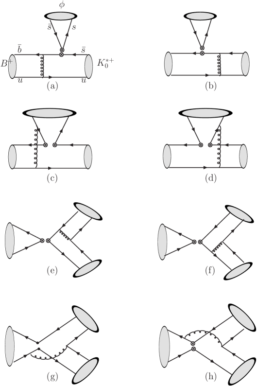
Figure 1: The leading order Feynman diagrams for $B^{+}\to K^{*+}_{0}\phi$ decay in PQCD approach

In the standard model, the effective weak Hamiltonian mediating flavor-changing neutral current transitions of the type $b\to s$ has the form:

$${\cal H}_{eff}={G_{F}\over\sqrt{2}}\Big{[}\sum\limits_{p=u,c}V_{pb}V^{*}_{ps}\Big{(}C_{1}O_{1}^{p}+C_{2}O_{2}^{p}\Big{)}-V_{tb}V^{*}_{ts}\sum\limits_{i=3}^{10,7\gamma,8g}C_{i}O_{i}\Big{]},$$ (20)

where the explicit form of the operator $O_{i}$ and the corresponding Wilson coefficient $C_{i}$ can be found in Ref. [17]. $V_{p(t)b}$, $V_{p(t)s}$ are the CKM matrix elements. According to effective Hamiltonian (20), we draw the lowest order diagrams of this channel in Fig. 1.

We first calculate the usual factorizable emission diagrams (a) and (b). If we insert the $(V-A)(V-A)$ or $(V-A)(V+A)$ operators in the corresponding vertexes, the amplitude associated to these currents is given as:

$$F_{e}=-8\pi C_{F}m_{B}^{4}f_{\phi}\int_{0}^{1}dx_{1}dx_{3}\int_{0}^{\infty}b_{1}db_{1}\,b_{2}db_{3}\,\phi_{B}(x_{1},b_{1})\\ \bigg{\{}\left[(1+x_{3})\phi_{K^{*}_{0}}(x_{3})+r_{K^{*}_{0}}(1-2x_{3})\left(\phi_{K^{*}_{0}}^{S}(x_{3})+\phi_{K^{*}_{0}}^{T}(x_{3})\right)\right]a(t_{a})E_{e}(t_{a})h_{e}(x_{1},x_{3},b_{1},b_{3})\\ +2r_{K^{*}_{0}}\phi_{K^{*}_{0}}^{S}({x_{3}})a(t_{b})E_{e}(t_{b})h_{e}(x_{3},x_{1},b_{3},b_{1})\bigg{\}}.$$ (21)

In the above formulae, $C_{F}=4/3$ is the group factor of the $SU(3)_{c}$ gauge group. We will use the same conventions for the functions $h_{e}$ and $E_{e}(t^{\prime})$ including the Sudakov factor and jet function as those in Ref. [18]. The $(S-P)(S+P)$ operator does not contribute to this decay as the emission particle is a vector particle. For the non-factorizable diagrams (c) and (d), all three meson wave functions are involved. For the $(V-A)(V-A)$ operators, the result can be read as:

$$M_{e}^{LL}=\frac{32\pi}{\sqrt{2N_{C}}}C_{F}m_{B}^{4}\int_{0}^{1}dx_{1}dx_{2}dx_{3}\int_{0}^{\infty}b_{1}db_{1}\,b_{2}db_{2}\,\phi_{B}(x_{1},b_{1})\phi_{\phi}(x_{2})\\ \bigg{\{}\left[(x_{2}-1)\phi_{K^{*}_{0}}(x_{3})+r_{K^{*}_{0}}x_{3}\bigg{(}\phi_{K^{*}_{0}}^{S}(x_{3})-\phi_{K^{*}_{0}}^{T}(x_{3})\bigg{)}\right]a(t_{c})E^{\prime}_{e}(t_{c})h_{n}(x_{1},1-x_{2},x_{3},b_{1},b_{2})\\ +\left[(x_{3}+x_{2})\phi_{K^{*}_{0}}(x_{3})-r_{K^{*}_{0}}x_{3}\left(\phi_{K^{*}_{0}}^{S}(x_{3})+\phi_{K^{*}_{0}}^{T}(x_{3})\right)\right]a(t_{d})E^{\prime}_{e}(t_{d})h_{n}(x_{1},x_{2},x_{3},b_{1},b_{2})\bigg{\}}\;.$$ (22)

For $(V-A)(V+A)$ and the $(S-P)(S+P)$ operators, the formulae are listed as:

$$M_{e}^{LR}=\frac{32\pi}{\sqrt{2N_{C}}}C_{F}m_{B}^{4}\int_{0}^{1}dx_{1}dx_{2}dx_{3}\int_{0}^{\infty}b_{1}db_{1}\,b_{2}db_{2}\,\phi_{B}(x_{1},b_{1})r_{\phi}\\ \bigg{\{}\bigg{[}(1-x_{2})\phi_{K^{*}_{0}}(x_{3})(\phi_{\phi}^{s}(x_{2})+\phi_{\phi}^{t}(x_{2}))+r_{K^{*}_{0}}\bigg{(}\phi_{\phi}^{s}(x_{2})\left[(x_{3}-x_{2}+1)\phi_{K^{*}_{0}}^{S}(x_{3})+(x_{3}+x_{2}-1)\phi_{K^{*}_{0}}^{T}(x_{3})\right]\\ -\phi_{\phi}^{t}(x_{2})\left[(x_{3}+x_{2}-1)\phi_{K^{*}_{0}}^{S}(x_{3})+(x_{3}-x_{2}+1)\phi_{K^{*}_{0}}^{T}(x_{3})\right]\bigg{)}\bigg{]}a(t_{c})E^{\prime}_{e}(t_{c})h_{n}(x_{1},1-x_{2},x_{3},b_{1},b_{2})\\ +\bigg{[}x_{2}\phi_{K^{*}_{0}}(x_{3})(\phi_{\phi}^{t}(x_{2})-\phi_{\phi}^{s}(x_{2}))-r_{K^{*}_{0}}\bigg{(}\phi_{\phi}^{s}(x_{2})\left[(x_{3}+x_{2})\phi_{K^{*}_{0}}^{S}(x_{3})+(x_{3}-x_{2})\phi_{K^{*}_{0}}^{T}(x_{3})\right]\\ +\phi_{\phi}^{t}(x_{2})\left[(x_{3}-x_{2})\phi_{K^{*}_{0}}^{S}(x_{3})+(x_{3}+x_{2})\phi_{K^{*}_{0}}^{T}(x_{3})\right]\bigg{)}\bigg{]}a(t_{d})E^{\prime}_{e}(t_{d})h_{n}(x_{1},x_{2},x_{3},b_{1},b_{2})\bigg{\}}\;,$$ (23)

$${\cal M}_{e}^{SP}=-\frac{32\pi}{\sqrt{2N_{C}}}C_{F}m_{B}^{4}\int_{0}^{1}dx_{1}dx_{2}dx_{3}\int_{0}^{\infty}b_{1}db_{1}\,b_{2}db_{2}\,\phi_{B}(x_{1},b_{1})\phi_{\phi}(x_{2})\\ \bigg{\{}\left[(1-x_{2}+x_{3})\phi_{K^{*}_{0}}(x_{3})-r_{K^{*}_{0}}x_{3}\bigg{(}\phi_{K^{*}_{0}}^{S}(x_{3})+\phi_{K^{*}_{0}}^{T}(x_{3})\bigg{)}\right]a(t_{c})E^{\prime}_{e}(t_{c})h_{n}(x_{1},1-x_{2},x_{3},b_{1},b_{2})\\ +\left[-x_{2}\phi_{K^{*}_{0}}(x_{3})+r_{K^{*}_{0}}x_{3}\left(\phi_{K^{*}_{0}}^{S}(x_{3})-\phi_{K^{*}_{0}}^{T}(x_{3})\right)\right]a(t_{d})E^{\prime}_{e}(t_{d})h_{n}(x_{1},x_{2},x_{3},b_{1},b_{2})\bigg{\}}\;,$$ (24)

Diagrams (e) and (f) are the factorizable annihilation diagrams, and the $(V-A)(V-A)$ kind of operators’ contributions are

$$F^{L}_{a}(a)=-8\pi C_{F}m_{B}^{4}f_{B}\int_{0}^{1}dx_{2}dx_{3}\int_{0}^{\infty}b_{2}db_{2}\,b_{3}db_{3}\ \\ \times\Bigg{\{}\Big{[}(x_{3}-1)\phi_{K^{*}_{0}}(x_{3})\phi_{\phi}(x_{2})-2r_{\phi}r_{K^{*}_{0}}\left((x_{3}-2)\phi_{K^{*}_{0}}^{S}(x_{3})-x_{3}\phi_{K^{*}_{0}}^{T}(x_{3})\right)\phi_{\phi}^{s}(x_{2})\Big{]}a(t_{e})E_{a}(t_{e})h_{a}(x_{2},1-x_{3},b_{2},b_{3})\\ +\Big{[}x_{2}\phi_{K^{*}_{0}}(x_{3})\phi_{\phi}(x_{2})-2r_{\phi}r_{K^{*}_{0}}\phi_{K^{*}_{0}}^{S}(x_{3})\left((x_{2}+1)\phi_{\phi}^{s}(x_{2})+(x_{2}-1)\phi_{\phi}^{t}(x_{2})\right)\Big{]}a(t_{f})E_{a}(t_{f})h_{a}(1-x_{3},x_{2},b_{3},b_{2})\Bigg{\}},$$ (25)

and the result from $(S-P)(S+P)$ currents is:

$$F^{SP}_{a}(a)=16\pi C_{F}m_{B}^{4}f_{B}\int_{0}^{1}dx_{2}dx_{3}\int_{0}^{\infty}b_{2}db_{2}\,b_{3}db_{3}\ \\ \times\Bigg{\{}\Big{[}2r_{\phi}\phi_{K^{*}_{0}}(x_{3})\phi_{\phi}^{s}(x_{2})+r_{K^{*}_{0}}(x_{3}-1)\left(\phi_{K^{*}_{0}}^{S}(x_{3})+\phi_{K^{*}_{0}}^{T}(x_{3})\right)\phi_{\phi}(x_{2})\Big{]}a(t_{e})E_{a}(t_{e})h_{a}(x_{2},1-x_{3},b_{2},b_{3})\\ -\Big{[}2r_{K^{*}_{0}}\phi_{K^{*}_{0}}^{S}(x_{3})\phi_{\phi}(x_{2})+r_{\phi}x_{2}\left(\phi_{\phi}^{t}(x_{2})-\phi_{\phi}^{s}(x_{2})\right)\phi_{K^{*}_{0}}(x_{3})\Big{]}a(t_{f})E_{a}(t_{f})h_{a}(1-x_{3},x_{2},b_{3},b_{2})\Bigg{\}}.$$ (26)

The last two diagrams in Fig. 1 are the non-factorizable annihilation diagrams, whose contributions are

$$M^{LL}_{a}(a)=\frac{32\pi}{\sqrt{2N_{C}}}C_{F}m_{B}^{4}\int_{0}^{1}dx_{1}dx_{2}dx_{3}\int_{0}^{\infty}b_{1}db_{1}\,b_{2}db_{2}\,\phi_{B}(x_{1},b_{1})\\ \bigg{\{}\bigg{[}x_{2}\phi_{K^{*}_{0}}(x_{3})\phi_{\phi}(x_{2})+r_{\phi}r_{K^{*}_{0}}\phi_{\phi}^{s}(x_{2})\left((x_{3}-x_{2}-3)\phi_{K^{*}_{0}}^{S}(x_{3})+(x_{3}+x_{2}-1)\phi_{K^{*}_{0}}^{T}(x_{3})\right)\\ -r_{\phi}r_{K^{*}_{0}}\phi_{\phi}^{t}(x_{2})\left((x_{3}+x_{2}-1)\phi_{K^{*}_{0}}^{S}(x_{3})+(x_{3}-x_{2}+1)\phi_{K^{*}_{0}}^{T}(x_{3})\right)\bigg{]}a(t_{g})E^{\prime}_{e}(t_{g})h_{na}(x_{1},x_{3},x_{2},b_{1},b_{2})\\ +\bigg{[}(x_{3}-1)\phi_{K^{*}_{0}}(x_{3})\phi_{\phi}(x_{2})-r_{\phi}r_{K^{*}_{0}}\phi_{\phi}^{t}(x_{2})\left((x_{3}+x_{2}-1)\phi_{K^{*}_{0}}^{S}(x_{3})+(-x_{3}+x_{2}+1)\phi_{K^{*}_{0}}^{T}(x_{3})\right)\\ -r_{\phi}r_{K^{*}_{0}}\phi_{\phi}^{s}(x_{2})\left((x_{3}-x_{2}-1)\phi_{K^{*}_{0}}^{S}(x_{3})-(x_{3}+x_{2}-1)\phi_{K^{*}_{0}}^{T}(x_{3})\right)\bigg{]}a(t_{h})E^{\prime}_{e}(t_{h})h^{\prime}_{na}(x_{1},x_{3},x_{2},b_{1},b_{2})\bigg{\}},$$ (27)

$$M^{LR}_{a}(a)=\frac{32\pi}{\sqrt{2N_{C}}}C_{F}m_{B}^{4}\int_{0}^{1}dx_{1}dx_{2}dx_{3}\int_{0}^{\infty}b_{1}db_{1}\,b_{2}db_{2}\,\phi_{B}(x_{1},b_{1})\\ \bigg{\{}\bigg{[}(2-x_{2})r_{\phi}\phi_{K^{*}_{0}}(x_{3})(\phi_{\phi}^{s}(x_{2})+\phi_{\phi}^{t}(x_{2}))+(x_{3}+1)r_{K^{*}_{0}}(\phi_{K^{*}_{0}}^{S}(x_{3})-\phi_{K^{*}_{0}}^{T}(x_{3}))\phi_{\phi}(x_{2})\bigg{]}a(t_{g})E^{\prime}_{e}(t_{g})h_{na}(x_{1},x_{3},x_{2},b_{1},b_{2})\\ +\bigg{[}x_{2}r_{\phi}\phi_{K^{*}_{0}}(x_{3})\left(\phi_{\phi}^{s}(x_{2})+\phi_{\phi}^{t}(x_{2})\right)-(x_{3}-1)r_{K^{*}_{0}}\left(\phi_{K^{*}_{0}}^{S}(x_{3})-\phi_{K^{*}_{0}}^{T}(x_{3})\right)\phi_{\phi}(x_{2})\bigg{]}a(t_{h})E^{\prime}_{e}(t_{h})h^{\prime}_{na}(x_{1},x_{3},x_{2},b_{1},b_{2})\bigg{\}}.$$ (28)

By combining the contributions from different diagrams with corresponding Wilson coefficients, one obtains the total decay amplitudes as

$${\cal A}(\overline{B}\to\overline{K}_{0}^{*0}(1430)\phi) = V_{tb}^{*}V_{ts}\Bigg{\{}F_{e}\left[a_{3}+a_{4}+a_{5}-\frac{1}{2}(a_{7}+a_{9}+a_{10})\right]$$ (29)

$$+M_{e}^{LL}\left[C_{3}+C_{4}-\frac{1}{2}C_{9}-\frac{1}{2}C_{10}\right]+M_{e}^{LR}\left[C_{5}-\frac{1}{2}C_{7}\right]+M_{e}^{SP}\left[C_{6}-\frac{1}{2}C_{8}\right]$$

$$+F_{a}^{LL}\left[a_{4}-\frac{1}{2}a_{10}\right]+F_{a}^{SP}\left[a_{6}-\frac{1}{2}a_{8}\right]$$

$$+M_{a}^{LL}\left[C_{3}-\frac{1}{2}C_{9}\right]+M_{a}^{LR}\left[C_{5}-\frac{1}{2}C_{7}\right]\Bigg{\}};$$

$${\cal A}(B^{+}\to K_{0}^{+*}(1430)\phi) = V_{tb}^{*}V_{ts}\Bigg{\{}F_{e}\left[a_{3}+a_{4}+a_{5}-\frac{1}{2}(a_{7}+a_{9}+a_{10})\right]$$ (30)

$$+M_{e}^{LL}\left[C_{3}+C_{4}-\frac{1}{2}C_{9}-\frac{1}{2}C_{10}\right]+M_{e}^{LR}\left[C_{5}-\frac{1}{2}C_{7}\right]+M_{e}^{SP}\left[C_{6}-\frac{1}{2}C_{8}\right]$$

$$+F_{a}^{LL}\left[a_{4}+a_{10}\right]+F_{a}^{SP}\left[a_{6}+a_{8}\right]+M_{a}^{LR}\left[C_{5}+C_{7}\right]+M_{a}^{LL}\left[C_{3}+C_{9}\right]\Bigg{\}}$$

$$-V_{ub}^{*}V_{us}\Bigg{\{}F_{a}^{LL}\left[C_{2}+\frac{1}{3}C_{1}\right]+M_{a}^{LL}C_{1}\Bigg{\}},$$

where $C_{i}$ are the Wilson coefficients for the four-quark operators and $a_{i}$ is defined as the combination of the Wilson coefficients:

$$a_{i}=C_{i}+\frac{C_{i\pm 1}}{N_{c}}$$ (31)

for an odd (even) value of $i$.

4 Numerical Results

The CKM phase $\gamma$ is defined via

$$V_{ub}=|V_{ub}|e^{-i\gamma},$$ (32)

and the CKM matrix elements that we used in the calculation are $|V_{ub}|=3.51\times 10^{-3}$, $|V_{us}|=0.225$, $|V_{cb}|=41.17\times 10^{-3}$ and $|V_{cs}|=0.973$ [19]. Moreover, we employ the unitary angle $\gamma=70^{\circ}$, the masses $m_{B}=5.28$ GeV and $m_{\phi}=1.02$ GeV. The longitudinal decay constant of $\phi$ could be extracted through the leptonic $\phi\to e^{+}e^{-}$ decay [20]

$$\Gamma(\phi\to e^{+}e^{-})=\frac{4\pi\alpha_{\rm em}^{2}e_{s}^{2}f_{\phi}^{2}}{3m_{\phi}},$$ (33)

which gives

$$f_{\phi} = 215~{}{\rm MeV}.$$ (34)

For the transverse decay constant, we use the recent Lattice QCD result [21] at 2 GeV

$$\frac{f_{\phi}^{T}}{f_{\phi}}=0.750\pm 0.008,$$ (35)

which corresponds to $f_{\phi}^{T}(1~{}\mathrm{GeV})=(178\pm 2)$ MeV. The ${\bar{B}}_{d}^{0}$ ($B^{-}$) meson lifetime $\tau_{B^{0}}=1.530$ ps ($\tau_{B^{-}}=1.638$ ps) [20].

With the above input parameters, the $B\to K^{*}_{0}$ form factors are given as

$$F_{1}(q^{2}=0)=-0.42^{+0.04+0.03-0.09}_{-0.04-0.03+0.07},\,\,\,\,\,\,\,\,\,\,\,\,S1;$$

$$F_{1}(q^{2}=0)=~{}~{}0.73^{+0.08-0.10+0.15}_{{-0.08}+0.09-0.12},\,\,\,\,\,\,\,\,\,\,\,\,S2;$$ (36)

where the first two uncertainties are from decay constants and the distribution amplitudes of the scalar meson, and the last uncertainty is from the $\omega_{B}$ in the distribution amplitude of $B$ meson. The decay constant in S2 is larger than that in S1, and contributions from the two terms proportional to $B_{1}$ and $B_{3}$ are constructive in S2 but destructive in S1. Thus the result for the form factor of $B\to K^{*}_{0}$ in S2 is almost twice larger than that in S1. Compared with the previous study of transition form factors [22], we can see that the present results for these form factors are a bit larger due to a weaker suppression for the endpoint region from the jet function $S_{t}(x)$.

The total decay amplitude for $B^{+}\to K_{0}^{*+}(1430)\phi$ can be written as:

$${\cal A}=V_{ub}^{*}V_{us}T-V_{tb}^{*}V_{ts}P=V_{ub}^{*}V_{us}T[1+ze^{i(\delta-\gamma)}],$$ (37)

where $z=|V_{tb}^{*}V_{ts}/V_{ub}^{*}V_{us}||P/T|$ and $\delta$ is the relative strong phase between tree diagrams ($T$) and penguin diagrams ($P$). The decay width is expressed as:

$$\Gamma(B^{+}\to K_{0}^{*+}(1430)\phi)=\frac{G_{F}^{2}}{32\pi M_{B}}|{\cal A}|^{2}=\frac{G_{F}^{2}}{32\pi M_{B}}|V_{ub}^{*}V_{us}T|^{2}[1+z^{2}+2z\cos(\delta-\gamma)].$$ (38)

Similarly, we can get the decay width for $B^{-}\to K_{0}^{*-}(1430)\phi$,

$$\Gamma(B^{-}\to K_{0}^{*-}(1430)\phi)=\frac{G_{F}^{2}}{32\pi M_{B}}|\overline{{\cal A}}|^{2},$$ (39)

where

$$\overline{{\cal A}}=V_{ub}V_{us}^{*}T-V_{tb}V_{ts}^{*}P=V_{ub}V_{us}^{*}T[1+ze^{i(\delta+\gamma)}].$$ (40)

From Eqs. (38) and (39), we get the averaged decay width:

$$\Gamma = \frac{G_{F}^{2}}{32\pi M_{B}}(|{\cal A}|^{2}/2+|\overline{\cal A}|^{2}/2)\hskip 28.45274pt$$ (41)

$$= \frac{G_{F}^{2}}{32\pi M_{B}}|V_{ub}^{*}V_{us}T|^{2}[1+z^{2}+2z\cos\gamma\cos\delta].$$

Using Eqs. (38) and (39), the direct $CP$ violation parameter is defined as

$$A_{CP}^{dir}=\frac{\Gamma(B^{-}\to K_{0}^{*-}(1430)\phi)-\Gamma(B^{+}\to K_{0}^{*+}(1430)\phi)}{\Gamma(B^{-}\to K_{0}^{*-}(1430)\phi)+\Gamma(B^{+}\to K_{0}^{*+}(1430)\phi)}=\frac{2z\sin\gamma\sin\delta}{1+2z\cos\gamma\cos\delta+z^{2}}.$$ (42)

Since only penguin operators work on the neutral decay mode, there is no direct $CP$ asymmetry in the decay $B^{0}\to K_{0}^{*0}(1430)\phi$, and its branching ratio can be calculated straightforwardly.

Using the parameters, we get the branching ratios in scenario 1 (S1):

$${\cal B}(B^{0}\to K_{0}^{*0}(1430)\phi) = 3.7\times 10^{-6},$$

$${\cal B}(B^{\pm}\to K_{0}^{*\pm}(1430)\phi) = 4.3\times 10^{-6},$$ (43)

while in scenario 2 (S2), the results are:

$${\cal B}(B^{0}\to K_{0}^{*0}(1430)\phi) = 23.6\times 10^{-6},$$

$${\cal B}(B^{\pm}\to K_{0}^{*\pm}(1430)\phi) = 25.6\times 10^{-6}.$$ (44)

From the above equations, we can see that the branching ratios in S2 are about 8 times larger than those in S1. There are three main reasons: (i) the larger decay constant in S2; (ii) contributions in emission diagrams from the two terms $B_{1}$ and $B_{3}$ are constructive in S2 but destructive in S1; (iii) the annihilation diagrams could cancel the contribution from the emission diagram. This kind of contribution in annihilation diagram is proportional to $B_{3}$. The larger value for $B_{3}$ in S1 will results in more sizable cancelation and the branching fractions are correspondingly reduced.

To be more explicit, we present values of the factorizable and non-factorizable amplitudes from the emission and annihilation topologies in Table. 1. As expected, the factorizable amplitudes are the largest, however the annihilation magnitudes are only few times smaller than that of factorizable emission diagrams. The non-factorizable amplitudes are down by a power of $\bar{\Lambda}/M_{B}\sim 0.1$ compared to the factorizable ones. The cancelation between the twist-2 and twist-3 contributions makes them even smaller. We demonstrate the importance of penguin enhancement in the Table. 1. It has been known that the RG evolution of the Wilson coefficients $C_{4,6}(t)$ dramatically increases as $t<m_{b}/2$, while that of $C_{1,2}(t)$ almost remains constant [17].

Table 1: Decay amplitudes for $B\to K_{0}^{*+}(1430)\phi$ ($\times 10^{-2}~{}\mbox{GeV}^{3}$)

$B^{+}\to K_{0}^{*+}(1430)\phi$		$F_{e}$	$M_{e}$	$F_{a}^{T}$	$F_{a}$	$M_{a}^{T}$	$M_{a}$
$S1$		$-13.4$	$-0.3+i0.0$	$-1.0-i4.0$	$8.1+i4.0$	$-2.8+i3.0$	$0.2+i0.0$
$S2$		$20.4$	$-0.8+i0.9$	$0.4+i0.8$	$-7.1-i12.0$	$9.3+i2.1$	$-0.3-i0.2$
$B^{0}\to K_{0}^{*0}(1430)\phi$		$F_{e}$	$M_{e}$	$F_{a}^{T}$	$F_{a}$	$M_{a}^{T}$	$M_{a}$
$S1$		$-13.4$	$-0.3+i0.0$	$0$	$8.3+i4.0$	$0$	$0.2-i0.1$
$S2$		$20.4$	$-0.8+i0.9$	$0$	$-7.2-i12.2$	$0$	$-0.5-i0.3$

In both scenarios, the branching ratio of $B^{+}\to K_{0}^{*+}(1430)\phi$ is a bit larger than that of $B^{0}\to K_{0}^{*0}(1430)\phi$, and the difference is from the tree contribution in $B^{+}\to K_{0}^{*+}(1430)\phi$. Since there exists interference between tree and penguin diagrams in the charged channel, the direct $CP$ asymmetry appears. So, we get the $CP$ asymmetry of $B^{\pm}\to K_{0}^{*\pm}(1430)\phi$ in the different scenarios as follows:

$${\cal A}_{dir}(B^{\pm}\to K_{0}^{*\pm}(1430)\phi) = 1.6\%,~{}~{}~{}~{}~{}~{}~{}~{}~{}~{}~{}~{}~{}~{}~{}S1$$

$${\cal A}_{dir}(B^{\pm}\to K_{0}^{*\pm}(1430)\phi) = 1.9\%.~{}~{}~{}~{}~{}~{}~{}~{}~{}~{}~{}~{}~{}~{}~{}S2$$ (45)

As the neutral channel as concerned, there is no $CP$ asymmetry as only penguin operators contribute to this channel.

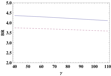
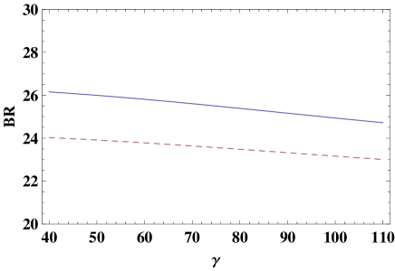
Figure 2: The dependence of the branching ratios($\times 10^{-6}$) for $B\to K_{0}^{*}(1430)\phi$ on the CKM angle $\gamma$, where the solid (dashed) curve is for charged (neutral) channel. The left (right) panel is plotted in S1(S2) scenario.

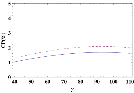
Figure 3: The dependence of the $CP$ asymmetry for $B^{\pm}\to K_{0}^{*}{\pm}(1430)\phi$ on the CKM angle $\gamma$, where the solid (dashed) curve is for S1 (S2) scenario

Although we set $\gamma=70^{\circ}$ in the above discussions, it is not measured accurately. In the following, we choose $\gamma$ as a free parameter and plot the branching ratios as a function of the angle $\gamma$ in both S1 and S2, as shown in the Fig. 2 and Fig. 3. As seen from the figures, we note that both the branching ratios and the $CP$ asymmetries in different scenarios are not sensitive to the phase $\gamma$. In the decay mode $B^{\pm}\to K_{0}^{*\pm}(1430)\phi$, the tree contribution only appears in the annihilation diagrams, which are suppressed compared with the emission diagrams. Moreover, the CKM element $|V_{ub}V_{us}|$ of tree diagrams is smaller than $|V_{tb}V_{ts}|$ of penguin diagrams. From this point of view, we can understand why the branching ratios and the $CP$ asymmetries are not sensitive to the $\gamma$.

In our calculation, the major uncertainties come from our lack of information about the scalar meson and heavy meson, involving the decay constants and the distribution amplitudes. The latter can be fitted from the well measured channels such as $B\to\pi\pi,K\pi$, the scalar one is not well ascertained. These uncertainties from the scalar meson can give sizable effects on the branching ratio, but the $CP$ asymmetries are less sensitive to these parameters. In this work, for instance, the twist-3 distribution amplitudes of the scalar mesons are taken as the asymptotic form, which may give large uncertainties. The characters of the scalar mesons need to be studied in future work. The another uncertainty comes from the sub-leading order contributions in PQCD approach, which have also been neglected in the calculation. In Ref. [23], parts of sub-leading order of $B\to\pi\pi,\pi K$ have been calculated, and the results show that corrections can change the penguin dominated processes, for example, the quark loops and magnetic-penguin correction decrease the branching ratio of $B\to\pi K$ by about $20\%$. We expect the similar size of uncertainty in the decays we analyzed , since they are also dominated by the penguin operators.

Here we give the results with the uncertainties as follows:

$${\cal B}(B^{0}\to K_{0}^{*0}(1430)\phi) = (3.7^{+0.8+0.1+3.7}_{-0.7-0.1-1.7})\times 10^{-6},$$

$${\cal B}(B^{-}\to K_{0}^{*-}(1430)\phi) = (4.3^{+0.9+0.1+4.3}_{-0.8-0.1-2.0})\times 10^{-6}\,\,\,\,\,\,\,\,\,\,\,\,S1;$$

$${\cal B}(B^{0}\to K_{0}^{*0}(1430)\phi) = (23.6^{+5.6+0.8+10.9}_{-5.0-0.6-5.8})\times 10^{-6},$$

$${\cal B}(B^{-}\to K_{0}^{*-}(1430)\phi) = (25.6^{+6.2+0.9+12.1}_{-5.4-0.8-6.5})\times 10^{-6}\,\,\,\,\,\,\,\,\,\,S2.$$ (46)

In the above results, the first uncertainty comes from the decay constants, and the second one is from the uncertainties of B1 (B3) in the amplitude distributions of the scalar meson. The last one comes from the uncertainty in the $B$ meson shape parameter $\omega=(0.40\pm 0.05)$ GeV. This kind of uncertainties is extremely large. The change of the shape parameter will mainly affect the emission diagram including the $B\to K^{*}_{0}$ form factor while the annihilation diagram, especially factorizable diagram, will not be affected sizably. Remember that the annihilation diagram could cancel part of contributions from emission diagram and thus the branching fractions are sizably changed due to the shape parameter.

In the QCD factorization approach, the results are listed as [14]:

$${\cal B}(B^{0}\to K_{0}^{*0}(1430)\phi) = (0.9^{+0.3+0.4+19.3}_{-0.3-0.3-0.5})\times 10^{-6},$$

$${\cal B}(B^{-}\to K_{0}^{*-}(1430)\phi) = (1.0^{+0.3+0.4+20.2}_{-0.3-0.3-0.5})\times 10^{-6}\,\,\,\,\,\,\,\,\,\,\,\,S1;$$

$${\cal B}(B^{0}\to K_{0}^{*0}(1430)\phi) = (16.9^{+6.2+1.7+51.8}_{-4.7-1.6-12.0})\times 10^{-6},$$

$${\cal B}(B^{-}\to K_{0}^{*-}(1430)\phi) = (17.3^{+6.2+1.7+52.4}_{-4.7-1.7-12.1})\times 10^{-6},\,\,\,\,\,\,\,\,\,S2.$$ (47)

Comparing two group of results, we note that our central values are much large than the results from QCDF in both two scenarios. It is mostly because that the form factor derived from Eq. (21) is larger than $F_{1}^{B\to K^{*}_{0}}(q^{2}=0)=0.21~{}(0.26)$ used in QCDF, which is calculated under S1 (S2) scenario in the covariant light-front model [24]. In addition, our results suffer from contribution from the annihilation diagrams, as demonstrated in the Table. 1. In fact, the contribution from annihilation can take the major uncertainties in the QCDF, as shown in the Eq. (4).

In the S1, for the neutral channel, our result is agree with experimental data well, but the result of the charged one is smaller than the data, though it is consistent within theoretical uncertainties. In the S2, both results are much larger than the data. The predictions in both scenarios suffer from very large uncertainties from the hadronic input parameters. Fortunately, most of these uncertainties will cancel out when we consider the ratio of branching fractions. It is convenient to define the ratio

$$R = \frac{\tau(B^{0})}{\tau(B^{+})}\frac{{\cal B}(B^{\pm}\to\phi K^{*\pm}_{0})}{{\cal B}(B^{0}\to\phi K^{*0}_{0})},$$ (48)

which is predicted as

$$R = 1.08\pm 0.01,\,\,\,\,\,\,\,\,\,\,\,\,S1;$$

$$R = 1.01\pm 0.01.\,\,\,\,\,\,\,\,\,\,\,\,S2;$$ (49)

Using the two experimental results, one can easily obtain the experimental data for this ratio

$$R_{\rm exp}=1.68\pm 0.51,$$ (50)

where all uncertainties are added in quadrature. For this ratio, the uncertainties from theoretical predictions are small while the experimental data has large uncertainties.

As a summary, we have studied the hadronic charmless decay mode $B\to K_{0}^{*}(1430)\phi$ within the framework of perturbative QCD approach in the standard model. Under two different scenarios, we explored the branching ratios and related $CP$ asymmetries. We find that besides the dominant contributions from the factorization emission diagrams, the penguin operators in annihilation can change the ratio remarkably. The central value of our results are larger than those from QCD factorization. Compared with experimental data from BaBar, in the S1, the result of neutral channel is agree with experimental data well, but the result of the charged one is a bit smaller than the data, though it is consistent within theoretical uncertainties. In the S2, both results are much larger than the data but the uncertainties are typically large. The ratio of branching fractions is found to have small uncertainties in the theoretical side.

References

[1]
H. Y. Cheng and K. C. Yang,
Phys. Rev. D 71, 054020 (2005)
[arXiv:hep-ph/0501253].
[2]
H. Y. Cheng, C. K. Chua and K. C. Yang,
Phys. Rev. D 73, 014017 (2006)
[arXiv:hep-ph/0508104].
[3]
C. H. Chen,
Phys. Rev. D 67, 014012 (2003)
[arXiv:hep-ph/0210028].
[4]
W. Wang, Y. L. Shen, Y. Li and C. D. Lu,
Phys. Rev. D 74, 114010 (2006)
[arXiv:hep-ph/0609082].
[5]
Y. L. Shen, W. Wang, J. Zhu and C. D. Lu,
Eur. Phys. J. C 50, 877 (2007)
[arXiv:hep-ph/0610380].
[6]
X. Liu, Z. Q. Zhang and Z. J. Xiao,
arXiv:0904.1955 [hep-ph].
[7]
Y. Y. Keum, H. N. Li and A. I. Sanda,
Phys. Rev. D 63, 054008 (2001)
[arXiv:hep-ph/0004173];
C. D. Lu, K. Ukai and M. Z. Yang,
Phys. Rev. D 63, 074009 (2001)
[arXiv:hep-ph/0004213].
[8]
B. Aubert et al. [BABAR Collaboration],
Phys. Rev. Lett. 98, 051801 (2007)
[arXiv:hep-ex/0610073].
[9]
B. Aubert et al. [BABAR Collaboration],
Phys. Rev. Lett. 101, 161801 (2008)
[arXiv:0806.4419 [hep-ex]].
[10]
B. Aubert et al. [The BABAR Collaboration],
Phys. Rev. D 78, 092008 (2008)
[arXiv:0808.3586 [hep-ex]].
[11]
E. Barberio et al. [Heavy Flavor Averaging Group (HFAG)],
arXiv:hep-ex/0603003. The updated results can be found at
www.slact.stanford.edu/xorg/hfag.
[12]
C. H. Chen, C. Q. Geng, Y. K. Hsiao and Z. T. Wei,
Phys. Rev. D 72, 054011 (2005)
[arXiv:hep-ph/0507012].
[13]
C. H. Chen and C. Q. Geng,
Phys. Rev. D 75, 054010 (2007)
[arXiv:hep-ph/0701023].
[14]
H. Y. Cheng, C. K. Chua and K. C. Yang,
Phys. Rev. D 77, 014034 (2008)
[arXiv:0705.3079 [hep-ph]].
[15]
C. D. Lu, Y. M. Wang and H. Zou,
Phys. Rev. D 75, 056001 (2007)
[arXiv:hep-ph/0612210].
[16]
P. Ball and G. W. Jones,
JHEP 0703, 069 (2007)
[arXiv:hep-ph/0702100].
[17] For a review, see G. Buchalla, A.J. Buras,
M.E. Lautenbacher, Rev. Mod. Phys. 68, 1125 (1996).
[18]
A. Ali, G. Kramer, Y. Li, C. D. Lu, Y. L. Shen, W. Wang and Y. M. Wang,
Phys. Rev. D 76, 074018 (2007)
[arXiv:hep-ph/0703162].
[19]
J. Charles et al. [CKMfitter Group],
Eur. Phys. J. C 41, 1 (2005)
[arXiv:hep-ph/0406184]. The updated results can be found at
http://ckmfitter.in2p3.fr/.
[20]C. Amsler et al. (Particle Data Group), Physics Letters B667, 1
(2008)
[21]
C. Allton et al. [RBC-UKQCD Collaboration],
Phys. Rev. D 78, 114509 (2008)
[arXiv:0804.0473 [hep-lat]].
[22]
R. H. Li, C. D. Lu, W. Wang and X. X. Wang,
Phys. Rev. D 79, 014013 (2009)
[arXiv:0811.2648 [hep-ph]].
[23]
H. n. Li, S. Mishima and A. I. Sanda,
Phys. Rev. D 72, 114005 (2005)
[arXiv:hep-ph/0508041];
H. n. Li and S. Mishima,
Phys. Rev. D 74, 094020 (2006)
[arXiv:hep-ph/0608277].
[24]
H. Y. Cheng, C. K. Chua and C. W. Hwang,
Phys. Rev. D 69, 074025 (2004)
[arXiv:hep-ph/0310359].