Validation of fluorescence transition probability calculations

Maria Grazia Pia, Paolo Saracco and Manju Sudhakar M. G. Pia and P. Saracco are with INFN Sezione di Genova, Via Dodecaneso 33, 16146 Genova, Italy (e-mail: MariaGrazia.Pia@ge.infn.it, Paolo.Saracco@ge.infn.it)M. Sudhakar is with INFN Sezione di Genova, Via Dodecaneso 33, 16146 Genova, Italy and Department of Physics, University of Calicut, India (e-mail: Manju.Sudhakar@ge.infn.it); she is on leave from ISRO Bangalore, IndiaManuscript received November16, 2009.

Abstract

A systematic and quantitative validation of the K and L shell X-ray transition probability calculations according to different theoretical methods has been performed against experimental data. This study is relevant to the optimization of data libraries used by software systems, namely Monte Carlo codes, dealing with X-ray fluorescence. The results support the adoption of transition probabilities calculated according to the Hartree-Fock approach, which manifest better agreement with experimental measurements than calculations based on the Hartree-Slater method.

Index Terms:

X-ray fluorescence, PIXE, Monte Carlo.

I Introduction

Analysis techniques using X-ray fluorescence are non-destructive methods to determine the elemental composition of material samples in a variety of applications, from planetary science to cultural heritage.

Software systems that deal with X-ray fluorescence, either for elemental analysis or Monte Carlo simulation, require accurate values of the physics parameters relevant for this process: the cross sections for the occurrence of the primary process creating a vacancy in the shell occupancy, the probability of radiative transitions once a vacancy has been created, and the energy of the emitted X-rays, which is determined by the binding energies of the atomic levels involved in the transition. These quantities usually derive from theoretical calculations, since experimental measurements cannot practically cover the entire range of physics conditions (target elements and incident particle characteristics) required by general-purpose software systems. The results of theoretical calculations are often tabulated in data libraries to avoid time-consuming computations of complex analytical formulae in software applications.

Calculations of radiative transition probabilities according to two different approaches, based on the Hartree-Slater and Hartree-Fock methods, are documented in the literature [1, 2, 3, 4]. Tabulations deriving from calculations with the Hartree-Slater method are collected in the Evaluated Atomic Data Library (EADL) [5], which is used by various Monte Carlo codes, including Geant4 [6, 7], for the simulation of X-ray fluorescence. GUPIX [8, 9], a specialized software system which is widely used for elemental analysis with PIXE (Particle Induced X-ray Emission) techniques, instead uses a database of K and L X-ray intensities based on Hartree-Fock calculations; however, this code and its databases are not freely available.

A systematic and quantitative evaluation of the relative merits of the two theoretical methods with respect to an extensive data sample is not available yet. This issue has been addressed by the study documented in this paper.

II Theoretical background

If one considers two energy levels in an atom, a perturbation to the system (like excitation or ionization) results in a superposition of the wavefunctions of the two levels; this superposition manifests itself as a probability amplitude or a charge cloud. This charge cloud oscillates with a frequency that is equal to the energy difference between the two states, causing the emission of radiation. If this disturbed system consists of only one electron, there is only the interaction between the nucleus and the electron to consider, and this can be described by a $1/r$ potential; for a many-electron system the repulsive force between the electron in question and the other electrons in the atom should also be included. This repulsive force is assumed to act centrally, like the $1/r$ force between the electron and the nuclues; combining these two, one can define the central field. The structure of this field is a function of the effective charge Z_eff of the screened nucleus and this screening, hence Z_eff is a function of the effective distance $r$ of the electron from the nucleus. This field can be determined by what is called the “self consistent field” method: an initial guess about the form of this field is made, which is used in the time-dependent Schrödinger equation to compute the wavefunctions; these are then used to calculate the charge distribution, and finally the potential set up by the charge distribution is determined. If the initial guess and the computed value do not match, the process is iterated.

This calculation was first made using the Hartree-Slater approach, where the electrons are assumed to move independently, with their mutual interaction accounted for by a mean field central potential; electrons, moreover, are treated relativistically and the effect of retardation is included [3]. However, within this approach initial and final wave functions are assumed to be identical, therefore missing some of the effects induced by the the Fermi statistics. The restricted Hartree-Fock approach was an obvious correction, giving a more accurate estimate of matrix elements of the transition operator between different subshells [3, 4]: the improvement comes essentially because there is room for a non vanishing overlap integral between initial and final single particle wave functions, which now are not assumed to be identical.

III Overview of the validation analysis

The validation study involved the comparison of fluorescence transition probabilities deriving from theoretical calculations against experimental measurements.

The theoretical and experimental data relevant to this study are available under various forms in the literature:

•

radiative emission rates, i.e. rates of decays of vacancies in a given shell accompanied by the emission of X-rays,
•

ratios of radiative emission rates, where the numerator and denominator in the ratios may concern an individual transition or a set of transitions,
•

probabilities of radiative transitions concerning individual shells, normalized over both radiative and non-radiative transitions.

The various data references cover different sets of transitions.

The different types of data were converted into a consistent representation to allow their comparison: transition probabilities over a common subset of transitions, listed in Table I.

The experimental data were extracted from the compilation of references in [10]; they were subject to selection and normalization procedures.

Theoretical values calculated according to the Hartree-Slater and Hartree-Fock approaches were taken from [1]-[4]; the selected subset of theoretical values corresponds to the transitions for which experimental data are reported in [10].

The radiative transition probabilities in EADL were processed similarly to the other theoretical tabulations.

For each transition, the theoretical and EADL transition probabilities as functions of the atomic number Z were compared with the experimental references using statistical methods to estimate their compatibility. The $\chi^{2}$ [12] test was performed to compare the data for each element. The null-hypothesis in the $\chi^{2}$ test assumed that the experimental data and those based on theoretical calculations derive from the same parent population; a 0.05 significance level was set to define the critical region of rejection of the null hypothesis.

Contingency tables were exploited to analyze the data resulting from the outcome of the $\chi^{2}$ test for each category of theoretical data. They were built based on the number of transitions that pass or fail the $\chi^{2}$ test, i.e. for which the p-value resulting from the test is greater or smaller than 0.05. In the analysis of the contingency tables the null hypothesis assumed the categories under evaluation to be equivalent regarding their accuracy to reproduce the experimental data. Contingency tables were analyzed with Fisher’s exact test [13]; as a cross-check, a $\chi^{2}$ test was also performed on the contingency tables, applying Yates’ correction [14] to account for the small number of entries in the tables.

IV Experimental data

An extensive compilation of experimental emission rates ratios for the K and L shell transitions is documented in [10]. To date it is still the most complete source of K and L shell experimental transition probability ratios; its relevance is confirmed by the fact that a recent database for X-ray spectroscopy [16], available from the NIST (National Institute of Standards) [17], is based on it for what concerns K and L radiative transition probabilities. Later measurements [18, 19] have been found consistent with the content of [10].

TABLE I: Radiative transition probabilities examined in this study

Transitions measured against a reference	Reference
K-L₂, K-M₂, K-M₃, K-M_4,5, K-N_2,3, K-N_4,5	K-L₃
L₁-M₂, L₁-N₂, L₁-N₃	L₁-M₃
L₂-M₁, L₂-N₄, L₂-O₄	L₂-M₄
L₃-M₁, L₃-M₄, L₃-N₁, L₃-N_4,5, L₃-O_4,5	L₃-M₅

IV-A Experimental sample

The original experimental measurements compiled in [10] were used for the validation of the theory.

Since [10] reports tabulations of fits to the data, but only bibliographical references and graphics of the original data, the experimental measurements and their uncertainties were retrieved from the original references, whenever they reported numerical values, or digitized from the published figures in cases where only graphical representations were available. The DigitizeIt [20] software was used for this purpose.

The uncertainties introduced by the digitization process were estimated by comparing the published numerical data, when available in the original references, to the corresponding digitized values. The average difference between published and digitized values was verified to be smaller than 2%, with the exception of the $L_{2}M_{1}$ transition, where 5% differences where observed. A further verification was performed on a selected data sample by comparing the values digitized by two software systems, DigitizeIt and Engauge [21]; the relative difference was smaller than 2%.

The experimental uncertainties for the emission rates vary from a few percent for the K-L₂ transition to approximately 25% for the L₂-O₄ transition. The uncertainties associated with some of the experimental data are not specified in the original references, nor in [10]; they were assumed in this study to be consistent with the average errors reported in other publications for the same kind of measurements and similar experimental conditions. In a few cases where such an inference was not possible due to the lack of comparable measurements, the data points deprived of any error estimate were not considered in the validation process.

Further evaluations were performed on the experimental collection to select a data sample suitable to be used as a reference for the validation of the theory. Those points not included in the data fits of [10] were discarded consistently with the arguments discussed in that reference. Multiple experimental data for the same element were combined; data points identified as outliers were discarded. Experimental data series looking largely inconsistent with the data collected by other experiments, were discarded too, as presumably affected by systematic errors.

IV-B Determination of transition probabilities

The data derived from this selection were subject to a preliminary treatment, to determine individual transition probabilities from the tabulated emission rate ratios. Since the experimental values reported in [10] are ratios relative to the strongest line in the series, the emission rate of the strongest line of each series was assumed to be one. Then the emission rates of each transition were normalized with respect to the sum of the emission rates of all the transitions in the series.

A method was devised to perform an indirect evaluation of experimental compatibility also for those transitions associated with the strongest line in each series, which have been taken as a reference in the probability ratios reported in [10]. The experimental reference probabilities for these transitions were calculated as the complement to unit total probability, taking into account the values associated with the other measured transitions.

The least square fits to the data tabulated in [10] and further interpolated in [16] were retained for most transitions; in a few cases ( $L_{1}N_{2}$ , $L_{2}N_{4}$ and $L_{2}O_{4}$ transitions) improved fits were found to better describe the data.

V Theoretical data

Emission rates deriving from Hartree-Slater and Hartree-Fock calculations, and EADL tabulations were subject to preliminary processing to assemble theoretical samples suitable to validation against the experimental data derived from [10]. The procedures adopted to retrieve theoretical data sets for the transitions listed in Table I, out of the theoretical tabulations available in the literature, are described in detail in [22].

V-A Emission rates based on the Hartree-Slater method

K and L X-ray emission rates, calculated by Scofield using the Hartree-Slater approach for elements with atomic number from 5 to 104, are tabulated in [2].

Only those transitions that are listed in Table I were selected for the validation process; the data were subject to normalization to obtain transition probabilities for each element relative to the subset of transitions under study (i.e. to each row in Table I).

V-B Emission rates based on the Hartree-Fock method

The K shell and L shell X-ray emission rates calculated by Scofield using the Hartree-Fock approach are tabulated in [3] and [4]. For the K shell, the emission rate ratios with respect to the strongest line in the series are listed for 50 elements with atomic number between 10 and 98; a limited number of emission rate ratios are reported.

The available data were transformed into transition probabilities; for each element the probabilities were normalized to 1 over each row of Table I.

For the L-shell emission rates, the tabulations in [4] are listed only for 21 elements in the range 18 $\leq$ Z $\leq$ 94. These have been computed from the Hartree-Fock based emission rates and then fitted with polynomials as a function of Z in [23]; the coefficients of these polynomials are reported in this reference for the different ranges of Z over which they are valid, for each transition. Using these coefficients, one can form equations to compute the intensities relative to the strongest line in the series; the absolute value of the strongest line of the series is also provided in [23], using which the individual transition probability for each transition can be computed for all Z.

V-C Transition probabilities in EADL

EADL includes binding energies of electrons for all subshells, the transition probabilities between subshells for emission of fluorescence photons and Auger electrons, and the energy of these emitted particles, for Z from 6 to 100. The transition probabilities are for all filled subshells in a neutral atom; it is assumed that the atomic relaxation process following the creation of an initial vacancy is independent of the ionizing radiation.

According to [5], the EADL radiative transition probabilities have been derived from Scofield’s Hartree-Slater calculations [1, 2]. Given the unclear documentation of the source of EADL tabulations, the validation process was meant not only to estimate the accuracy of this data library, but also to ascertain its content with respect to the published theoretical references.

The sum of the radiative and non-radiative transition probabilities listed in EADL for a shell (or subshell) adds to one for a particular element.

The transitions listed in EADL are extensive compared to those in [10]; only those transitions in EADL that are common with those in [10] were considered in the validation process, as listed in Table I.

VI Results

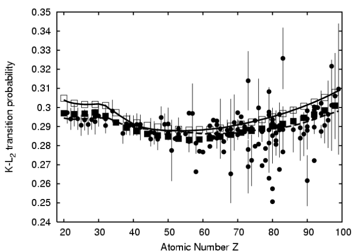
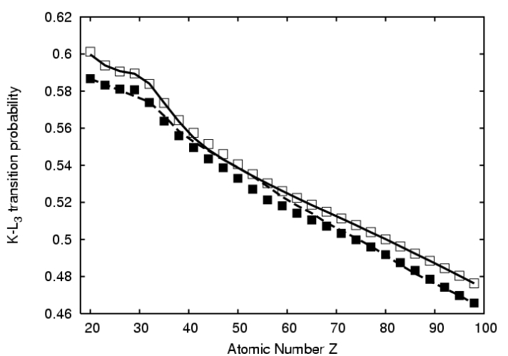
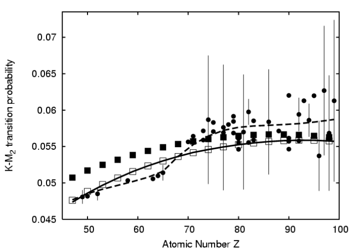
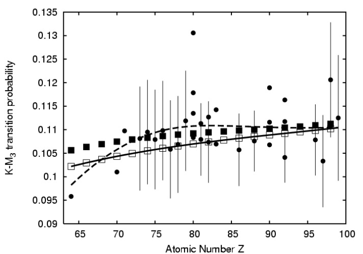
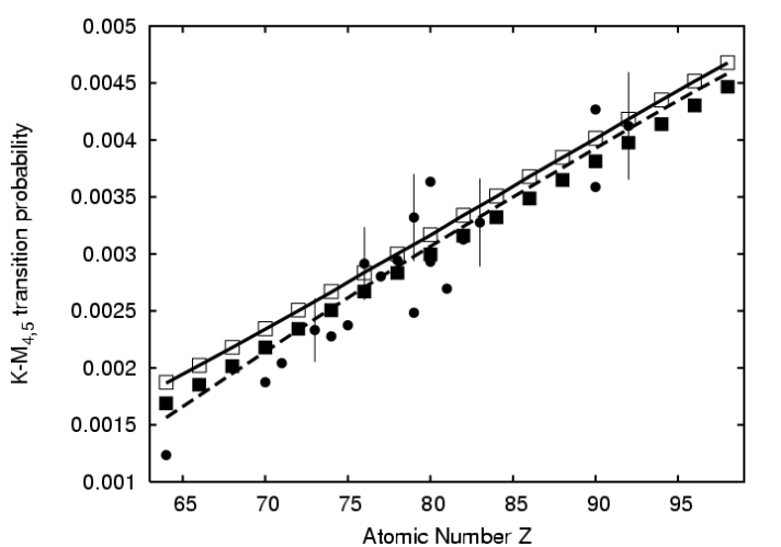
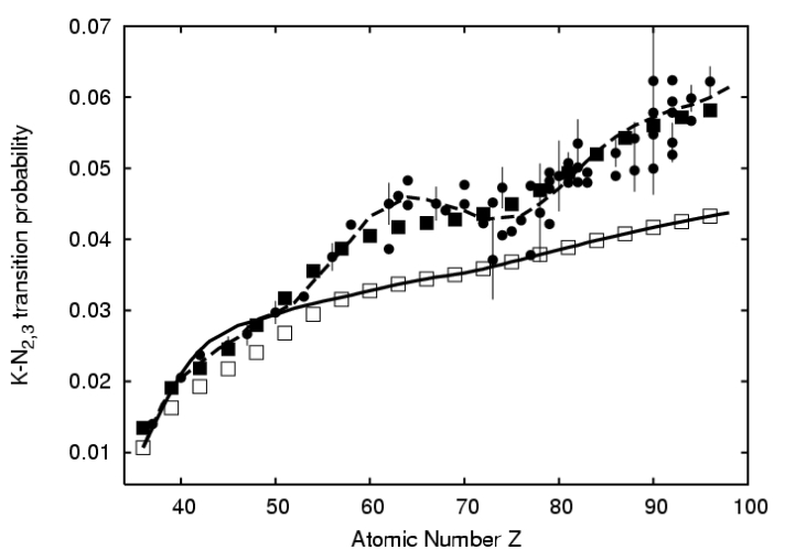
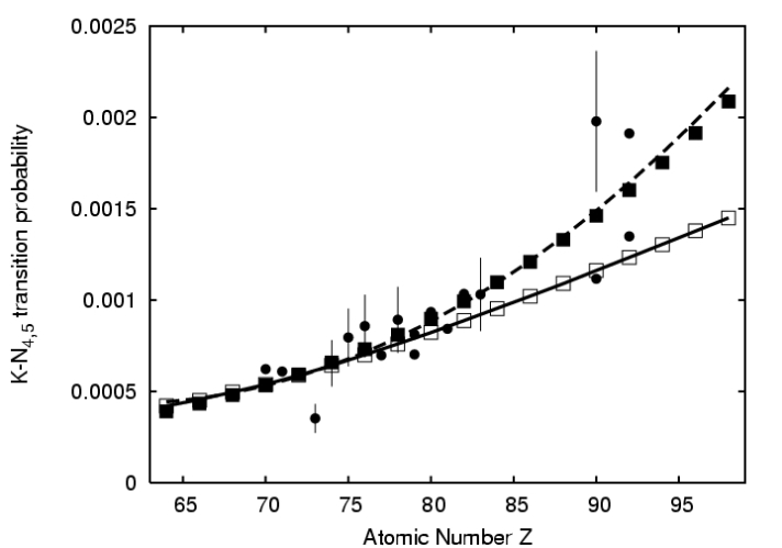
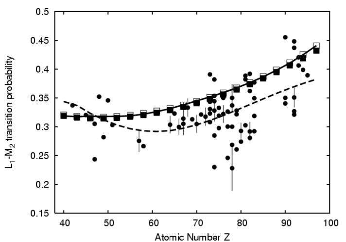
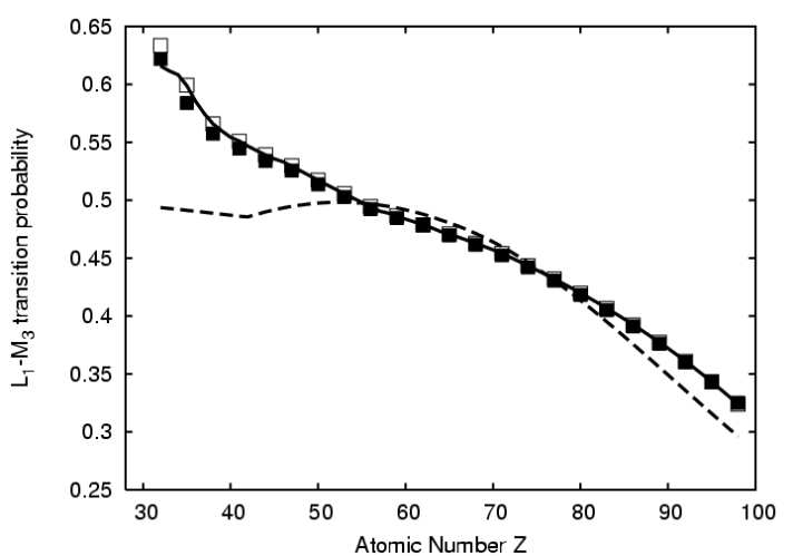
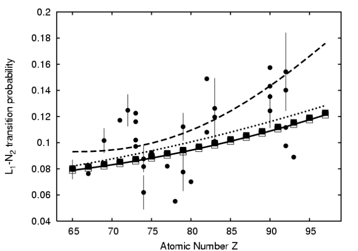
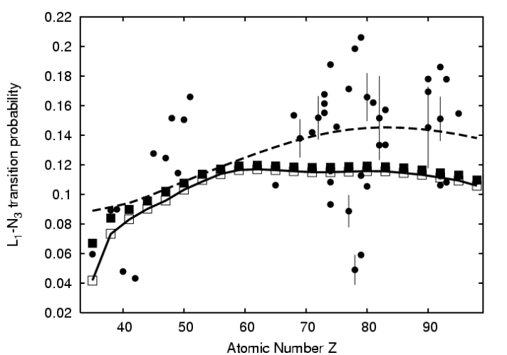
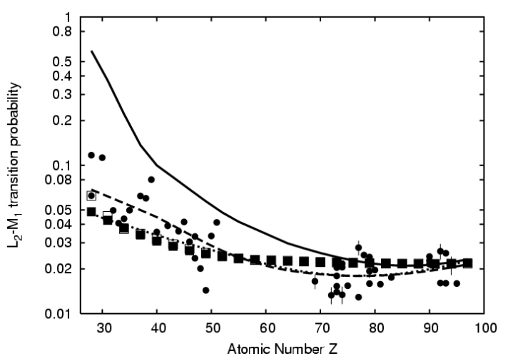
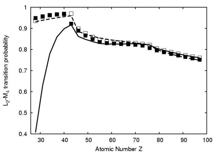
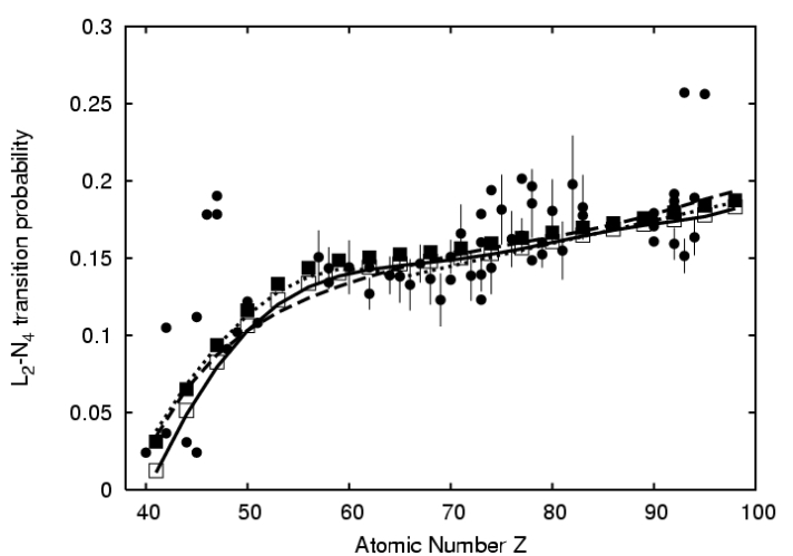
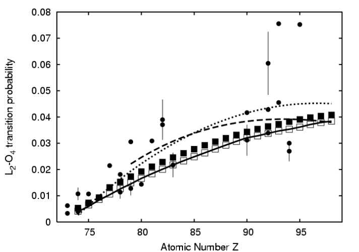
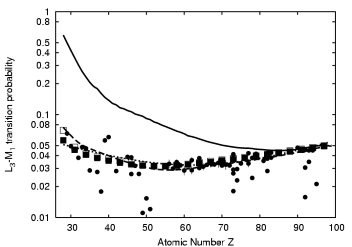
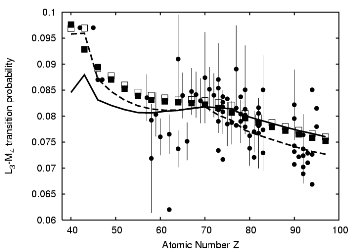
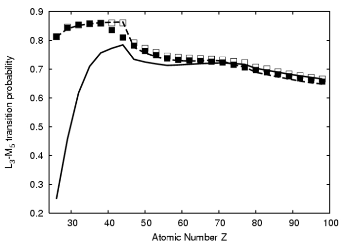
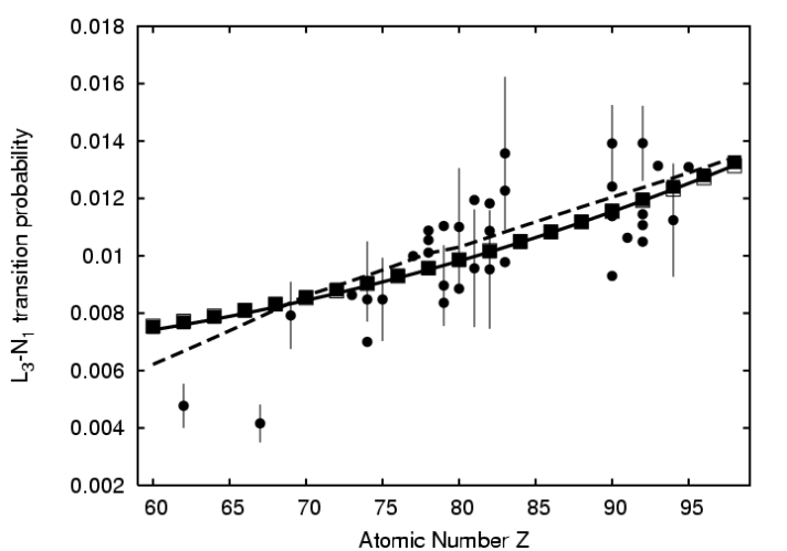
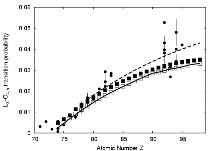
The transition probabilities for the K and L shells are shown in Fig. 1 through 21. The plots include the experimental data collected in [10], the Hartree-Slater and Hartree-Fock theoretical values, the corresponding EADL values, the fits to the experimental data as in [10] and [16], and the improved fits mentioned in section IV-B.

The p-values resulting from the $\chi^{2}$ tests are listed in Table II for each transition. The reference transitions in the probability ratios of [10] appear in italic.

TABLE II: p-values of the

\chi^{2}

test comparing transition probabilities from theoretical calculations against experimental data

Transition	Hartree	Hartree	EADL
	Slater	Fock
K-L₂	0.025	0.948	0.024
K-L₃	1	1	1
K-M₂	0.953	0.407	0.958
K-M₃	1	1	1
K-M_4,5	0.110	0.849	0.118
K-N_2,3	$<0.001$	0.717	$<0.001$
K-N_4,5	0.033	0.192	0.033
L₁-M₂	0.024	0.099	0.024
L₁-M₃	0.158	0.097	0.384
L₁-N₂	0.186	0.283	0.184
L₁-N₃	0.016	0.241	0.016
L₂-M₁	0.001	$<0.001$	$<0.001$
L₂-M₄	1	1	0
L₂-N₄	0.421	0.186	0.398
L₂-O₄	0.006	0.110	0.003
L₃-M₁	0.289	0.455	$<0.001$
L₃-M₄	0.721	0.880	0.831
L₃-M₅	1	1	1
L₃-N₁	1	1	1
L₃-N_4,5	0.002	0.277	$<0.001$
L₃-O_4,5	0.015	0.586	0.004

Assuming a confidence level of 95%, one can observe in Table II that the $\chi^{2}$ test rejects the null hypothesis of equivalence of the distributions subject to the test for a larger number of cases when comparing Hartree-Slater calculations to experimental data, with respect to comparisons involving Hartee-Fock ones. For transitions directly compared to experimental data (i.e. those listed in the left column of Table I), the null hypothesis is rejected in 53% of the test cases for the Hartree-Slater calculations, while it is rejected in 6% of the cases for the Hartree-Fock ones. The rejection of the null hypothesis occurs in a slightly larger number of the test cases (59%) for EADL with respect to Hartree-Slater calculations.

An analysis based on contingency tables was performed to estimate the statistical significance of the different accuracy observed with Hartree-Slater and EADL theoretical transition probabilities with respect to the Hartree-Fock ones. The contingency tables were based on the number of test cases which pass or fail the $\chi^{2}$ test, assuming a 95% confidence level for the rejection of the null hypothesis. The transitions involving direct comparisons to experimental data and the whole set of transitions were examined separately, to avoid introducing a possible bias in the conclusions due to different treatments of the data. The results are summarized in Table III.

TABLE III: Contingency tables comparing the accuracy of transition probability calculations

Transitions with direct experimental comparisons
$\chi^{2}$ test result	Hartree-Slater	Hartree-Fock
Pass	8	16
Fail	9	1
Fisher p-value	0.007
Yates $\chi^{2}$ p-value	0.008
$\chi^{2}$ test result	EADL	Hartree-Fock
Pass	7	16
Fail	10	1
Fisher p-value	0.002
Yates $\chi^{2}$ p-value	0.003
All transitions
$\chi^{2}$ test result	Hartree-Slater	Hartree-Fock
Pass	12	20
Fail	9	1
Fisher p-value	0.009
Yates $\chi^{2}$ p-value	0.011
$\chi^{2}$ test result	EADL	Hartree-Fock
Pass	10	20
Fail	11	1
Fisher p-value	0.001
Yates $\chi^{2}$ p-value	0.002

VII Comparative evaluations

The statistical results reported in the previous section are the basis for comparative evaluations.

VII-A Comparison of the accuracy of Hartree-Slater and Hartree-Fock calculations

The results of the statistical analysis in the previous section highlight a significant difference in the overall accuracy of the Hartree-Slater and Hartree-Fock calculations of radiative transition probabilities. While the more refined nature of the Hartree-Fock approach has been known from a theoretical perspective, this study provides a quantitative appraisal of the relative merits of the two calculations with respect to a large experimental sample.

More precise experimental data over a large number of elements would be needed to achieve firm conclusions of the relative accuracy of the two methods for individual atomic transitions.

VII-B Evaluation of EADL accuracy

Some differences are observed in Table II regarding the p-values related to the comparison of Hartree-Slater calculations and EADL against the experimental references. Small differences in the test statistics could derive from the data treatment described in the previous sections, which involves various manipulations to normalize the data to common references; however, large observed discrepancies should be ascribed to other reasons, which cannot be elucidated based on EADL documentation [5].

One can observe significant differences between the EADL values and the Hartree-Slater calculations for the L₂-M₁ (Fig. 12), L₂-M₄ (Fig. 13), L₃-M₁ (Fig. 16) and L₃-M₅ (Fig. 18) transitions; some discrepancies are also visible for L₃-M₄ (Fig. 17) and L₃-N_4,5 (Fig. 20). Discrepancies against experimental data were observed for some of these transitions in [24]. Similar differences were observed [11] between transition probabilities calculated by Geant4, which uses EADL in its atomic relaxation package [25], and the fitted data in [16].

Apart from these inconsistencies, the EADL content appears to reflect the Hartree-Slater calculations in [1, 2]; therefore the comments about the overall relative accuracy of Hartree-Slater calculations in the previous section hold for EADL too.

The results of this study suggest that a revision of EADL would be desirable to include more accurate radiative transition probabilities based on Hartree-Fock calculations.

VIII Conclusion

A systematic and quantitative validation of the existing theoretical models for computing K and L shell fluorescence transition probabilities was performed against an extensive collection of experimental data. The results, based on statistical methods, show that transition probabilities derived from Hartree-Fock calculations better represent the experimental measurements.

The EADL data library has been found not to represent the state-of-the-art for what concerns radiative transition probabilities. Based on the quantitative evidence obtained from this study, tabulations of Hartree-Fock values can be recommended as a replacement for the current radiative transition probabilities in EADL. Such an update of EADL would contribute to improve the accuracy of the Monte Carlo codes which use this data library for the simulation of X-ray fluorescence.

References

[1] J. H. Scofield, “Radiative Decay Rates of Vacancies in the K and L Shells”, Phys. Rev., vol. 179, no. 1, pp. 9-16, 1969.
[2] J. H. Scofield, “Relativistic Hartree-Slater Values for K and L X-ray Emission Rates”, Atom. Data Nucl. Data Tables, vol. 14, pp. 121-137, 1974.
[3] J. H. Scofield, “Exchange corrections of K X-ray emission rates”, Phys. Rev. A, vol. 9, no. 2, pp. 1041-1049, 1974.
[4] J. H. Scofield, “Hartree-Fock values of L X-ray emission rates”, Phys. Rev. A, vol. 10, no. 5, pp. 1507-1510, 1974.
[5] S. T. Perkins et al., “Tables and Graphs of Atomic Subshell and Relaxation Data Derived from the LLNL Evaluated Atomic Data Library (EADL)”, Z=1-100, UCRL-50400 Vol. 30, 1997.
[6] S. Agostinelli et al., “Geant4 - a simulation toolkit” Nucl. Instrum. Meth. A, vol. 506, no. 3, pp. 250-303, 2003.
[7] J. Allison et al., “Geant4 Developments and Applications” IEEE Trans. Nucl. Sci., vol. 53, no. 1, pp. 270-278, 2006.
[8] J. A. Maxwell et al., “The Guelph PIXE software package”, Nucl. Instrum. Meth. B, vol. 43, no. 2, pp. 218-230, 1989.
[9] J. A. Maxwell et al., “The Guelph PIXE software package II”, Nucl. Instrum. Meth. B, vol. 95, no. 3, pp. 407-421, 1995.
[10] S. I. Salem et al., “Experimental K and L Relative X-ray Emission Rates”, Atom. Data Nucl. Data Tables, vol. 14, pp. 91-109, 1974.
[11] A. Lechner et al., “Validation of Geant4 X-Ray Fluorescence Transitions - Validation of Geant4 electromagnetic models against calorimetry measurements in the energy range up to 1 MeV”, in Conf. Rec. 2008 IEEE Nucl. Sci. Symp..
[12] R. K. Bock and W. Krischer, “The Data Analysis BriefBook”, Ed. Springer, Berlin, 1998.
[13] R. A. Fisher, “On the interpretation of $\chi^{2}$ from contingency tables, and the calculation of P”, J. Royal Stat. Soc., vol. 85, no. 1, pp. 87-94, 1922.
[14] F. Yates, “Contingency tables involving small numbers and the $\chi^{2}$ test”, J. Royal Stat. Soc. Suppl., vol. 1, pp. 217-235, 1934.
[15] F. Yates, “Test of significance for 2 x 2 contingency tables”, J. Royal Stat. Soc. A, vol. 147, no. 3, pp. 426-463, 1984.
[16] W. T. Elam et al., “A new atomic database for X-ray spectroscopic calculations”, Radiat. Phys. Chem., vol. 63, pp. 121-128, 2002.
[17] W. T. Elam, FP compilation [Online]. Available: http://www.cstl.nist.gov/acd/839.01/ElamDB12.zip.
[18] M. Dost et al., “K-shell ionisation cross sections and relative X-ray emission rates of Sn, Ho, Tm, Au, Pb and Bi bombarded with 9-155 MeV alpha particles”, J. Phys. B, vol. 14, pp. 3153-3161, 1981.
[19] A. Raulo et al., “L₃-subshell x-ray emission rates for Dy and Ho”, J. Phys. B, vol. 40, pp. 2739-2746, 2007.
[20] I. Borman, DigitizeIt [Online]. Available: http://www.digitizeit.de.
[21] M. Mitchell, Engauge Digitizer [Online]. Available: http://digitizer.sourceforge.net.
[22] M. G. Pia et al., “Validation of radiative transition probability calculations”, IEEE Trans. Nucl. Sci., vol. 56, no. 6, Dec. 2009.
[23] S. Puri, “Relative intensities for L_i (i = 1-3) and M_i (i = 1-5) subshell X-rays”, Atom. Data Nucl. Data Tables, vol. 93, pp. 730-741, 2007.
[24] R. D. Bonetto, A. C. Carreras, J. Trincavelli, and G. Castellano, “L-shell radiative transition rates by selective synchrotron ionization”, J. Phys. B, vol. 37, pp. 1477-1488, 2004.
[25] S. Guatelli et al., “Geant4 Atomic Relaxation”, IEEE Trans. Nucl. Sci., vol. 54, no. 3, pp. 585-593, 2007.

Refer to caption — Figure 1: K-L₂ transition probability versus Z: theoretical calculations based on the Hartree-Slater [2] (white squares) and the Hartree-Fock [3] (black squares) potentials, EADL [5] tabulations (solid line), experimental data (black circles) and fit to them as in [10] (dashed line).