Temperature Dependence of the Diffusive Conductivity for Bilayer Graphene

Abstract

Assuming diffusive carrier transport, and employing an effective medium theory, we calculate the temperature dependence of bilayer graphene conductivity due to Fermi surface broadening as a function of carrier density. We find that the temperature dependence of the conductivity depends strongly on the amount of disorder. In the regime relevant to most experiments, the conductivity is a function of $T/T^{*}$, where $T^{*}$ is the characteristic temperature set by disorder. We demonstrate that experimental data taken from various groups collapse onto a theoretically predicted scaling function.

I Introduction

Monolayer and bilayer graphene are distinct electronic materials. Monolayer graphene is a sheet of carbon in a honeycomb lattice that is one atom thick, while bilayer graphene comprises two such sheets, with the first lattice $0.3~{}\rm{nm}$ above the second. Since the first transport measurements Novoselov et al. (2005); Zhang et al. (2005) in 2005, we have come a long way in understanding the basic transport mechanisms of carriers in these new carbon allotropes. (For recent reviews, see Refs. Castro Neto et al., 2009; Das Sarma et al., 2010a).

A unique feature of both monolayer and bilayer graphene is that the density of carriers can be tuned continuously by an external gate from electron-like carriers at positive doping to holes at negative doping. The behavior at the crossover depends strongly on the amount of disorder. In the absence of any disorder and at zero temperature, there are no free carriers at precisely zero doping. However, ballistic transport through evanescent modes should give rise to a universal minimum quantum limited conductivity $\sigma_{\rm min}$ in both monolayer Katsnelson (2006); Tworzydło et al. (2006) and bilayer graphene.Snyman and Beenakker (2007); Cserti (2007); Trushin et al. (2010) The “ballistic regime” should hold so long as the disorder-limited mean-free path is larger than the distance between the contacts. Miao et al. (2007); Danneau et al. (2008) At finite temperature, the thermal smearing of the Fermi surface gives a density $n(T)\sim T^{2}$ for monolayer graphene. For ballistic transport in these monolayers, the conductivity $\sigma\sim\sqrt{|n|}$ for large $n$, so $\sigma(T)\sim T$.Bolotin et al. (2008); Du et al. (2008) In the absence of disorder, $\sigma(T)$ interpolates from the universal $\sigma_{\rm min}$ to the linear in $T$ regime following a function that depends only on $T/T_{\rm F}$; ($T_{\rm F}$ is the Fermi temperature). Müller et al. (2009)

Most experiments, however, are in the dirty or diffusive limit, which is characterized by a conductivity that is linear in density (i.e. $\sigma=ne\mu_{c}$, with a mobility $\mu_{c}$ that is independent of both temperature and carrier density Morozov et al. (2008); Zhu et al. (2009)), and the existence of a minimum conductivity plateau Adam and Das Sarma (2008) in $\sigma(n)$, with $\sigma_{\rm min}=n_{\rm rms}e\mu_{c}/\sqrt{3}$. $n_{\rm rms}$ is the root-mean-square fluctuation in carrier density induced by the disorder. In bilayer graphene, to our knowledge, all experiments are in the diffusive limit.

The purpose of the current work is to calculate the temperature dependence of the minimum conductivity plateau in bilayer graphene. The temperature dependent conductivity of diffusive graphene monolayers is understood to depend largely on phonons, Chen et al. (2008) but monolayer and bilayer graphene are distinct electronic materials and phonons are not expected to be important for bilayer graphene transport at the experimentally relevant temperatures. kn: (a)

II Theoretical Model

An important difference between monolayer and bilayer graphene is the band structure near the Dirac point. Monolayer graphene has the conical band structure and a density of states that vanishes linearly at the Dirac point. Bilayer graphene has a constant density of states close to the Dirac point from a hyperbolic dispersion. The tight-binding description for bilayer graphene McCann and Fal’ko (2006); Nilsson et al. (2006) results in a hyperbolic band dispersion

$$E_{\rm F}(n)=v_{\rm F}^{2}m\left[\sqrt{1+n/n_{0}}-1\right],$$ (1)

that is completely specified by two parameters, $v_{\rm F}\approx 1.1~{}\times 10^{8}~{}{\rm cm/s}$ and $n_{0}=v_{\rm F}^{2}m^{2}/(\hbar^{2}\pi)\approx 2.3~{}\times 10^{12}~{}{\rm cm}^{-2}$ (where $h=2\pi\hbar$ is Planck’s constant). For very small carrier density $n\ll n_{0}$, one can approximate bilayer graphene as having a parabolic dispersion, although most experiments typically approach carrier densities as large as $5~{}\times 10^{12}$. The density of states for bilayer graphene is

$$D(E)=\frac{2m}{\pi\hbar^{2}}\left[1+\frac{|E|}{v_{\rm F}^{2}m}\right],$$ (2)

where the parabolic approximation keeps only the first term.

Understanding the temperature dependence of the conductivity minimum is complicated for two reasons. First, there is activation of both electron and hole carriers at finite temperature. Second, the disorder induces regions of inhomogeneous carrier density (i.e. puddles of electrons and holes). Moreover, tuning the carrier density with a gate changes the ratio between electron-puddles and hole-puddles, until at very high density there is only a single type of carrier. The temperature dependence of the conductivity for bilayer graphene was studied in Ref. Nilsson et al., 2006 using a coherent potential approximation. While this approach better captures the impurity scattering and electronic screening properties of graphene, it does not account for the puddle physics which is our main focus. Reference Zhu et al., 2009 modeled the temperature dependence of the Dirac point conductivity by assuming that the graphene samples comprised just two big “puddles” each with the same number of carriers. In the appropriate limits, our results agree with these previous works. Below we will provide a semi-analytic expression for the graphene conductivity by averaging over the random distribution of puddles with different carrier densities. This result is valid throughout the crossover from the Dirac point (where fluctuations in carrier density dominate) to high density (where these fluctuations are irrelevant), both with and without the thermal activation of carriers.

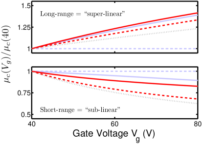
Figure 1: (Color online) Bilayer graphene mobility as a function of back-gate voltage $V_{g}$, normalized by the mobility at $V_{g}=40~{}{\rm V}$. Solid lines use bilayer graphene’s hyperbolic dispersion relation, while dashed lines are the parabolic approximation valid only for low carrier density. Upper panel – long-ranged Coulomb impurities. From bottom to top: over-screened (parabolic), RPA (parabolic), Thomas-Fermi (parabolic), over-screened (hyperbolic), Thomas-Fermi (hyperbolic). Lower panel: short-range (i.e. “delta-correlated” or “white noise”) impurities. From bottom to top: RPA (parabolic), Thomas-Fermi (parabolic), Thomas-Fermi (hyperbolic), unscreened (hyperbolic), unscreened (parabolic). See Ref. Das Sarma et al., 2010a for definitions of the different approximations.

Given a microscopic model for the disorder, one can compute both $\mu_{c}$ and $n_{\rm rms}$. Shown in Fig. 1 are results for bilayer graphene mobility assuming both short-range and Coulomb disorder with different approximations for the screening, and for both parabolic and hyperbolic dispersion relations. As seen from the figure, generically, Coulomb impurities show a super-linear dependence on carrier density while short-range scattereres are sub-linear. Similar to monolayer graphene,Adam et al. (2007); Jang et al. (2008); Ponomarenko et al. (2009) increasing the dielectric constant tends to decrease (increase) the scattering of electrons off long (short) range impurities, except in the over-screened and unscreened limits. All experiments to date find the mobility to be linear in gate voltage, so it is unclear what the dominant scattering mechanism in bilayer graphene is (see also discussion in Ref. Xiao et al., 2010). Further experiments along the lines of Refs. Jang et al., 2008; Ponomarenko et al., 2009 are needed.

In what follows we take $\mu_{c}$ and $n_{\rm rms}$ to be parameters of the theory that can be determined directly from experiments: $\mu_{c}$ can be obtained from low temperature transport measurements and $n_{\rm rms}$ from local probe measurements.Deshpande et al. (2009); Martin et al. (2008); Zhang et al. (2009); Miller et al. (2009) Lacking such microscopic measurements for the samples we compare with, we treat $n_{\rm rms}$ as a fitting parameter, while taking $\mu_{c}$ from experiment. As a consequence of this parameterization, the results reported here do not depend on the microscopic details of the impurity potential, provided this parameterization reasonably characterizes the properties of the impurity potential. Until more information about the important scattering centers is determined from experiment, all microscopic models will require a similar number of parameters such as the concentration of impurities $n_{\rm imp}$ and their typical distance $d$ from the graphene sheet. Further, the results will disagree with experiment unless the choices give a constant mobility.

A key assumption in this work is the applicability of Effective Medium Theory (EMT), which describes the bulk conductivity $\sigma_{\rm EMT}$ of an inhomogeneous medium by the integral equation Rossi et al. (2009)

$$\int dnP[n]\frac{\sigma(n)-\sigma_{\rm EMT}}{\sigma(n)+\sigma_{\rm EMT}}=0.$$ (3)

$P[n]$ is the probability distribution of the carrier density in the inhomogeneous medium – positive (negative) $n$ corresponds to (electrons) holes, and $\sigma(n)$ is the local conductivity of a small patch with a homogeneous carrier density $n$. Ignoring the denominator, Eq. 3 gives $\sigma_{\rm EMT}$ equal to the average conductivity. The denominator weights the integral to cancel the build-up of any internal electric fields. The EMT description has been shown to work well whenever the transport is semiclassical and quantum corrections and any additional resistance caused by the $p-n$ interfaces between the electron and hole puddles can be ignored.Rossi et al. (2009); Adam et al. (2009a); Fogler (2009) It is assumed that the band structure is not altered by the disorder, which is to be expected for the experimentally relevant disorder concentrations.Pershoguba et al. (2009) Since we are concerned with diffusive transport in the dirty limit, we expect that the EMT results hold for bilayer graphene.

III Results

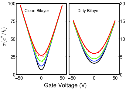
Figure 2: (Color online) Conductivity vs. gate voltage for clean and dirty graphene bilayers calculated from Eq. 3. Solid curves use the hyperbolic dispersion relation while dashed lines (only distinguishable at high temperature) show the parabolic approximation. Choice of parameters were based on experiments of Ref. Morozov et al., 2008 (clean) and Ref. Fuhrer, 2009 (dirty). Left panel: $\mu_{c}=6,750~{}{\rm cm}^{2}/{\rm Vs}$, $n_{\rm rms}=4\times 10^{11}~{}{\rm cm}^{-2}$ and (from bottom to top) T = 20 K, 100 K, 180 K and 260 K. Right panel: $\mu_{c}=1,100~{}{\rm cm}^{2}/{\rm Vs}$, $n_{\rm rms}=1.25\times 10^{12}~{}{\rm cm}^{-2}$ and (from bottom to top) T = 12 K, 105 K, 171 K and 290 K.

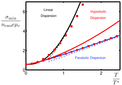
Figure 3: (Color online) Minimum conductivity as a function of temperature for linear dispersion (upper curve) and parabolic dispersion (lower curve) graphene. Dashed lines show the high temperature asymptotes $\sigma_{\rm min}\rightarrow\pi e\mu_{c}T^{2}/(3\hbar^{2}v_{\rm F}^{2})$ for linear and $\sigma_{\rm min}\rightarrow me\mu_{c}4\ln 2T/(\pi\hbar^{2})$ parabolic cases. Solid (red) line shows the hyperbolic result for $n_{\rm rms}=10^{12}{\rm cm}^{-2}$. Also shown is that the hyperbolic result extrapolates from the parabolic theory at large $\alpha=m^{2}v_{\rm F}^{2}/(\hbar^{2}\pi n_{\rm rms})$ becoming similar to the linear dispersion for small $\alpha$. (Red squares show results for $\alpha=100$ and red circles are for $\alpha=0.01$; here we ignore the contribution from higher bands).

To solve Eq. 3 we make the additional assumption that the distribution function $P[n,n_{g}]$ is Gaussian centered at $n_{g}$, (i.e. the field effect carrier density induced by the back gate that is proportional to $V_{g}$), with width $n_{\rm rms}$. (This assumption is justified both theoreticallyMorgan (1965); Stern (1974); Galitski et al. (2007); Adam et al. (2009b) and empiricallyDeshpande et al. (2009)). Our results are shown in Fig. 2, where as discussed earlier, the temperature dependence comes from the smearing of the Fermi surface.

At first glance, it is not obvious that the results for clean bilayer graphene (left panel of Fig. 2) and dirty bilayer graphene (right panel) are closely related. However, if we consider scaling the conductivity as ${\tilde{\sigma}_{\rm EMT}}=\sigma_{\rm EMT}/(n_{\rm rms}e\mu_{c})$, scaling temperature as $t=T/T^{*}$, where we define $k_{\rm B}T^{*}=E_{\rm F}(n=n_{\rm rms})$, and scaling carrier density as $z=n/n_{\rm rms}$, we find that for both the linear band dispersion $(n\gg n_{0})$ and the parabolic band dispersion $(n\ll n_{0})$, the scaled functions ${\tilde{\sigma}_{\rm EMT}}(z,t)$ each follow a universal curve. This is illustrated in Fig. 3 where we show the temperature dependence of the minimum conductivity. The results for the hyperbolic dispersion (which is the correct approximation at experimentally relevant carrier densities), depends on an additional parameter $\alpha=n_{0}/n_{\rm rms})$.kn: (b)

The scaling function for the hyperbolic dispersion extrapolates from the parabolic theory at large $\alpha$ becoming similar to the linear result for small $\alpha$. For the experimentally relevant regime $\alpha\approx 1$ the hyperbolic result depends only weakly on $\alpha$ and is indistinguishable from the parabolic result for $T\lesssim 0.5~{}T^{*}$.

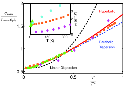
Figure 4: (Color online) Same results as in Fig. 3 showing comparison with experimental data from several groups. Inset shows the unscaled experimental data, while the main panel shows that the data collapses onto the theoretical curve with one scaling parameter ($n_{rms}$), where for each of these samples, we also use the value of mobility reported by the authors and obtained from a separate low temperature measurement. Green triangles show suspended bilayer data from Ref. Feldman et al., 2009 using $\mu_{c}=1.4~{}\mbox{\rm m}^{2}/\mbox{Vs}$ and $T^{*}=36~{}{\rm K}$. Orange squares (Ref. Fuhrer, 2009) and diamonds (Ref. Zhu et al., 2009) are bilayers on a SiO₂ substrate with $\mu_{c}=0.11~{}\mbox{\rm m}^{2}/\mbox{Vs}$, $T^{*}=530~{}{\rm K}$ and $\mu_{c}=0.045~{}\mbox{\rm m}^{2}/\mbox{Vs}$ and $T^{*}=290~{}{\rm K}$. Cyan circles show the four data points of Ref. Morozov et al., 2008, with $\mu_{c}=0.675~{}\mbox{\rm m}^{2}/\mbox{Vs}$, $T^{*}=80~{}{\rm K}$, which are off-scale in the main panel.

This analysis suggests that $\sigma_{\rm min}(T)/(e\mu_{c})$, which can be taken directly from experiment, is not a function of $\mu_{c}$, but only $n_{\rm rms}$. We take results from a set of experiments in very different regimes (see the inset of Fig. 4) and choose $n_{\rm rms}$ to fix the value of $\sigma_{\rm min}(T)/(n_{\rm rms}e\mu_{c})$ at $T=0$. Then using $k_{\rm B}T^{*}(n_{\rm rms})=E_{\rm F}(n_{\rm rms})$ to scale the temperature, all of the results lie on top of the theoretical curve computed using the hyperbolic dispersion, see Fig. 4. The theoretical curve with which they agree is distinct from similar curves calculated for a linear dispersion and for the purely parabolic dispersion at high $T/T^{*}$. We note that the scaling function is more complicated than a line. The calculation reproduces not only the initial slope as a function of temperature, but the crossover to higher temperature behavior. For the parabolic dispersion, which agrees at low temperatures, the conductivity extrapolates from $\sigma_{\rm min}(T\rightarrow 0)/(n_{\rm rms}e\mu_{c})\approx 3^{-1/2}$ at low temperature to $\sigma_{\rm min}(t\gg 1)/(n_{\rm rms}e\mu_{c})\approx(2\ln 2)t$ at high temperature, with a crossover temperature scale of $T\approx T^{*}/2$. In the future, it should be possible to further test this agreement by measuring $n_{\rm rms}$ experimentally. Deshpande et al. (2009); Martin et al. (2008); Zhang et al. (2009); Miller et al. (2009)

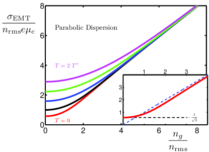
Figure 5: (Color online) Bilayer layer graphene conductivity as a function of temperature and carrier density for $T/T^{*}=0,0.5,1,1.5$, and $2$. Inset shows a close-up of the zero temperature minimum conductivity (which is the same for both monolayer and bilayer graphene). The dashed horizontal line shows the result for $\sigma_{\rm min}$, while the other dashed line is the high-density transport regime. The solid line (Eq. 4) captures the full crossover from the regime where the conductivity is dominated by the disorder induced carrier density fluctuations, to the semiclassical Boltzmann transport regime.

One feature of Fig. 2 and Fig. 4 is that for most of the experimentally relevant regime, the temperature dependence of the conductivity calculated using the parabolic approximation provides an adequate solution. This limit has been treated in contemporaneous work Das Sarma et al. (2010b); Lv and Wan (2010) treating this problem with different approximations and reaching similar conclusions. To better understand the emergence of a universal scaling form, we consider the conductivity for a parabolic band dispersion. Using the scaled variables defined above, we can manipulate Eq. (3) into the dimensionless form

$$\int_{0}^{\infty}dz\exp\left[-z^{2}/2\right]\cosh\left[z_{g}z\right]\frac{H[z,t]-{\bar{\sigma}}[z_{g},t]}{H[z,t]+{\bar{\sigma}}[z_{g},t]}=0,$$ (4)

where $z_{g}=n_{g}/n_{\rm rms}$ and we have written the local conductivity as $\sigma(n,T)=n_{\rm rms}e\mu_{c}H(z,t)$. Below we calculate the dimensionless function $H(z,t)$ assuming thermally activated carrier transport with constant $n_{\rm rms}$ and $\mu_{c}$ and explicitly show that it depends only on scaled variables $z=n/n_{\rm rms}$ and $t=T/T^{*}$. With the analytical results for $H(z,t)$ discussed below, this implicit equation can be solved either perturbatively or by numerical integration to give $\sigma_{\rm EMT}$. The results of this calculation are shown in Fig. 5.

To proceed, we calculate the function $H(z,t)$. For thermal activation of carriers, the chemical potential $\mu$ is determined by solving for $n_{g}=n_{e}-n_{h}$,Hwang and Das Sarma (2009) where

$$n_{e}(T) = \int_{0}^{\infty}dE~{}D(E)f(E,\mu,k_{\rm B}T),$$

$$n_{h}(T) = \int_{-\infty}^{0}dE~{}D(E)\left[1-f(E,\mu,k_{\rm B}T)\right],$$ (5)

where $f(E,\mu,k_{\rm B}T)$ is the Fermi-Dirac function and $k_{\rm B}$ is the Boltzmann constant. For $T=0$, only majority carriers are present, while for $T\rightarrow\infty$, activated carriers of both types are present in equal number. Within the parabolic approximation, we find $n_{e(h)}=n_{g}(T/T_{\rm F})\ln\left[1+\exp(\mp\mu/k_{\rm B}T)\right]$ and $\mu=E_{\rm F}$. Using $\sigma(n,T)=(n_{e}+n_{h})e\mu_{c}$, we obtain

$$H(z,t)=z+2t\ln\left[1+e^{-z/t}\right].$$ (6)

This demonstrates that Eq. 4 depends only on the scaled variables, guaranteeing that ${\tilde{\sigma}}_{\rm EMT}$ is a function only of $T/T^{*}$ and $n_{g}/n_{\rm rms}$ as shown in Fig. 5.

A similar analysis can be done for the hyperbolic dispersion. We find

$$H(z,t,\alpha)= \frac{z}{\xi+2}\left[4tg\ln[1+e^{-y/tg}]+2y\frac{}{}\right.$$ (7)

$$\mbox{}\left.+\frac{(tg\pi)^{2}\xi}{3}+\xi y^{2}\right],$$

where $g(z,\alpha)=T^{*}/T_{\rm F}$, $\xi(z,\alpha)=-1+\sqrt{1+z/\alpha}$, and the scaled chemical potential $y=\mu/E_{\rm F}$ is given by

$$y=\frac{1}{2}\left[2+\xi-2\xi(tg)^{2}({\rm Li}_{2}(-e^{-y/tg})-{\rm Li}_{2}(-e^{+y/tg}))\right],$$ (8)

where ${\rm Li}_{2}(z)=\int_{z}^{0}dt~{}t^{-1}\ln(1-t)$ is the dilogarithm function. Only for $\alpha\gg 1$ and $\alpha\ll 1$ does $H(z,t,\alpha)$ become independent of $\alpha=n_{0}/n_{\rm rms}$ giving the universal scaling forms for linear and parabolic dispersions, respectively.

IV Conclusion

In summary, we have developed an effective medium theory that captures the gate voltage and temperature dependence of the conductivity for bilayer graphene. The theory depends on two parameters: $n_{\rm rms}$ that sets the scale of the disorder, and $\mu_{c}$ the carrier mobility. These could be computed a priori by assuming a microscopic model for the disorder potential and its coupling to the carriers in graphene. Alternatively, one could use an empirical approach where one uses experimental data at $T=0$ to determine the parameters and use the theory to predict the temperature dependence.

Our main finding is that experimental data taken from various groups collapse onto our calculated scaling function where the disorder sets the scale of the temperature dependence of the conductivity. This further suggests that even some suspended bilayer samples are still the the diffusive (rather than ballistic) transport regime.