Creation of a Photonic Time-bin Qubit via Parametric Interaction of Photons in a Driven Resonant Medium

Abstract

A novel method of preparing a single photon in temporally-delocalized entangled modes is proposed and analyzed. We show that two single-photon pulses propagating in a driven nonabsorbing medium with different group velocities are temporally split under parametric interaction into well-separated pulses. As a consequence, the single-photon ”time-bin-entangled” states are generated with a programmable entanglement, which is easily controlled by driving field intensity. The experimental study of nonclassical features and nonlocality in generated states by means of balanced homodyne tomography is discussed.

I INTRODUCTION

Entanglement and nonlocal correlations, besides their fundamental importance in the modern interpretation of quantum phenomena ein ; bell , are the basic concepts for realization of quantum information procedures ben . The entanglement between matter and light states is an essential element of quantum repeaters breig , the intermediate memory nodes in quantum communication network aimed at preventing the photon attenuation over long distances. The two-photon entanglement is a crucial ingredient for quantum cryptography ekert ; tittel , quantum teleportation bouw ; furus ; marc , and entanglement swapping zuk ; pan , which have been successfully realized during the last decade by utilizing two approaches, one based on continuous quadrature variables and the other using the polarization variables of quantized electromagnetic field braun . An essential step has been recently made in this direction by implementing robust sources producing the pairs of photons which are entangled in well-separated temporal modes (time-bins) brend . It has been shown brend ; ried that this type of entanglement, in contrast to other ones, can be transferred over significantly large distances without appreciable losses, thus being much preferable for long-distance applications. From the fundamental viewpoint, of special interest is a single photon delocalized into two distinct spatial knill or temporal modes. In the last decade, the concept of single particle entanglement has been an object of intensive debates hardy ; peres ; green ; van . Although, there was some criticism in literature green concerning whether a single degree of freedom can be entangled with itself, it is now well recognized that a single photon state delocalized spatially or temporally in the two modes is entangled and nonlocal hardy ; peres ; van . Moreover, one-particle entangled qubit has been used to develop and further study of quantum cryptography jlee , quantum computing with linear optics knill or teleportation villas ; hlee ; giac . The robust criteria banas ; hill are now available for verification of entanglement and nonlocality of a correlated two-mode quantum state of light via testing the Bell’s inequality that has been recently realized experimentally babi ; zava by performing the homodyne detection of delocalized single-photon Fock states and reconstructing the corresponding Wigner function from homodyne data (see also lvov ).

Two approaches have been hitherto developed for preparation of a single-photon in two distinct temporal modes. In first one a time-bin qubit is created with use of linear optics by passing a short pulse from a spontaneous parametric down conversion (SPDC) source through Mach-Zehnder interferometer with different-length arms brend . The second approach is based on conditional measurement on quantum system of entangled signal-idler pairs generated via SPDC of two consecutive pump pulses in a nonlinear crystal, when a detection of one idler photon tightly projects the signal field into a single-photon state coherently delocalized over two temporal modes zava . However, the both methods are confronted with severe challenges. The main limitation is that the light emitted via SPDC has too broad linewidth ($\sim$ 10nm) and low spectral brightness to be able to excite atomic species. Additionally, due to short coherence time ($\sim$ femtosecond) the photon waveforms are not or hardly resolvable by existing photodetectors, as well as their coherence length is small for long distance quantum communication.

In this paper a novel method free from the above drawbacks is discussed for dynamical preparation of photonic time-bin qubit

$$\mid\psi\rangle=r_{1}\mid 1\rangle_{t}\mid 0\rangle_{t+\tau}+r_{2}\mid 0\rangle_{t}\mid 1\rangle_{t+\tau}$$ (1)

where $\mid 0\rangle_{t}$ and $\mid 1\rangle_{t}$ denote Fock states with zero and one photon, respectively, at the time $t$ and $\mid r_{1}\mid^{2}+\mid r_{2}\mid^{2}=1$. The basic idea is to create a parametric interaction between two single-photon pulses, which

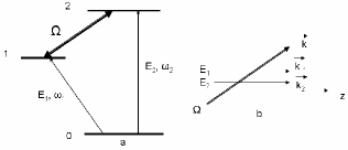
Figure 1: (a) Level scheme of atoms interacting with quantum fields $E_{1,2}$ and classical rf driving field of Rabi frequency $\Omega.$ (b) Geometry of fields propagation.

propagate in a resonantly driven medium without absorption and at low, but different, group velocities. Then, due to the cyclic parametric conversion of the fields and the group delay, each pulse experiences a temporal splitting into well-separated subpulses. Moreover, since the process is completely coherent, at the output of the medium the time-delocalized and entangled single-photon state is formed. One obvious limitation of this resonant process is that it is effective in a relatively narrow frequency range associated with specific atoms. We note, however, that recently a source of narrow-bandwidth, frequency tunable single photons with properties allowing exciting the narrow atomic resonances has been created chou ; eis . Thus, our mechanism is a robust source for temporally entangled narrow-bandwidth single-photons. Another important advantage is a generation in a simple manner of any desired entanglement by controlling the driving field intensity. In section II we describe a three-level model parametric interaction between two quantum fields propagating in a driven medium under the conditions of electromagnetically induced transparency (EIT). Then, in realistic approximations, we obtain an analytical solution for the field operators and calculate the output intensities of the fields showing the splitting of an initial single-photon pulse into two well separated temporal modes. In section III we analyze the entanglement characterizing our single-photon state by employing the Bell’s inequality proposed by Banaszek and Wodkiewicz banas and show an unambiguous correspondence of this inequality violation to the degree of two-mode single-photon entanglement. Finally, in section IV we summarize our conclusions.

II THREE-LEVEL MODEL OF PHOTON PARAMETRIC INTERACTION

We consider an ensemble of cold atoms with level configuration depicted in Fig.1. Two quantum fields

$$E_{1,2}(z,t)=\sqrt{\frac{\hbar\omega_{1,2}}{2{\varepsilon}_{0}V}}\hat{\mathcal{E}}_{1,2}(z,t)\exp[i(k_{1,2}z-\omega_{1,2}t)]+h.c.$$

co-propagate along the $z$ axis and interact with the atoms on the transitions $0\rightarrow 1$ and $0\rightarrow 2$, respectively, while the electric-dipole forbidden transition $1\rightarrow 2$ is driven by a classical and constant radio-frequency (rf) field with real Rabi frequency $\Omega$ inducing a magnetic dipole or an electric quadrupole transition between the two upper levels, and $V$ is the quantization volume taken to be equal to interaction volume. The electric fields are expressed in terms of the operators $\hat{\mathcal{E}}_{i}(z,t)$ obeying the commutation relations (see Appendix A)

$$[\hat{\mathcal{E}}_{i}(z,t),\hat{\mathcal{E}}_{j}^{+}(z,t^{\prime})]=\frac{L}{c}\delta_{ij}\delta(t-t^{\prime})$$ (2)

where $L$ is the length of the medium. We describe the latter using atomic operators $\hat{\sigma}_{\alpha\beta}(z,t)$ $=\frac{1}{N_{z}}\underset{i=1}{\overset{N_{z}}{\sum}}\mid\alpha$ $\rangle_{i}\langle\beta\mid$ averaged over the volume containing many atoms $N_{z}=\frac{N}{L}dz\gg 1$ around position $z$, where $N$ is the total number of atoms. In the rotating wave picture the interaction Hamiltonian is given by

$$H=-\hbar\frac{N}{L}\int\limits_{0}^{L}dz[g_{1}\hat{\mathcal{E}}_{1}\hat{\sigma}_{10}e^{ik_{1}z}+g_{2}\hat{\mathcal{E}}_{2}\hat{\sigma}_{20}e^{ik_{2}z}+\Omega\hat{\sigma}_{21}e^{ik_{\parallel}z}$$

$$+h.c.]$$ (3)

Here $k_{\parallel}=\vec{k}_{d}\hat{e}_{z}$  is the projection of the wave-vector of the driving field on the $z$ axis, $g_{\alpha}=\mu_{\alpha 0}\sqrt{{\omega_{i}}/(2{\hbar\varepsilon}_{0}V})$ is the atom-field coupling constants with $\mu_{\alpha\beta}$ being the dipole matrix element of the atomic transition $\alpha\rightarrow\beta$. For simplicity, we discuss the case of exactly resonant interaction with all fields and, therefore, put in Eq.(3) the frequency detunings equal to zero, neglecting so the Doppler broadening, which in a cold atomic sample is smaller than all relaxation rates. Then, using the slowly varying envelope approximation, the propagation equations for the quantum field operators take the form:

$$\left(\frac{\partial}{\partial z}+\frac{1}{c}\frac{\partial}{\partial t}\right)\hat{\mathcal{E}}_{1}(z,t)=ig_{1}\frac{N}{c}\hat{\sigma}_{01}e^{-ik_{1}z}+\hat{F}_{1}$$ (4)

$$\left(\frac{\partial}{\partial z}+\frac{1}{c}\frac{\partial}{\partial t}\right)\hat{\mathcal{E}}_{2}(z,t)=ig_{2}\frac{N}{c}\hat{\sigma}_{02}e^{-ik_{2}z}+\hat{F}_{2}$$ (5)

where $\hat{F}_{i}(z,t)$ are the commutator preserving Langevin operators, whose explicit form is given below.

In the weak-field (single-photon) limit, the equations for atomic coherences $\hat{\rho}_{0i}=\hat{\sigma}_{0i}e^{-ik_{i}z},\ \ i=1,2~{}\ \ \$and$\ \ \ \ \ \hat{\rho}_{12}=\hat{\sigma}_{12}e^{-i(k_{2}-k_{1})z}\$ are treated perturbatively in $\hat{\mathcal{E}}_{1,2}$. In the first order only $\langle\hat{\sigma}_{00}\rangle\simeq 1$ is different from zero and for these equations we obtain:

$$\frac{\partial}{\partial t}\hat{\rho}_{01}=-\Gamma_{1}\hat{\rho}_{01}+ig_{1}\hat{\mathcal{E}}_{1}\hat{\sigma}_{00}+i\Omega\hat{\rho}_{02}e^{i\bigtriangleup kz}-ig_{2}\hat{\mathcal{E}}_{2}\hat{\rho}_{21}$$ (6)

$$\frac{\partial}{\partial t}\hat{\rho}_{02}=-\Gamma_{2}\hat{\rho}_{02}+ig_{2}\hat{\mathcal{E}}_{2}\hat{\sigma}_{00}+i\Omega\hat{\rho}_{01}e^{-i\bigtriangleup kz}-ig_{1}\hat{\mathcal{E}}_{1}\hat{\rho}_{12}$$ (7)

$$\frac{\partial}{\partial t}\hat{\rho}_{12}=-\Gamma_{12}\hat{\rho}_{12}-ig_{1}\hat{\mathcal{E}}_{1}^{\ast}\hat{\rho}_{02}+ig_{2}\hat{\mathcal{E}}_{2}\hat{\rho}_{10}$$ (8)

Here $\Delta k=k_{2}-k_{1}-k_{\parallel}$ is the wave-vector mismatch and $\Gamma_{1,2}$ and $\Gamma_{12}$ are the transverse relaxation rates involving, apart from natural decay rates $\gamma_{1,2}$ of the excited states 1 and 2, the dephasing rates in corresponding transitions. The latter are caused by atomic collisions and escape of atoms from the laser beam. However, in the ensemble of cold atoms the both effects are negligibly small compared to $\gamma_{1,2}$, so that $\Gamma_{1,2}$=$\gamma_{1,2}/2$ and $\Gamma_{12}$=$(\gamma_{1}+\gamma_{2})/2$.

Further, we assume that the phase-matching condition $\Delta k=0$ is fulfilled in the medium. Then, the solution to Eqs.(6-8) to the first order in $\hat{\mathcal{E}}_{1,2}$ is readily found to be

$$\hat{\rho}_{01}=i\frac{\Gamma}{D}g_{1}\hat{\mathcal{E}}_{1}+i\frac{\Omega^{2}-\Gamma^{2}}{D^{2}}g_{1}\frac{\partial}{\partial t}\hat{\mathcal{E}}_{1}-\frac{\Omega}{D}g_{2}\hat{\mathcal{E}}_{2}+\frac{2\Gamma\Omega}{D^{2}}g_{2}\frac{\partial}{\partial t}\hat{\mathcal{E}}_{2},$$ (9)

$$\hat{\rho}_{02}=\hat{\rho}_{01}(1\leftrightarrow 2),\ \ \ \text{ }D=\Omega^{2}+\Gamma^{2}.$$ (10)

where, for simplicity, the optical decay rates are taken to be the same: $\Gamma_{1}=\Gamma_{2}=\Gamma$. The first terms in right hand side (RHS) of Eqs.(9,10) are responsible for linear absorption of quantum fields and define the field absorption coefficients $\kappa_{i}={g_{i}^{2}\Gamma N}/{c\Omega^{2}}$ upon substituting these expressions into Eqs.(4,5). Here the condition of electromagnetically induced transparency (EIT, refs. harris ; mfleis ) $\Omega\gg\Gamma_{1,2}$ is assumed to be satisfied for both transitions coupled to the weak-fields. Note that the three-level configurations 0-2-1 and 0-1-2 form the $\Lambda$- and ladder EIT-systems, respectively, with the same decoherence time $\Gamma^{-1}$ banac . The second terms in RHS of Eqs.(9,10) represent the dispersion contribution to the group velocities of the pulses, while the two rest terms describe the parametric interaction between the fields. We require that the photon absorption be strongly reduced by imposing the condition $\kappa_{i}L\ll 1.$ Another limitation follows from $\Delta\omega_{EIT}T\geq 1$ indicating that the initial spectrum of quantum fields is contained within the EIT window $\Delta\omega_{EIT}={\Omega^{2}}/({\Gamma\sqrt{\alpha}})$ fleis , where $T$ is a duration of weak-field pulses, $\alpha=\mathcal{N}\sigma L$ is the optical depth, $\sigma=\frac{3}{4\pi}\lambda^{2}$ is the resonant absorption cross-section, and $\mathcal{N}$ is the atomic number density. Finally, the length of the pulses has to fit the length of the medium: $Tv_{i}<L$ with $v_{i}={c\Omega^{2}}/{g_{i}^{2}N}$ being the group velocity of the $i$-th field. Taking into account that $\kappa_{i}L\sim\Gamma^{2}\alpha/\Omega^{2}$, this set of limitations yields

$$\frac{\Omega^{2}}{\Gamma^{2}}>>\alpha\text{ \ \ \ \ and \ }\frac{1}{\sqrt{\alpha}}\ll\frac{Tv_{i}}{{}_{L}}<1\text{\ \ \ }$$ (11)

It is worth noting that upon satisfying the conditions (11), the dominant contribution to the parametric coupling between the photons is the third term in RHS of Eq.(9,10), because in this case the last term becomes strongly suppressed by the factor $\Omega^{2}T/\Gamma>>1.$

It is useful at this point to consider numerical estimations. The sample is chosen to be ${}^{87}Rb$ vapor with the ground state $5S_{1/2}(F_{g}=2)$ and exited states $5P_{3/2}(F_{e}=2)$, $5P_{3/2}(F_{e}=3)$ being the atomic states $0$ and $1,2$ in Fig.1, respectively. Using the following parameters - light wavelength $\lambda\simeq 0.8\mu$m, $\Gamma=2\pi\times 3$ MHz, atomic density $\mathcal{N}\sim 10^{12}$cm^-3 in a trap  of length $L\sim 100$ $\mu$m, $\Omega\sim 10\Gamma,$ and the input pulse duration $T\simeq$ 2$\div$3ns, we find $\alpha\simeq 16,$ $v_{2}\sim 10^{4}m/s$, $v_{1}\sim 0.3v_{2},$ and $\kappa_{i}L\leqslant 0.1$. All of the parameters we use in our calculations appear to be within experimental reach, including the initial single-photon wave packets with a duration of several nanoseconds satisfying the narrow-line limitation discussed above.

The noise operators $F_{1,2}$ in Eqs.(4,5) have the properties scully

$$\langle F_{i}(z,t)\rangle=\langle F_{i}(z,t)F_{i}(z,t^{\prime})\rangle=\langle F_{i}(z,t)F_{j}(z,t^{\prime})\rangle=0$$

$$\langle F_{i}(z,t)F_{j}^{+}(z,t^{\prime})\rangle=2\frac{\kappa_{i}}{c}\delta_{ij}\delta(t-t^{\prime})$$

showing that in the absence of photon losses the noise operators $\hat{F}_{i}$ give no contribution. Then, in this limit the simple propagation equations for the field operators are obtained:

$$\left(\frac{\partial}{\partial z}+\frac{1}{v_{1}}\frac{\partial}{\partial t}\right)\hat{\mathcal{E}}_{1}(z,t)=-i\beta\hat{\mathcal{E}}_{2}$$ (12)

$$\left(\frac{\partial}{\partial z}+\frac{1}{v_{2}}\frac{\partial}{\partial t}\right)\hat{\mathcal{E}}_{2}(z,t)=-i\beta\hat{\mathcal{E}}_{1}$$ (13)

where $\beta={g_{1}g_{2}N/c\Omega}$ is the parametric coupling constant. In Appendix A we show that these equations preserve the commutation relations (2). Note that for the parameters above, the parametric interaction between the photons is sufficiently strong: $\beta L\sim 3$.

The formal solution of Eqs.(12,13) for the field operators in the region $0\leqslant z\leqslant L$ is written as

$$\hat{\mathcal{E}}_{i}(z,t)=\hat{\mathcal{E}}_{i}(0,\ t-z/v_{i})+\int\limits_{0}^{z}dx\{\hat{\mathcal{E}}_{i}(0,\ t-z/v_{j}-\frac{\Delta v_{ji}}{v_{i}v_{j}}x)$$

$$\times\frac{\partial J_{0}(\psi)}{\partial z}-i\beta\ \hat{\mathcal{E}}_{j}(0,\ t-z/v_{i}-\frac{\Delta v_{ij}}{v_{i}v_{j}}x)\ J_{0}(\psi)\},\$$ (14)

where $i,j=1,2$  and $j\neq i.$ The Bessel function $\ J_{0}(\psi)$ depends on $z$ via $\psi=2\beta\sqrt{x(z-x)}$ , $\Delta v_{ij}=v_{i}-v_{j}$ is the difference of group velocities.

We are interested in the evolution of the input state $\mid\psi_{in}\rangle=\mid 1_{1}\rangle\otimes\mid 0_{2}\rangle$ consisting of a single-photon wave packet at $\omega_{1}$ frequency, while $\omega_{2}$ field is in the vacuum state. The similar results are clearly obtained in the case of one input photon at $\omega_{2}$ frequency. We assume that initially the $\omega_{1}$ pulse is localized around $z=0$ with a given temporal profile $f_{1}(t):$

$$\langle 0\mid\hat{\mathcal{E}}_{1}(0,t)\mid\psi_{in}\rangle=\langle 0\mid\hat{\mathcal{E}}_{1}(0,t)\mid 1_{1}\rangle=f_{1}(t)$$ (15)

where $f_{1}(t)$ is normalized as $\frac{c}{L}\int\mid f_{1}(t)\mid^{2}dt=1$. In free space, $\hat{\mathcal{E}}_{1}(z,t)=\hat{\mathcal{E}}_{1}(0,t-z/c)$ and we have

$$\langle 0\mid\hat{\mathcal{E}}_{1}(0,t-z/c)\mid 1_{1}\rangle=f_{1}(t-z/c).$$ (16)

The intensities of the fields at any distance in the region $0\leqslant z\leqslant L$ are given by

$$\langle I_{i}(z,t)\rangle=\mid\langle 0\mid\hat{\mathcal{E}}_{i}(z,t)\mid\psi_{in}\rangle\mid^{2}$$ (17)

Using Eqs.(14-16) and recalling that $\langle 0\mid\hat{\mathcal{E}}_{2}(0,t)\mid\psi_{in}\rangle=0$, we calculate $\langle I_{i}\rangle$ numerically and show in Fig.2 the output pulses at $z=L$ for the three values of $\Omega$ and for Gaussian input (at $z=0$) pulse $f_{1}(t)=C\exp[-2t^{2}/T^{2}]$, where $C$ is some normalization constant. For one-photon initial state, as is the case here, one can clearly see that the second field is not practically generated, thus demonstrating that our scheme enables to prepare a single-photon in a pure temporally-delocalized state with an efficiency $\sim 100\%.$ Moreover, depending on the driving field intensity, a different degree of initial pulse splitting is attainable. It is easy to check that the total number of photons which is determined by the areas of the corresponding peaks is conserved upon propagation through the medium. To show this we introduce the dimensionless operators for numbers of photons that pass each point on z axis over the whole of time

$$\hat{n}_{i}(z)=\frac{c}{L}\int dt\hat{\mathcal{E}}_{i}^{+}(z,t)\hat{\mathcal{E}}_{i}(z,t)$$ (18)

With taking into account that $\langle 0\mid\hat{\mathcal{E}}_{i}(z,t\rightarrow\pm\infty)\mid\psi_{in}\rangle=0$, the conservation low for mean photon numbers results from Eqs.(12) and (13)

$$\frac{\partial}{\partial z}(n_{1}(z)+n_{2}(z))=0$$ (19)

Figure 2: Temporal shapes of quantum fields ($t$ is given in units of input pulse duration $T$) at the output of the medium $z=L$ for three values of $\Omega$. In these figures, solid curves represent the $\omega_{1}$ pulses, dashed curves show the $\omega_{2}$ field generated in the medium, and dotted lines display the initial Gaussian pulse at $\omega_{1}$ frequency with $T=2$ns propagating in the medium in the absence of parametric interaction $\beta=0.$ For the rest of parameters see the text.

where $n_{i}(z)=\langle\psi_{in}\mid\hat{n}_{i}(z)\mid\psi_{in}\rangle$. Since in our case $n_{2}(0)=0$ and $n_{2}(L)$ is negligibly small, we have $n_{1}(L)\simeq n_{1}(0)=1$. Thus, in the considered scheme we are able to preserve the output $\omega_{1}$-field in a single-photon state while modulating its amplitude to get a desirable spatio-temporal distribution. Further, only two well-separated output temporal modes at $\omega_{1}$ frequency are produced. To understand the physics of this splitting, let us discuss the structure of solution (14) for $\hat{\mathcal{E}}_{i}(z,t)$ in detail. The first term in this equation represents the $\omega_{1}$-pulse in the absence of $\omega_{2}$ generation. In such a case, the group velocity of the pulse is slowed down to $v_{1}<<c$ under the conditions of EIT realized via ladder system 0-1-2. However, the input $\omega_{1}$ photon can also be converted to one photon of the $\omega_{2}$ field which is emitted on the dipole-allowed transition $2\rightarrow 0$ and propagates in the medium at a group velocity $v_{2}<<c$ established under EIT in the $\Lambda$- scheme 0-2-1. In its turn, the $\omega_{2}$ photon is transformed back into $\omega_{1}$ photon, which precedes the signal $\omega_{1}$ photon owing to $v_{2}>v_{1}$. This process is described by the second term in Eq.(14). The last term in this equation corresponds to generation of an $\omega_{1}$ photon by an input $\omega_{2}$ photon and gives no contribution in our case. An important point here is that an atom, being excited to the upper state 2 upon absorbing the initial $\omega_{1}$ photon and one photon of the drive field, can return back to the ground state in two ways: 1) by emitting one photon of drive field and an $\omega_{1}$ photon and 2) by emitting an $\omega_{2}$ photon on the transition $2\rightarrow 0$. The competition between the two processes evidently leads to a destructive interference between the modes propagating in the $\omega_{1}$ channel with different group velocities and ultimately gives rise to the pulse temporal splitting. In Appendix B we show that, indeed, the contributions of the two processes into $\omega_{1}$ photon wavefunction are of opposite signs. The separation of $\omega_{1}$ temporal modes depends clearly on the relative velocity of quantum fields, the larger the ratio $v_{2}/v_{1}$, the larger the group delay and the larger the separation of the two output $\omega_{1}$ pulses. On the contrary, in the limit of equal group velocities $v_{2}=v_{1}=v$ the propagating pulses experience no splitting, as it follows from Eqs.(14), which in this case are reduced to

$$\hat{\mathcal{E}}_{i}(z,t)=\hat{\mathcal{E}}_{i}(0,\tau)cos(\beta z)-i\hat{\mathcal{E}}_{j}(0,\tau)sin(\beta z)$$ (20)

where $\tau=t-z/v$, $j\neq i.$

We finish this consideration with a short remark about the dynamics of frequency conversion from $\omega_{1}$ to $\omega_{2}$ and back to $\omega_{1}$ in dependence on the travelled distance. For equal group velocities $v_{1}=v_{2}$, a simplest result follows from Eq.(20) with $\langle 0\mid\hat{\mathcal{E}}_{2}(0,t)\mid\psi_{in}\rangle=0$. It is seen that the complete conversion of the input $\omega_{1}$ photon to one photon of the $\omega_{2}$ field occurs at the distance $z_{max}(v_{1}=v_{2})=\pi/(2\beta)$, which is proportional to $\Omega$ and thus exhibits the square-root dependence on the drive field intensity. An essentially different picture is observed for $v_{1}\neq v_{2}$. In this case the efficient frequency conversion from $\omega_{1}$ to $\omega_{2}$ takes place up to a distance, where the time delay between the signal $\omega_{1}$ and parametrically generated $\omega_{2}$ pulses becomes comparable to the pulse duration $T$. The numerical calculations show that, for the parameters above, this happens roughly at $z_{max}(v_{1}\neq v_{2})\simeq(v_{2}-v_{1})T\sim 20\mu$m. At this point, the $\omega_{2}$ field reaches its maximal value with conversion efficiency $\sim$ 0.13. For $z>z_{max}(v_{1}\neq v_{2})$ the two pulses are no longer overlapped in time, and the $\omega_{2}$ pulse is transformed to the fast $\omega_{1}$ pulse almost completely. Only a tiny part on the leading edge of the $\omega_{2}$ pulse leaves the medium with the group velocity $v_{2}$. With further propagation in the medium, the energy is merely pumped from the slow $\omega_{1}$ pulse to the fast one, while the $\omega_{2}$ field remains negligibly small. This occurs as long as the fast $\omega_{1}$ pulse becomes sufficiently strong in order to generate a new $\omega_{2}$ pulse. According to our analysis, the corresponding distance is approximately 130$\mu$m showing that in a sufficiently large interval of propagation lengths only the $\omega_{1}$ field is present in the medium in the form of two well separated temporal modes. This result provides a wide choice of the length of atomic sample that is important for further applications of the proposed mechanism.

It must be noted that the considered system is capable of fully entangling two single-photon pulses at different frequencies $\omega_{1}$ and $\omega_{2}$ in the case of input state $\mid\psi_{in}$ $\rangle=$ $\mid 1_{1}$ $\rangle\otimes\mid 1_{2}$ $\rangle$. The study of this problem is, however, beyond the scope of the present paper and its results will be published elsewhere. Here we note only that in this case two time-bin qubits at $\omega_{1}$ and $\omega_{2}$ are generated, being at the same time strongly correlated with each other. This correlation is clearly seen from the particular result of Eq.(20).

III NONLOCALITY IN GENERATED STATE: ANALYSIS OF BELL’S INEQUALITY

Now we discuss whether nonlocal correlations arise between the two generated temporal modes of a single $\omega_{1}$-photon and how they can be verified experimentally. We first note that the entanglement is not apparent in the single-photon wavefunction $\Phi_{1}(z,t)$, which is represented as a sum (see Eq.(B3)), rather than mixture product of two orthogonal mode functions $\Phi_{1}^{F}(z,t)$ and $\Phi_{1}^{S}(z,t)$. This does not mean, however, that the entanglement is absent in the photon state. It can appear in second quantization formalism, where the solution Eqs.(14) for the field operators has been found. The point is what representation of Fock space has to be chosen to make this effect visible, since, as it has been shown in pawl , the entanglement with vacuum and nonlocality in a single-photon state is not a property of the Fock space in general, but appears if a specific irreducible representation is chosen, although the same physics follows from all Fock representations in the sense that the experimental test of entanglement and nonlocality is performed by mapping the quantum field state into the state of the matter (single trapped atoms or ions, atomic ensembles, quantum dots, etc.) and the results of such measurements are the same independent of the representation. Below we describe the output $\omega_{1}$-photon state in terms of quantized temporal modes and choose the relevant representation for the field quantization.

Using the definitions of photon number operators Eq.(18) and wavefunction Eq.(B1), we obtain the $\omega_{1}$ single-photon output state as

$$\mid 1_{1}\rangle_{z=L}=\frac{c}{L}\int dt\Phi_{1}(L,t)\hat{\mathcal{E}}_{1}^{+}(L,t)\mid 0\rangle$$ (21)

Normalization requires that

$$\frac{c}{L}\int dt\mid\Phi_{1}(L,t)\mid^{2}=1$$

This condition, the left hand side of which coincides evidently with the mean photon number $n_{1}(L)$, manifests along with $n_{1}(0)=\frac{c}{L}\int dt\mid f_{1}(t)\mid^{2}=1$ the photon number conservation law. Remind that for intermediate values of $z$ ($0<z<L$) $n_{2}(z)$ is no longer zero and hence $n_{1}(z)<1$. At these distances the incoming $\omega_{1}$ field is converted, completely or partially, into $\omega_{2}$ optical mode that enables frequency conversion and redistribution of quantum information between different quantum fields. This mechanism will be discussed elsewhere.

Let us rewrite the Eq.(21) in the form

$$\mid 1_{1}\rangle_{z=L}=\frac{c}{L}\int dt(\Phi_{1}^{F}(L,t)+\Phi_{1}^{S}(L,t))\hat{\mathcal{E}}_{1}^{+}(L,t)\mid 0\rangle$$ (22)

and introduce the operators of creation of single-photon wave packets associated with orthogonal set of mode functions $\Phi_{1}^{i}(L,t)$ blow , where $i$ labels the members of the denumerably infinite set. For $i=F,S$ these operators are given by

$$\hat{c}_{F,S}^{+}=N_{F,S}^{1/2}\int dt\Phi_{1}^{F,S}(L,t)\hat{\mathcal{E}}_{1}^{+}(L,t)$$ (23)

with the normalization constants

$$N_{i}=\frac{c}{L}(\int dt\mid\Phi_{1}^{i}(L,t)\mid^{2})^{-1}$$ (24)

These operators create the single-photon states in the usual way by operation on the vacuum state $\mid 0\rangle$

$$\hat{c}_{i}^{+}\mid 0\rangle=\mid 1_{1}\rangle_{i}$$ (25)

and have the standard boson commutation relations

$$[\hat{c}_{i},\hat{c}_{j}^{+}]=\delta_{ij}$$ (26)

Note that this definition of quantum temporal modes is only useful, if one can perform the local measurements on these modes such that they are spacelike separated. That is why the requirement for the modes be well separated is important. Now, for the algebra (26) we choose the representation of infinite product of all vacua

$$\mid 0\rangle=\prod_{i}\mid 0\rangle_{i}=\mid 0\rangle_{F}\mid 0\rangle_{S}\prod_{i\neq F,S}{\mid 0\rangle_{i}}.$$ (27)

However, since in our problem we deal with two modes, while the other modes are not occupied by the photons and, hence, are not taken into account during the measurements, the vacuum may be reduced to $\mid 0\rangle=\mid 0\rangle_{F}\mid 0\rangle_{S}$. Then the single-photon state (22) can be written as

$$\mid 1_{1}\rangle_{z=L}=r_{1}\hat{c}_{F}^{+}\mid 0\rangle_{F}\mid 0\rangle_{S}+r_{2}\mid 0\rangle_{F}\hat{c}_{S}^{+}\mid 0\rangle_{S}$$

$$=r_{1}\mid 1\rangle_{F}\mid 0\rangle_{S}+r_{2}\mid 0\rangle_{F}\mid 1\rangle_{S}$$ (28)

which is just the state (1) with $r_{1,2}=\sqrt{\frac{c}{L}\int dt\mid\Phi_{1}^{F,S}(L,t)\mid^{2}}$. The remarkable property of chosen representation (27) is that in this case the entanglement in the single-photon state is entirely converted into nonlocal entanglement between the atoms pawl and, hence, the entanglement in the field state reproduces adequately the expected results of any measurement one may perform on atomic systems. The amount of entanglement in the state (28) is simply

$$E=-[r_{1}^{2}\log_{2}r_{1}^{2}+(1-r_{1}^{2})\log_{2}(1-r_{1}^{2})]$$ (29)

calculated as $E=-Tr_{S}[\rho\log_{2}\rho]$ with $\rho=Tr_{F}\mid 1_{1}\rangle\langle 1_{1}\mid$. It is easy to check that $E$ is maximal $E_{max}=1$ for $r_{1}=\frac{1}{\sqrt{2}}$.

Now we pass to discussion of nonlocal correlations in the state (28). Note that the single-photon states are completely described by their Wigner function, whose remarkable property is that it takes negative values around the origin of phase space for the complex field amplitude. The negativity of the Wigner function is the ultimate signature of non-classical nature of these states. Besides, the nonlocality of quantum correlations in single-photon qubit is directly evident from the violation of Bell’s inequality formulated for two-mode Wigner function. Specifically, we will employ the criterion proposed by Banaszek and Wodkiewicz banas allowing a Bell test with high levels of violation. The ability of this approach has recently been demonstrated in the case of SPDC temporally entangled single photon zava . As has been shown in Ref.banas , the local theories impose the bound

$$-2\leqslant{\mathcal{B}}\leqslant 2$$ (30)

where the combination ${\mathcal{B}}$ has the form:

$${\mathcal{B}}=\frac{\pi^{2}}{4}[W(0,0)+W(\alpha_{1},0)+W(0,\alpha_{2})-W(\alpha_{1},\alpha_{2})]$$

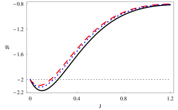
Figure 3: (color online) Plot of the combination ${\mathcal{B}(J)}$ (Eq.(32)) for three values of $r_{1}$: 0.4 (dashed); $1/\sqrt{2}$ (solid) and 0.9 (dotted) corresponding to three values of $\Omega$ in Fig.2. (from top to bottom).

Here $W(\alpha_{1},\alpha_{2})$ is the Wigner function of two temporal modes calculated for complex amplitudes $\alpha_{i}=x_{i}+iy_{i}$ with $x_{i}$ and $y_{i},i=1,2,$ being the quadratures of the $i$-th mode. The Wigner function for the state (28) is obtained to be:

$$W(\alpha_{1},\alpha_{2})=\frac{4}{\pi^{2}}[2\mid r_{1}\alpha_{1}+r_{2}\alpha_{2}\mid^{2}-1]e^{-2\mid\alpha_{1}\mid^{2}-2\mid\alpha_{2}\mid^{2}}$$ (31)

which is always negative $W(0,0)<0$ independent of $r_{1}$ and $r_{2}$. The amplitudes $r_{1}$ and $r_{2}$ depend on the driving field intensity and are calculated numerically.

Then the strongest violation of inequality (30) is achieved when $\alpha=\alpha_{1}=\alpha_{2}$, for which case the combination ${\mathcal{B}}$ takes the form:

$${\mathcal{B}}=-1+(4J-2)e^{-2J}-[4J(r_{1}+\sqrt{1-r_{1}^{2}})^{2}-1]e^{-4J}$$ (32)

where $J=\alpha^{2}$. Its behavior is plotted in Fig.3 as a function of $J$ for the values of $r_{1}$ corresponding to three output states of $\omega_{1}$ photon depicted in Fig.2. It is evident that the maximal violation, which is about ten percent (2.2 compared to a classical maximum of 2), is obtained at $\alpha=0.3$ for $r_{1}=1/\sqrt{2}$, i.e. when the output temporal modes are produced with equal probabilities. Similar to the previous works zava ; lvov , the Wigner function (22) can be experimentally reconstructed from the data of balanced homodyne detection, when the $\omega_{1}$ signals at the detectors are measured at two different times matched to the time separation between two output pulses obtained in Fig.2. However, a rigorous experimental demonstration of maximal violation is attainable in a loophole-free Bell test, when both locality and detection loopholes are closed in a single experiment loop . The locality-loophole can be easily avoided, if the homodyne detection of two co-propagating temporal modes is performed by one-photon detectors as fast as the two simultaneous measurements on each of the modes are separated by a spacelike interval. This may easily be achieved within our model, because the time separation between the two temporal modes amounts to several nanoseconds. To eliminate second, detection-efficiency loophole, we follow the works zava , although in these papers SPDC in nonlinear crystal has been used for generation of time-bin qubit. To satisfy the Banaszek-Wodkiewicz criterion one has to prepare pure single-photon state or the ”vacuum-cleaned” Wigner function. To this end the different methods have been applied in zava leading to the same result and showing a strict violation of Bell’s inequality in accordance with theoretical expectations.

IV CONCLUSIONS

In conclusion, we have demonstrated the possibility for dynamic preparation of a single photon in distinct temporal modes, employing strong parametric interaction between two slow single-photon pulses and their group delay. Disregarding the photon losses, we have found the solution of propagation equations for the quantum field operators depending on the propagation distance in terms of the Bessel function. Although the losses result in a decay of the field amplitudes, they do not prevent the temporal splitting of quantum pulses. Moreover, since the two well separated $\omega_{1}$ pulses undergo the same losses, the entanglement between them is almost insensitive to losses and easier to purify, so that the proposed scheme can be regarded as a robust source of narrow-bandwidth single-photon qubits. We have shown the ability of our scheme to achieve an arbitrary entanglement between the $\omega_{1}$ temporal modes by adjusting the driving field intensity, while the separation between the time bins can be controlled by using the different atomic-level configurations to obtain the different group velocities of quantum fields. Subsequent papers will discuss a possibility for transferring and distributing quantum information between optical modes of different frequencies $\omega_{1}$ and $\omega_{2}$ in a loss and decoherence-free fashion, as well as the more complicated case of two input single-photon pulses will be analyzed and the results of detail numerical simulations will be presented.

This work was supported by the ISTC Grant No.A-1095 and INTAS Project Ref.Nr 06-1000017-9234.

APPENDIX A: COMMUTATION RELATIONS FOR FIELD OPERATORS

In this Appendix we derive the commutation relations Eq.(1) for traveling-wave electric field operators. In free space $z\leq 0$, the field operators are given by $\hat{\mathcal{E}}_{i}(z,t)=\underset{n=0}{\overset{\infty}{\sum}}a_{i,n}e^{-i\omega_{n}(t-z/c)}$, where $a_{i,n}$ is the annihilation operator for the $i$-th field discrete mode with a frequency $\omega_{i}+\omega_{n}$. These operators satisfy the standard boson commutation relations

$$[a_{i,n},a_{j,n^{\prime}}^{+}]=\delta_{ij}\delta_{nn^{\prime}}$$ (33)

In the continuum limit $a_{i,n}\rightarrow(\Delta\omega)^{1/2}a_{i}(\omega)$ and $\sum\rightarrow(1/\Delta\omega)\int d\omega$ with $\Delta\omega=2\pi c/L$, the commutation relations at z=0 are found to be

$$[\hat{\mathcal{E}}_{i}(0,t),\hat{\mathcal{E}}_{j}^{+}(0,t^{\prime})]=\frac{L}{c}\delta_{ij}\delta(t-t^{\prime})$$ (A1)

Inside the medium, the commutation relations satisfy the equation

$$\frac{\partial}{\partial z}[\hat{\mathcal{E}}_{1}(z,t),\hat{\mathcal{E}}_{1}^{+}(z,t^{\prime})]=-\frac{1}{v_{1}}(\frac{\partial}{\partial t}+\frac{\partial}{\partial t^{\prime}})[\hat{\mathcal{E}}_{1}(z,t),\hat{\mathcal{E}}_{1}^{+}(z,t^{\prime})]$$

$$-i\beta([\hat{\mathcal{E}}_{2}(z,t),\hat{\mathcal{E}}_{1}^{+}(z,t^{\prime})]-[\hat{\mathcal{E}}_{1}(z,t),\hat{\mathcal{E}}_{2}^{+}(z,t^{\prime})])$$ (A2)

With the use of Eqs.(14) we have

$$[\hat{\mathcal{E}}_{2}(z,t),\hat{\mathcal{E}}_{1}^{+}(z,t^{\prime})]=[\hat{\mathcal{E}}_{1}(z,t),\hat{\mathcal{E}}_{2}^{+}(z,t^{\prime})]=0$$

Recalling also that $[\hat{\mathcal{E}}_{1}(z,t),\hat{\mathcal{E}}_{1}^{+}(z,t^{\prime})]$ is a function of time difference $t-t^{\prime}$ and, hence,

$$(\frac{\partial}{\partial t}+\frac{\partial}{\partial t^{\prime}})[\hat{\mathcal{E}}_{1}(z,t),\hat{\mathcal{E}}_{1}^{+}(z,t^{\prime})]=0$$

we obtain that the commutation relations are spatially invariant and have the form of Eq.(2).

APPENDIX B: DESTRUCTIVE INTERFERENCE IN PULSE TEMPORAL SPLITTING

The goal of this appendix is to show that the two processes responsible for $\omega_{1}$ pulse splitting interfere destructively. For that we calculate the $\omega_{1}$ single photon wavefunction

$$\Phi_{1}(z,t)=\langle 0\mid\hat{\mathcal{E}}_{1}(z,t)\mid 1_{1}\rangle=f_{1}(t-z/v_{1})+$$

$$+\int\limits_{0}^{z}dxf_{1}(t-z/v_{2}-\frac{v_{2}-v_{1}}{v_{1}v_{2}}x)\frac{\partial J_{0}(\psi)}{\partial z}$$ (B1)

where Eq.(16) has been used. Using instead of $x$ a new variable $y=x/z$ and taking into account

$$\frac{\partial J_{0}(\psi)}{\partial z}=-J_{1}(\psi)\frac{\partial\psi}{\partial z}=-J_{1}(\psi)\beta\sqrt{\frac{y}{1-y}}$$

where $\psi$ is now written as $\psi=2\beta z\sqrt{y(1-y})$, we finally get

$$\Phi_{1}(z,t)=f_{1}(t-z/v_{1})-$$

$$-z\beta\int\limits_{0}^{1}dyf_{1}(t-z/v_{2}-\frac{v_{2}-v_{1}}{v_{1}v_{2}}zy)J_{1}(\psi)\sqrt{\frac{y}{1-y}}$$ (B2)

It is easy to see that $\psi$ varies within the limits $0<\psi<\beta z$ where, for the chosen parameters, $\beta z\leqslant\beta L\sim 3$. Since in this interval $J_{1}(\psi)>0$, the integrand in the second term in Eq.(A2) is positive and, thus, the parametric regeneration of $\omega_{1}$ photon interferes destructively with the first term $f_{1}(t-z/v_{1})$, which describes the $\omega_{1}$ pulse slowing under the EIT in the ladder system.

It is convenient to express $\Phi_{1}(z,t)$ as a sum of two wavefunctions corresponding to the fast and slow $\omega_{1}$-pulses

$$\Phi_{1}(z,t)=\Phi_{1}^{F}(z,t)+\Phi_{1}^{S}(z,t)$$ (B3)

where $\Phi_{1}^{F,S}(z,t)$ are real functions and $\Phi_{1}^{F}(z,t)$ is always negative. By numerical calculations one can show that, for a given time,

$$\int\Phi_{1}^{F}(z,t)\Phi_{1}^{S}(z,t)dz=0$$ (B4)

and at a fixed $z$

$$\int\Phi_{1}^{F}(z,t)\Phi_{1}^{S}(z,t)dt=0$$ (B5)

indicating that the two temporal modes are spatially and temporally well separated systems sharing one photon.

References

- (1) A. Einstein, B.Podolsky, and N.Rosen, Phys.Rev. 47, 777 (1935).
- (2) J.S.Bell, Physics 1, 195 (1964).
- (3) C.H.Bennett and B.D.Di Vincenzo, Nature (London) 404, 247 (2000).
- (4) H.-J.Briegel, W.Dur, J.I.Cirac, and P.Zoller, Phys.Rev.Lett. 81, 5932 (1998).
- (5) A.Ekert, Phys.Rev.Lett. 67, 661 (1991).
- (6) W. Tittel, J. Brendel, H. Zbinden, and N. Gisin, Phys.Rev.Lett. 84, 4737 (2000).
- (7) D.Bouwmeester, et al., Nature (London) 390, 575 (1977).
- (8) A.Furusawa, et al., Science 282, 706 (1998).
- (9) I. Marcikic , H. de Riedmatten , W. Tittel , , H. Zbinden and N. Gisin , Nature (London) 421, 509 (2003).
- (10) M.Zukowski, A.Zeilinger, M.A.Horne, and A.K.Ekert, Phys.Rev.Lett. 71, 4287 (1993).
- (11) J.-W.Pan, D.Bouwmeester, H.Weinfurter, and A.Zeilinger, Phys.Rev.Lett. 80, 3891 (1998).
- (12) S.L.Braunstein and P.van Loock, Rev.Mod.Phys. 77, 513 (2005).
- (13) J. Brendel, N. Gisin, W. Tittel, and H. Zbinden, Phys.Rev.Lett.82, 2594 (1999).
- (14) H.de Riedmatten, et al., Phys.Rev.Lett. 92, 047904 (2004).
- (15) E. Knill, R. Laflamme, and G. J. Milburn, Nature (London) 409, 46 (2001).
- (16) L.Hardy, Phys.Rev.Lett. 73, 2279 (1994); ibid.75, 2065 (1995).
- (17) A.Peres, Phys.Rev.Lett. 74, 4571 (1995).
- (18) D.M.Greenberger, M.A.Horne, A.Zeilinger in Quantum Interferometry, edited by F.De Martini et al (VCH Publishers, Weinheim, 1996), p.119.
- (19) S.J.van Enk, Phys.Rev. A72, 064306 (2005).
- (20) J.W.Lee et al., Phys.Rev. A68, 012324 (2003).
- (21) C.J.Villas-Boas, N.G. de Almeida, and M.H.Moussa, Phys.Rev. A60, 2759 (1999).
- (22) H.-W.Lee and J.Kim, Phys.Rev. A63, 012305 (2000).
- (23) S.Giacomini, F.Sciarrino, E.Lombardi, and F. De Martini, Phys.Rev. A66, 030302 (2002).
- (24) K.Banaszek and K.Wodkiewicz, Phys.Rev.Lett.82, 2009 (1999).
- (25) M.Hillary and M.S.Zubairy, Phys.Rev.Lett. 96, 050503 (2006); quant-ph/0606154.
- (26) S. A. Babichev, J. Appel, and A. I. Lvovsky, Phys.Rev.Lett. 92, 193601 (2004).
- (27) A. Zavatta, M.D’Angelo, V.Parigi, and M.Belini, Phys.Rev.Lett. 96, 020502 (2005); M. D‘Angelo, A. Zavatta, V. Parigi, and M. Bellini, Phys.Rev. A74, 052114 (2006).
- (28) A. I. Lvovsky, et al., Phys.Rev.Lett. 87, 050402 (2001).
- (29) C.W. Chou, S.V. Polyakov, A. Kuzmich, and H. J. Kimble, Phys. Rev. Lett. 92, 213601 (2004).
- (30) M.D.Eisaman et al., Nature (London) 438, 837 (2005).
- (31) S.E.Harris, Phys.Today 50, 36 (1997).
- (32) M.Fleischhauer, A.Imamoglu, and J.Marangos, Rev.Mod.Phys. 77, 633 (2006).
- (33) Theoretical analysis of EIT in a ladder system and comparison with experiment can be found in J.Gea-Banacloche, Y.-q. Li, S-z. Jin, and M.Xiao, Phys.Rev. A51, 576 (1995).
- (34) M.O.Scully and M.S.Zubairy, Quantum Optics(Cambridge University Press, Cambridge, UK,1997).
- (35) M. Fleischhauer and M. D. Lukin, Phys. Rev. Lett. 84, 5094 (2000); Phys. Rev. A65, 022314 (2002).
- (36) M.Pawlowski and M.Czachor, Phys.Rev. A73, 042111 (2006).
- (37) K.Blow, R.Loudon,and S.Phoenix, and T.Shepherd, Phys.Rev. A42, 4102 (1990).
- (38) For discussion of loophole-free test of Bell’s inequalities see C.Simon and W.T.M.Irvine, Phys.Rev.Lett. 91, 110405 (2003); R.Garcia-Patron et al., ibid. 93, 130409 (2004) and references therein.