Abstract

Uncertainty in the determination of emission angles of signal and idler photons is investigated. The role of divergence of the pump beam, width of the pump spectrum, and size of the crystal is elucidated. Experimental data obtained by an iCCD camera are in a good agreement with a numerical model that provides angular and spectral characteristics of the signal and idler fields.

Keywords: photon pairs, uncertainty, correlation, entanglement

1 Introduction

Light emitted from parametric fluorescence in a nonlinear crystal is composed of photon pairs. During the emission frequencies and emission directions of two photons comprising a pair are determined by the laws of energy and momentum conservation, as has been recognized already in year 1968 [1]. For this reason, there occurs a strong correlation (entanglement) between properties of the signal and idler photons. In an ideal case of infinitely long and wide nonlinear crystal and monochromatic plane-wave pumping, a plane-wave signal photon at frequency $\omega_{s}$ has just one plane-wave idler photon at frequency $\omega_{i}$. Emission angles of two photons are given by momentum conservation that forms phase-matching conditions. Possible signal (and similarly idler) emission directions lie on a cone which axis coincides with the pump-beam direction of propagation. In real experimental conditions, blurring of emission directions occurs because of crystals of finite dimensions [2, 3], pump-beam divergence [4, 5] as well as pulsed pumping [6, 7]. Accepting the approximation based on a multidimensional gaussian two-photon wave-function an analytically-tractable theoretical model has been developed [8, 9]. Recently, theoretical models have been generalized to photonic [11] and wave-guiding [12] structures.

Here we extend the previous investigations of photon-pair properties by studying correlation areas of the signal and idler photons. Experimental results are compared with a theoretical model that considers Gaussian temporal spectrum and elliptical pump-beam profile.

Model of parametric fluorescence is briefly described in Sec. 2. Details of the experimental setup are revealed in Sec. 3. The obtained experimental results are discussed in Sec. 4. Sec. 5 provides conclusions.

2 Model of parametric fluorescence

The process of parametric fluorescence is described by the following interaction Hamiltonian $\hat{H}_{\rm int}$ [2, 10]:

$$\hat{H}_{\rm int}(t) = \varepsilon_{0}\int\limits_{V}d{\bf r}\,\chi^{(2)}:{\bf E}_{p}^{(+)}({\bf r},t)\hat{\bf E}_{s}^{(-)}({\bf r},t)\hat{\bf E}_{i}^{(-)}({\bf r},t)+{\rm H.c.},$$ (1)

where ${\bf E}_{p}^{(+)}$ is the positive-frequency part of the pump-field electric-field amplitude, whereas ${\bf E}_{s}^{(-)}$ (${\bf E}_{i}^{(-)}$) stands for the negative-frequency part of the signal- (idler-) field electric-field amplitude operator. Symbol ${\bf\chi^{(2)}}$ denotes the second-order susceptibility tensor and $:$ is shorthand for tensor reduction with respect to its 3 indices. Susceptibility of vacuum is denoted as $\varepsilon_{0}$, interaction volume as $V$ and ${\rm H.c.}$ substitutes Hermitian-conjugated terms.

Parametric fluorescence of type-I in an LiIO₃ crystal oriented such that its optical axis was perpendicular to the $z$ axis of fields’ propagation was investigated. The pump field was polarized vertically (it propagated as an extraordinary wave) whereas the signal and idler fields propagated horizontally polarized (as ordinary waves). Under these conditions, a scalar theory is sufficient for the description. Because of low signal- and idler-field intensities, the Schrödinger equation can be solved only to the first order [7] and this solution then provides the fourth-order correlation function of the signal- and idler-field electric-field amplitudes $G^{(2)}_{s,i}$ in the form:

$$G_{s,i}^{(2)}(\mathbf{k}_{s0},\mathbf{k}_{i0})=\int_{\Delta{\bf k}_{s}}d^{3}\mathbf{k}_{s}\int_{\Delta{\bf k}_{i}}d^{3}\mathbf{k}_{i}\left|d(\mathbf{k}_{s})d(\mathbf{k}_{i})\right|^{2}\left|S(\mathbf{k}_{s},\mathbf{k}_{i})\right|^{2},$$ (2)

where $d(\mathbf{k}_{s})$ [$d(\mathbf{k}_{i})$] is amplitude transmissivity of a detector for the signal [idler] field plane wave with wave vector ${\bf k}_{s}$ [${\bf k}_{i}$]. The correlation function $G^{(2)}_{s,i}$ gives the number of photon pairs generated with a signal-photon wave vector ${\bf k}_{s}$ in the area defined by $\Delta{\bf k}_{s}$ around ${\bf k}_{s0}$ and the idler-twin wave vector ${\bf k}_{i}$ in the area around ${\bf k}_{i0}$ described by $\Delta{\bf k}_{i}$. Correlation function $S$ introduced in Eq. (2) can be expressed in the form

$$S(\mathbf{k}_{s},\mathbf{k}_{i})=C_{n}\int d^{3}\mathbf{k}_{p}E_{p}^{(+)}(\mathbf{k}_{p})\delta(\omega_{s}+\omega_{i}-\omega_{p})\int\limits_{V}d^{3}\mathbf{r}\exp\left[-i(\mathbf{k}_{p}-\mathbf{k}_{s}-\mathbf{k}_{i})\mathbf{r}\right]$$ (3)

that reflects the role of the pump beam in the determination of the signal- and idler-field properties. Physically, it gives the probability amplitude of simultaneous emission of a signal photon with wave vector $\mathbf{k}_{s}$ together with an idler photon having wave vector $\mathbf{k}_{i}$. Symbol $C_{n}$ in Eq. (3) stands for a normalization constant. Integrals occurring in the expressions in Eqs. (2) and (3) are complex in general and require numerical approach. Program that determines the correlation function $G^{(2)}_{s,i}$ for any type-I parametric fluorescence has been developed to obtain results needed for comparison with the obtained experimental data.

3 Experimental setup

In our experiment, a negative uniaxial crystal made of LiIO₃ (manufactured by EKSMA Optics) was cut for non-critical phase matching (optical axis perpendicular to the pumping beam). Two crystal lengths were used $L_{cr}$=2 mm or 5 mm both for cw and pulsed pumping. In cw case, a semiconductor laser Cube 405 (Coherent) delivered 31.6 mW at 405 nm with spectral bandwidth $\Delta\lambda=$0.59 nm (all widths are given as half-widths at $1/e$ of the maximum). For pulsed pumping the second-harmonic field of an amplified femtosecond Ti:sapphire system (Mira+RegA, Coherent) lasing at 800 nm was used. The pulses were $\sim$250 fs long at the fundamental wavelength. At a repetition rate of 11 kHz the mean SHG power was 2.5 mW at the crystal input. Spectral bandwidth could be adjusted between 1.7 and 2.6 nm using fine tuning of the SHG process. The SHG beam was separated from the fundamental beam using a dispersion prism (see Fig. 1).

Divergence of both pumping options was controlled using interchangeable converging lens L1 or beam expander (BE2X, Thorlabs). Focal lengths $f_{L1}$ in the range from 30 to 75 cm were used. Distance $z_{L1}$ between the lens L1 and the nonlinear crystal was set such that the beam waist was placed behind the crystal, $z_{L1}<f_{L1}$. Spatial spectrum of the pump beam was measured by a CCD camera (Li085M, Lumenera) placed at a focal plane of a converging lens L3. From the spatial spectra, vertical and horizontal projections of the beam waist $W_{0l},\,l=x,y$, were determined. Temporal spectrum of the pump beam was measured by a fiber spectrometer (HR4000CG-UV-NIR, Ocean Optics) placed behind the crystal.

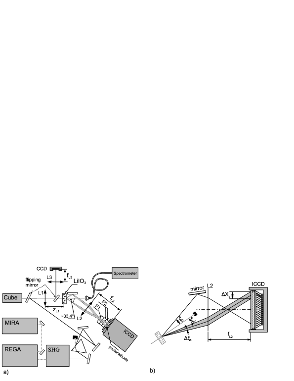
Figure 1: Experimental setup used for the measurement of angular uncertainties: (a) Whole setup using both pumping options and diagnostics of the pump beam (see the text for detailed description); (b) Part of the setup mapping propagation angles behind the nonlinear crystal to the positions on the photocathode.

In our experiment we focused on degenerate photon pairs $\lambda_{s0}=\lambda_{i0}=800$ nm that were emitted on a cone layer with apex angle 33.4 deg behind the crystal. One section of the cone layer was captured directly by the detector, the opposite section was directed to the detector using a high-reflectivity mirror (see Fig. 2a). The detector was composed of an iCCD camera with image intensifier (PI-MAX:512-HQ, Princeton Instruments) preceded by a converging lens L2, one narrow-bandwidth and two high-pass edge filters. The purpose of lens L2 is to map the photon propagation direction angles to positions at the photocathode (see Fig. 2b). Several lenses L2 with focal lengths $f_{L2}$= 12.5, 15, or 25 cm were used in different variants of the experiment. Lens L2 was placed such that the photocathode lied in its focal plane. Filter 11 nm wide was centered at 800 nm. Edge filters (Andover, ANDV7862) blocked wavelengths below 666 nm while their transmittance at 800 nm reached 98%.

Photosensitive area of the detector in the form of a rectangular shape 12.36 mm wide was divided into $512\times 512$ pixels. Resolution of the camera was limited to 38 $\mu$m (FWHM) mainly due to imperfect contrast transfer in the image intensifier. To speed-up the data collection we decreased the resolution even further by grouping $4\times 4$ or $8\times 8$ pixels into one super-pixel in the hardware of the camera. Typically we captured several tens of camera frames per second. Quantum efficiency of the detector was estimated to 7% including all the components between the nonlinear crystal and photocathode.

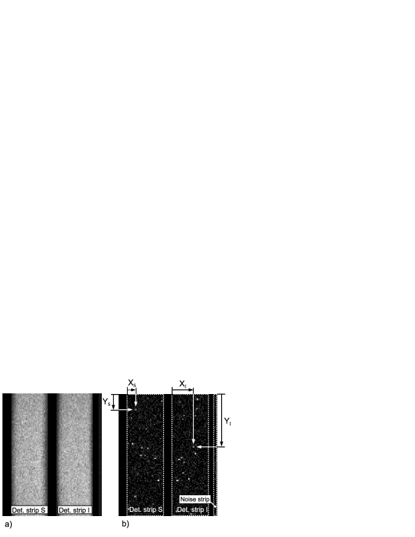
Figure 2: (a) Cumulative registration of photons produced by 20,000 consecutive pump pulses in one camera frame. Signal and idler strips image small sections of the cone layer (note slight curvature of the strips, the curvature is oriented in the same sense for both strips because the idler strip is reflected from a mirror). (b) A typical frame containing photon detection events caused by one pump pulse.

To measure the signal-idler correlation function given in Eq. (2) we defined three regions-of-interest at the iCCD photocathode (see Fig. 2). Two of them capture signal and idler photons and their widths are given by bandwidth filter and lens L2 focal length. The third strip serves for monitoring the noise level. In a pulsed regime a 10 ns long gate of the camera was used synchronously with laser pulses. Considering cw pumping the camera was triggered internally with a gate lasting 2 $\mu$s. Pump-field intensity was set so that the average number of photon detection events per signal/idler strip was much lower than the number of super-pixels in each strip ($\sim 5000$). This made the probability of detecting two photons in a single super-pixel negligible.

Not all detection events were due to signal or idler photons. We made a detailed analysis of the noise and found out that 1.82% of detections came from noise the majority of which (9/10) were red photons coming from fluorescence in the crystal. The rest were scattered pumping photons and only 1.6% of the noise was caused by dark counts.

Evaluation of the detection frames allowed us to compute the experimental correlation function in the horizontal ($X$) and vertical ($Y$) coordinates at the camera (see Fig. 2b) as follows:

$$g\left({X_{S},X_{I}}\right)=\sum\limits_{p=1}^{N}{}\sum\limits_{m=1}^{M_{p}}{}\sum\limits_{l=1}^{L_{p}}{\frac{1}{{M_{p}L_{p}}}}\,\delta\left({X_{S}^{pm}-X_{S}}\right)\delta\left({X_{I}^{pl}-X_{I}}\right),$$ (4)

where $p$ is an index of the frame ($N$ gives the number of frames) and $m$ ($l$) counts signal (idler) detection events [up to $M_{p}$ ($L_{p}$) in the $p$-th frame]. Symbol $X_{s}^{pl}$ [$X_{i}^{pl}$] denotes horizontal position of the $l$-th detection in the signal [idler] strip in the $p$-th frame. Correlations in the vertical direction are determined similarly. In this way, all possible combinations of pairwise detection events are taken into account.

4 Results

A typical result for pulsed pumping based on a measurement sequence lasting three hours is given in Fig. 3.

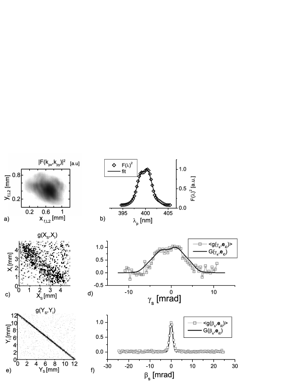
Figure 3: Results of a typical measurement sequence with pulsed pumping containing 327,600 frames, $L_{cr}=5$ mm. (a) Spatial spectrum of the pump beam as measured in lens L3 focal plane. (b) Intensity spectrum of the pump beam; diamonds are experimental values from spectrometer, solid line is a multi-peak Gaussian fit. (c,e) Experimental correlation functions $g(X_{S},X_{I})$ and $g(Y_{S},Y_{I})$ evaluated according to Eq. (4). (d,f) Cross-sections of functions $g(X_{S},X_{I})$ and $g(Y_{S},Y_{I})$ along the signal axis averaged over all registered idler values (open rectangles) and the corresponding theoretical curves $G$ given by Eq. (2) obtained from the numerical model (solid lines). These plots are cast in angular units $\gamma_{s}\approx X_{s}/f_{L2}$, $\beta_{s}\approx Y_{s}/f_{L2}$.

Spatial spectrum of the pump beam as measured in the focal plane of lens L3 is shown in Fig. 3a and the corresponding intensity spectral profile in Fig. 3b. Plots of the correlation functions $g(X_{S},X_{I})$ and $g(Y_{S},Y_{I})$ evaluated from 327,000 registered frames according to Eq. (4) are given in Figs. 3c and 3e. Pairwise correlated character of the fields leads to the diagonal patterns going from upper-left to lower-right corners of the plots. The diagonals have finite widths originating in spreading of signal propagation directions related to one fixed idler direction. We denote half-widths of the diagonals as $\Delta X_{s}/2$ and $\Delta Y_{s}/2$ or, in angular quantities, as $\Delta\gamma_{s}/2\approx\Delta X_{s}/(2f_{L2})$ and $\Delta\beta_{s}/2\approx\Delta Y_{s}/(2f_{L2})$. Since these widths apparently do not change significantly in the $X$ and $Y$ ranges used for plotting Figs. 3c and 3e, we can increase the precision in determining $\Delta\gamma_{s}$ and $\Delta\beta_{s}$ by averaging over the range of measured idler coordinates. The averaged cross-sections along signal coordinates $\gamma_{s}$ and $\beta_{s}$ are indicated by angle brackets $\langle\rangle$ and are plotted in Figs. 3d and 3f (open rectangles). Here, solid lines show the corresponding curves giving $G(\mathbf{k}_{s},\mathbf{k}_{i0})$ that are obtained from the numerical model using parameters of the pump beam as were derived from the measurements reported in Figs. 3a and 3b. Excellent agreement of the model with experimental data is evident even though the pump-field spatial shape and its spectrum are nontrivial.

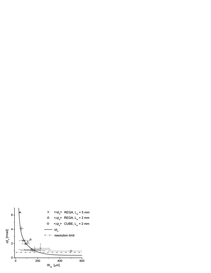
Figure 4: Dependence of vertical angular uncertainty $\langle\Delta\beta_{s}\rangle$ on the bandwidth of vertical pump-beam waist $W_{y0}$ for pulsed (crosses and triangles) and cw (diamonds) pumping. Two different crystal lengths were used: 5 mm (crosses) or 2 mm (triangles and diamonds). Solid line is provided by the numerical model. Dash-dot horizontal line indicates the resolution limit given by camera super-pixel size.

We have performed systematic investigation of the dependencies of angular uncertainty $\langle\Delta\beta_{s}\rangle$ on various parameters of the pump beam and crystal length. The role of vertical dimension of the pump-beam waist $W_{y0}$ in the behavior of the uncertainty $\langle\Delta\beta_{s}\rangle$ is revealed in Fig. 4 where values for both pumping options and two different crystal lengths are plotted on the top of the solid line given by the numerical model. We note that in this case and according to the model values of the uncertainty $\langle\Delta\beta_{s}\rangle$ do not change with pump spectral width and horizontal beam-waist size $W_{x0}$. We can see in Fig. 4 that experimental points follow the theoretical curve except for the area of narrow diagonals where the experimental resolution was limited by the size of super-pixels.

5 Conclusions

Thanks to the ability of the intensified CCD camera to register single-photon detection events and positions of their occurrence, we were able to measure angular uncertainties of the far-field signal-idler correlations in the process of parametric fluorescence in an LiIO₃ nonlinear crystal. In particular, we have measured the dependence of vertical angular uncertainty on the vertical pump-beam waist size using both cw and pulsed pumping and two different crystal lengths. We have reached a very good agreement with the numerical model of parametric fluorescence that simulates the process for any polychromatic elliptical pump beam.

References

- [1] T. G. Giallorenziho, C. L. Tang, Phys. Rev. 166, 225 (1968).
- [2] C. K. Hong, L. Mandel, Phys. Rev. A 31, 2409 (1985).
- [3] L. J. Wang, X. Y. Zou, L. Mandel, Phys. Rev. A 44, 4614 (1991).
- [4] T. P. Grayson, G. A. Barbosa, Phys. Rev. A. 49, 2948 (1994).
- [5] O. Steuernagel, Rabitz H., Opt. Commun. 154, 285 (1998).
- [6] T. E. Keller, M. H. Rubin, Phys. Rev. A 56, 1534 (1997).
- [7] J. Peřina, Jr., A. V. Sergienko, B. M. Jost, B. E. A. Saleh, M. C. Teich, Phys. Rev. A 59, 2359 (1999).
- [8] A. Joobeur, B. E. A. Saleh, M. C. Teich, Phys. Rev. A 50, 3349 (1994).
- [9] A. Joobeur, B. E. A. Saleh, T. S. Larchuk, M. C. Teich, Phys. Rev. A 53, 4360 (1996).
- [10] Y. Shih, Rep. Prog. Phys. 66, 1009 (2003).
- [11] J. Peřina, M. Centini, C. Sibilia, M. Bertolotti, M. Scalora, Phys. Rev A 73, 033823 (2006).
- [12] J. Peřina Jr., Phys. Rev A 77, 013803 (2008).