The spectral distance in the Moyal plane

Abstract

We study the noncommutative geometry of the Moyal plane from a metric point of view. Starting from a non compact spectral triple based on the Moyal deformation $\mathcal{A}$ of the algebra of Schwartz functions on $\mathbb{R}^{2}$, we explicitly compute Connes’ spectral distance between the pure states of $\mathcal{A}$ corresponding to eigenfunctions of the quantum harmonic oscillator. For other pure states, we provide a lower bound to the spectral distance, and show that the latest is not always finite. As a consequence, we show that the spectral triple [19] is not a spectral metric space in the sense of [5]. This motivates the study of truncations of the spectral triple, based on $M_{n}(\mathbb{C})$ with arbitrary $n\in\mathbb{N}$, which turn out to be compact quantum metric spaces in the sense of Rieffel. Finally the distance is explicitly computed for $n=2$.

^aLaboratoire de Physique Théorique, Bât. 210
Université Paris-Sud 11, 91405 Orsay Cedex, France
e-mail: eric.cagnache@th.u-psud.fr, jean-christophe.wallet@th.u-psud.fr
^bDépartement de Mathématiques, Université Catholique de Louvain
Chemin du cyclotron 2, 1348 Louvain-La-Neuve, Belgium
e-mail: francesco.dandrea@uclouvain.be
^cInstitut für Theoretische Physik, Georg-August Universität
Friedrich-Hund-Platz 1, 37077 Göttingen, Germany
^dCourant Center “Higher Order Structures in Mathematics”, Universität Göttingen
Busenstr. 3-5, 37073 Göttingen, Germany
e-mail: martinetti@theorie.physik.uni-goettingen.de

1 Introduction

Mainly motivated by quantum mechanics, where physical quantities are no longer functions on a manifold as in classical mechanics but elements of a noncommutative operator algebra, Noncommutative Geometry [9] aims at describing “spaces” in terms of algebras $\mathcal{A}$ rather than as sets of points. Many examples of noncommutative spaces are known (e.g. almost commutative manifolds [25], fuzzy spaces [32], deformations for actions of $\mathbb{R}^{n}$ [38], Drinfel’d-Jimbo [17, 27], Connes-Landi [13] and Connes-Dubois-Violette [12] deformations), but little work has been done regarding their metric aspect. Let us recall that in Connes theory a natural distance [14] on the state space ${\cal S(\mathcal{A})}$ of $\mathcal{A}$ is obtained via the construction of a spectral triple (cf. Sec. 2.2), the latest providing a noncommutative generalization of many tools of differential geometry [11]. In this paper we focus on the associated distance, whose definition is recalled in Def. 3.1, from now on called the spectral distance.

On a (finite dimensional, complete) Riemannian spin manifold $M$, the spectral distance $d$ between pure states of the commutative algebra $C_{0}^{\infty}(M)$ of smooth functions vanishing at infinity coincides with the geodesic distance between the corresponding points, while $d$ between non-pure states coincides with the Wasserstein distance of order $1$ between the corresponding probability distributions [16]. In the noncommutative case, the meaning of the spectral distance is still obscure, essentially due to a lack of examples: $d$ has been explicitly computed only for finite dimensional noncommutative algebras (e.g. [26, 6]) and almost commutative geometries [34, 35] where it exhibits some interesting links with the Carnot-Carathéodory distance in sub-Riemannian geometry [33]. To shed more light on the spectral distance in a noncommutative framework, a natural idea is to investigate the motion of a quantum particle along a line which, from a mathematical point of view, amounts to studying the well known Moyal plane. An associated spectral triple has been proposed in [19], built around the algebra $\mathcal{A}$ of Schwartz functions on $\mathbb{R}^{2}$ equipped with the Moyal product $\star$. Although this spectral triple is an isospectral deformation of the canonical spectral triple of the Euclidean plane, the spectral distance $d$ on the Moyal plane does not appear to be a deformation of the Euclidean distance on $\mathbb{R}^{2}$. It has rather a quantum mechanics interpretation. Indeed the pure states ${\cal P(\mathcal{A})}$ of $\mathcal{A}$ correspond to Wigner transition eigenfunctions of the quantum harmonic oscillator, and we show in this paper (Proposition 3.6) that the eigenstates of the quantum harmonic oscillator form a $1$-dimensional lattice of the Moyal plane, with distance between two subsequent energy levels $E_{m-1},E_{m}$ proportional to $m^{-\frac{1}{2}}$. We also point out some states at infinite distance from one another, meaning that the topology induced by $d$ on ${\cal S(\mathcal{A})}$ is not the weak^∗ topology. Therefore the spectral triple for the Moyal plane introduced in [19] is not a spectral metric space [31, 5]. This leads us to study truncations of the Moyal spectral triple, which turn out to be compact quantum metric spaces in the sense of Rieffel [39, 40].

The paper is organized as follows. In section 2 we recall some basics on the Moyal product, the associated spectral triple, the pure states of the Moyal algebra and we establish several technical results. In section 3, we explicitly compute the spectral distance between the eigenstates of the quantum harmonic oscillator. We also derive some bounds for the distance between any pure states and show that the induced topology is not the weak^∗ topology. In section 4 we introduce a spectral triple on $M_{n}(\mathbb{C})$ obtained by truncating the Moyal spectral triple. We explicitly compute the associated spectral distance for $n=2$, and for $n\geq 2$ we prove that the truncation gives a compact quantum metric space (Proposition 4.2). This is an interesting result since the “natural” spectral triple on $M_{n}(\mathbb{C})$ studied in [26] did not induce a quantum metric space. In Section 5 we draw conclusions and illustrate open problems.

2 Moyal non compact spin geometries

2.1 Moyal product, matrix basis and relevant algebras of tempered
distribution on $\mathbb{R}^{2}$

The main properties of the Moyal machinery can be found e.g. in [21, 22] to which we refer for more details. Various related algebras have appeared in the literature, some of which will be recalled below. An extension of Connes real spectral triple to the non-compact case, to which we will refer heavily throughout this paper, has been carried out in [19]; the corresponding action functionals and spectral actions have also been considered in [18]. Constructions of various derivation based differential calculi on Moyal algebras have been carried out in [8, 44, 20] together with applications to the construction of Yang-Mills-Higgs models on non-commutative Moyal spaces. In this work, we will only consider the 2-dimensional case.

Let ${\cal{S}}={\cal{S}}({\mathbb{R}}^{2})$ be the space of complex Schwartz functions on ${\mathbb{R}}^{2}$ and ${\cal{S}}^{\prime}={\cal{S}}^{\prime}({\mathbb{R}}^{2})$ its topological dual. Let $\theta>0$ be a fixed positive real parameter.

Proposition 2.1.

[37, 23] The associative Moyal $\star-$product is defined for all $a,b$ in ${\cal{S}}$ by $\star:{\cal{S}}\times{\cal{S}}\to{\cal{S}}$

$$(a\star b)(x)=\frac{1}{(\pi\theta)^{2}}\int d^{2}y\,d^{2}z\ a(x+y)b(x+z)e^{-i\,2y\,\Theta^{-1}z},$$ (2.1)

$$\text{ where }\;y\,\Theta^{-1}z\equiv y^{\mu}\Theta^{-1}_{\mu\nu}z^{\nu},\ \Theta_{\mu\nu}=\theta\begin{pmatrix}0&1\\ -1&0\end{pmatrix}.$$

The complex conjugation is an involution for the $\star$-product; the integral is a faithful trace,

$$\int d^{2}x\ (a\star b)(x)=\int d^{2}x\ (b\star a)(x)=\int d^{2}x\ a(x)b(x);$$

the Leibniz rule is satisfied: $\partial_{\mu}(a\star b)=\partial_{\mu}a\star b+a\star\partial_{\mu}b$, $\forall a,b\in{\cal{S}}$.

In all the paper, we denote

$${\cal{A}}:=({\cal{S}},\star)$$ (2.2)

the non-unital involutive algebra of Schwartz functions equipped with the Moyal product.

Our analysis will use the matrix basis whose relevant properties are summarized below.

Proposition 2.2.

[21] The matrix basis $\{f_{mn}\}_{m,n\in\mathbb{N}}\subset{\cal{S}}\subset L^{2}({\mathbb{R}}^{2})$ is the family of Wigner transition eigenfunctions of the 1-dimensional harmonic oscillator,

$$f_{mn}={\frac{1}{(\theta^{m+n}m!n!)^{1/2}}}\;{\bar{z}}^{\star m}\star f_{00}\star z^{\star n}$$

where $f_{00}=2e^{-2H/\theta}$, $H={\frac{1}{2}}(x_{1}^{2}+x_{2}^{2}),$ $X^{\star n}=\underset{n\text{ times}}{\underbrace{X\star X\star...\star X}}$ and

$${\bar{z}}={\tfrac{1}{{\sqrt{2}}}}(x_{1}-ix_{2}),\qquad z={\tfrac{1}{{\sqrt{2}}}}(x_{1}+ix_{2}).$$ (2.3)

i) Writing $\langle.,.\rangle$ the inner product on $L^{2}({\mathbb{R}}^{2})$, one has the relations

$$f_{mn}\star f_{pq}=\delta_{np}f_{mq},\qquad f_{mn}^{*}=f_{nm},\qquad\langle f_{mn},f_{kl}\rangle=(2\pi\theta)\delta_{mk}\delta_{nl}.$$

ii) $\mathcal{A}$ is a Fréchet pre-$C^{*}$-algebra, with seminorms $\rho_{\alpha\beta}(a)=\sup_{x\in{\mathbb{R}}^{2}}\lvert x^{\beta}D^{\alpha}a\rvert,$ isomorphic to the Fréchet algebra of rapid decay matrices $(a_{mn})_{m,n\in{\mathbb{N}}}$ with seminorms

$$\rho_{k}^{2}(a):=\sum_{m,n\in{\mathbb{N}}}\theta^{2k}(m+\tfrac{1}{2})^{k}(n+\tfrac{1}{2})^{k}|a_{mn}|^{2}.$$ (2.4)

The isomorphism is given by $(a_{mn})\rightarrow\sum_{m,n}a_{mn}f_{mn}\in{\cal{S}}$, with inverse

$$a\in{\cal{S}}\rightarrow a_{mn}={\frac{1}{2\pi\theta}}\langle f_{mn},a\rangle={\frac{1}{2\pi\theta}}\int d^{2}x\,a(x)f_{mn}^{*}(x)={\frac{1}{2\pi\theta}}\int d^{2}x\,a(x)f_{nm}(x).$$

The matrix basis diagonalizes the Hamiltonian of the harmonic oscillator,

$$H\star f_{mn}=\theta(2m+1)f_{mn},\;\qquad f_{mn}\star H=\theta(2n+1)f_{mn},$$

and is also called the twisted Hermite basis (an explicit decomposition on the Hermite functions $h_{m}$ is provided by the Wigner operator $W(f_{mn})=h_{m}\otimes h_{n}$, see [21] and references therein). In particular the $f_{mm}$, $m\in\mathbb{N}$, are the eigenstates of the $m^{\text{th}}$ energy level of the harmonic oscillator, and in Proposition 3.6 below we compute the spectral distance between any two of them. In a different context, the authors of [3] and [2] have used $H$ as (the square of) a distance-operator, yielding a notion of quantized-distance in the Moyal plane which is distinct from the spectral distance. The link between these two approaches will be the object of a future work [36]. For subsequent computations, let us write the derivatives of the the $f_{mn}$, that are obtained by easy calculation.

Proposition 2.3.

Define $\partial={\frac{1}{{\sqrt{2}}}}(\partial_{1}-i\partial_{2})$, ${\bar{\partial}}={\frac{1}{{\sqrt{2}}}}(\partial_{1}+i\partial_{2})$. For any $m,n\in{\mathbb{N}}$

$$\partial f_{mn}={\sqrt{{\frac{n}{\theta}}}}f_{m,n-1}-{\sqrt{{\frac{m+1}{\theta}}}}f_{m+1,n};\ {\bar{\partial}}f_{mn}={\sqrt{{\frac{m}{\theta}}}}f_{m-1,n}-{\sqrt{{\frac{n+1}{\theta}}}}f_{m,n+1}.$$

The $\star$ product (2.1) is extended to spaces larger than ${\cal{S}}$, obtained by completing the Schwartz algebra with respect to the norm

$$||a||_{s,t}^{2}=\sum\nolimits_{m,n}\theta^{s+t}(m+\tfrac{1}{2})^{s}(n+\tfrac{1}{2})^{t}|a_{mn}|^{2}$$

with $s,t\in{\mathbb{R}}$. Calling ${\cal{G}}_{s,t}$ the completion, one has that for any $a\!=\!\sum_{m,n}a_{mn}f_{mn}\in{\cal{G}}_{s,t}$, $b\!=\sum_{m,n}b_{mn}f_{mn}\in{\cal{G}}_{q,r}$ with $t+q\geq 0$, the sequence $c_{mn}=\sum_{p}a_{mp}b_{pn}$ converges in ${\cal{G}}_{s,r}$, thus defining a map $\star:{\cal{G}}_{s,t}\times{\cal{G}}_{q,r}\rightarrow{\cal{G}}_{s,r}.$ In particular ${\cal{G}}_{0,0}=L_{2}(\mathbb{R}^{2})$ and one has the dense inclusions ${\cal{S}}\subset{\cal{G}}_{s,t}\subset{\cal{S}}^{\prime}$ for any $s,t\in\mathbb{R}$. Using continuity and duality of $\star$ (for more details, see e.g. [21, 22]) one can define the star product on various subspaces of ${\mathcal{S}^{\prime}}$. The following algebras in particular are relevant for the study of Moyal spaces.

Proposition 2.4.

[19] Let ${\cal{D}}_{L^{2}}$ denote the space of square integrable smooth functions on ${\mathbb{R}}^{2}$ having all their derivatives in $L^{2}({\mathbb{R}}^{2})$, ${\cal{B}}$ the space of smooth functions on $\mathbb{R}^{2}$ that are bounded together with all their derivatives and

$${\mathbf{A}}_{\theta}=\{a\in{\cal{S}}^{\prime}\;/\;a\star b\in L^{2}({\mathbb{R}}^{2}),\ \forall b\in L^{2}({\mathbb{R}}^{2})\}\;.$$

i) ${\mathbf{A}}_{\theta}$ is a unital C*-algebra with operator norm

$$||a||_{\theta}=\left\lVert L(a)\right\rVert_{op}=\sup_{0\neq b\in L^{2}({\mathbb{R}}^{2})}\left\{{\frac{||a\star b||_{2}}{||b||_{2}}}\right\}\quad\forall a\in{\mathbf{A}}_{\theta},$$ (2.5)

where $L(.)$ is the left multiplication operator and $||.||_{2}$ denotes the $L^{2}({\mathbb{R}}^{2})$ norm. Moreover ${\mathbf{A}}_{\theta}$ is isomorphic to the algebra of bounded operators on $L^{2}({\mathbb{R}})$.

ii) $({\cal{D}}_{L^{2}},\star)$ is a Fréchet sub-algebra of $({\mathbf{A}}_{\theta},\star)$, with Fréchet topology of $L^{2}({\mathbb{R}}^{2})$-convergence for all derivatives; $({\cal{B}},\star)$ is a Fréchet sub-algebra of $({\mathbf{A}}_{\theta},\star)$, with topology given by the family of semi-norms $\{p_{m}\}_{m\in{\mathbb{N}}},\ p_{m}(a):=\text{max}_{\lvert\alpha\rvert<m}||\partial^{\alpha}(a)||_{\infty}$.

iii) $({\cal{D}}_{L^{2}},\star)$ and $({\cal{B}},\star)$ are respectively non unital and unital pre C*-algebras with respect to $\left\lVert.\right\rVert_{\theta}$. Denoting by an over-bar their $C^{*}$-completions, one has the inclusions

$$\mathcal{A}\subset\bar{\cal D}_{L^{2}}\subset\bar{\cal B}\subset{\mathbf{A}}_{\theta}.$$ (2.6)

The above algebras are related but not identical to the maximal unitization ${\cal{M}}=({\cal{M}}_{L}\cap{\cal{M}}_{R},\star)$ of $\mathcal{A}$ underlying most of the studies on noncommutative field theories and noncommutative gauge theories on Moyal spaces (see e.g. [24, 42, 8, 44, 20] and references therein), where

$${\cal{M}}_{L}:=\{a\in{\cal{S}}^{\prime}\ /\ a\star b\in{\cal{S}},\ \forall b\in{\cal{S}}\},\qquad{\cal{M}}_{R}:=\{a\in{\cal{S}}^{\prime}\ /\ b\star a\in{\cal{S}},\ \forall b\in{\cal{S}}\}.$$

${\cal{M}}$ is unsuitable here as it cannot be represented by bounded operators on the Hilbert space $L^{2}(\mathbb{R}^{2})\otimes\mathbb{C}^{2}$ used in the non-compact spectral triple that we now recall.

2.2 Spectral triple for Moyal plane

A unital spectral triple [9] is the datum of a unital involutive algebra $A$ together with a representation $\pi$ on an Hilbert space $\mathcal{H}$ and a selfadjoint not necessarily bounded operator $D$ (called Dirac operator) on $\mathcal{H}$, such that $[D,\pi(a)]$ is bounded for any $a\in A$ and the resolvent of $D$ is compact. In the non compact case, i.e. for non-unital $A$, one asks instead [10] that the operators $\pi(a)(D-\lambda)^{-1}$ are compact for any $\lambda\notin\text{Sp }D$. A natural candidate-spectral-triple for the Moyal plane is the isospectral deformation [13] of the canonical spectral triple of the Euclidean plane ${\mathbb{R}}^{2}$ built around the algebra of Schwartz functions; namely

$$({\cal{A}},{\cal{H}},D)$$ (2.7)

with $\mathcal{A}$ defined in (2.2),

$${\cal{H}}=L^{2}({\mathbb{R}}^{2})\otimes{\mathbb{C}}^{2}\equiv{\cal{H}}_{0}\otimes{\mathbb{C}}^{2}$$

the Hilbert space of square integrable sections of the trivial spinor bundle ${\mathbb{S}}={\mathbb{R}}^{2}\times{\mathbb{C}}^{2}$ with inner product

$$\langle\psi,\phi\rangle=\int(\psi_{1}^{*}\phi_{1}+\psi_{2}^{*}\phi_{2})d^{2}x\quad\forall\;\psi=\binom{\psi_{1}}{\psi_{2}},\;\phi=\binom{\phi_{1}}{\phi_{2}}\;\in{\cal{H}},$$

and, using Einstein convention of summing over repeated indices,

$$D=-i\sigma^{\mu}{\partial}_{\mu}=-i{\sqrt{2}}\begin{pmatrix}0&{{\bar{\partial}}}\\ {\partial}&0\end{pmatrix}$$ (2.8)

where

$$\sigma^{1}=\begin{pmatrix}0&1\\ 1&0\end{pmatrix},\qquad\sigma^{2}=\begin{pmatrix}0&i\\ -i&0\end{pmatrix}$$

span an irreducible representation of the Clifford algebra $C\ell_{2}(\mathbb{C})=M_{2}(\mathbb{C})$. ${\cal{A}}$ acts faithfully on ${\cal H}$ via the representation $\pi(a)=L(a)\otimes\mathbb{I}_{2}$, namely

$$\pi(a)\psi=(a\star\psi_{1},a\star\psi_{2})\quad\forall a\in\mathcal{A},\psi\in\mathcal{H}.$$ (2.9)

(2.7) does satisfy the property of a non-compact spectral triple: $\pi(a)$ is bounded by (2.9) and (2.6) together with ${\mathbf{A}}_{\theta}\simeq{\cal{B}}(L^{2}(\mathbb{R}))$. The boundedness of $[D,\pi(a)]$ comes from $[D,\pi(a)]=-iL(\partial_{\mu}a)\otimes\sigma^{\mu}$, see (3.6), combined with $L(\partial_{\mu}a)\in{\cal{B}}(L^{2}(\mathbb{R}))$. $D$ is the usual Dirac operator on $\mathbb{R}^{2}$ so it is essentially selfadjoint. Note that $D$ being formally selfadjoint on its domain ${\cal{D}}_{L^{2}}\otimes{\mathbb{C}}^{2}$ can be easily seen noticing that the adjoint of ${\partial}$ is ${\partial}^{\dagger}=-{{\bar{\partial}}}$. The resolvent condition is more involved and we refer to [19] for the details.

In order to establish the equivalence between (unital) commutative spectral triples and (compact, oriented, without boundary) smooth manifolds, one further asks five extra-conditions on $(\mathcal{A},{\cal H},D)$ [11] (dimension, order one, regularity, orientability, finiteness), that can be completed by two other conditions (reality, Poincaré duality) in order to recover spin and Riemannian structures from purely algebraic data. This yields the definition of real spectral triples [10]. Among these conditions, several easily translate to the non-compact case (dimension, regularity, reality, first order condition), one still asks a formulation in the non-compact case (Poincaré duality). For the remaining two (finiteness, orientability), an adaptation to the non-unital case has been proposed in [19], based on a preferred unitization ${\cal{A}}_{1}:=({\cal{B}},\star)$ of ${\cal{A}}$. However, as can be checked in Definition 3.1 below, none of these conditions enters the definition of the spectral distance. So, regarding the metric aspect of the Moyal plane, it is more natural to work with the spectral triple (2.7) as we do in the following than with the unitization ${\cal A}_{1}$. We come back to this point in section 4 and in the conclusion.

3 Spectral distance on the Moyal plane

3.1 Distance formula and pure states

Let us begin with a technical precision. A state on a complex $C^{*}$-algebra $A$ is a positive linear map $A\rightarrow{\mathbb{C}}$ of norm $1$, and strictly speaking this notion is reserved for $C^{*}$-algebras. However given a pre $C^{*}$-algebra $A$, a state on its $C^{*}$-completion $\bar{A}$ defines by restriction a unique positive linear map of norm $1$ from $A$ to ${\mathbb{C}}$, and conversely by continuity any state of $\bar{A}$ is uniquely determined by its restriction to $A$. So it is also legitimate to talk about states for pre $C^{*}$-algebras.

The metric aspect of the noncommutative geometry $({\mathcal{A}},{\mathcal{H}},D)$ introduced in (2.7) is fully encoded within the spectral distance defined as follows.

Definition 3.1.

The spectral distance between two states $\omega_{1}$ and $\omega_{2}$ of $\mathcal{A}$ is

$$d(\varphi_{1},\varphi_{2})=\sup_{a\in\mathcal{A}}\big{\{}|\varphi_{1}(a)-\varphi_{2}(a)|;\ ||[D,\pi(a)]||_{\text{op}}\leq 1\big{\}}$$ (3.1)

where $||.||_{\text{op}}$ is the operator norm for the representation of ${\cal{A}}$ in ${\cal{B}}({\cal{H}})$.

One easily checks that (3.1) has all the properties of a distance, except that it may take the value $+\infty$. Recall that in the commutative case, i.e. $\mathcal{A}=C^{\infty}_{0}(M)$ for $M$ a complete Riemannian spin manifold, $\mathcal{H}$ the space of spinors square-integrable with respect to the volume form associated to the Riemannian metric, and $D$ the Dirac operator of the Levi-Civita connection, then pure states are evaluations at $x\in M$:

$$\delta_{x}(f)=f(x)\quad\forall f\in C^{\infty}_{0}(M),$$ (3.2)

and $d(\delta_{x},\delta_{y})$ coincides with the geodesic distance on $M$. Therefore it is appealing, in the noncommutative case, to consider the spectral distance between pure states as a good equivalent of the geodesic distance between points.

However, on the deformed algebra $\mathcal{A}$ the evaluation (3.2) is no longer a state, for $(f^{*}\star f)(x)$ has no reason to be positive. Having in mind Moyal spaces as a quantized version of Euclidean spaces, one could be tempted to look at the pure states of $\mathcal{A}$ as a deformation of the pure states of $C^{\infty}_{0}(\mathbb{R}^{2})$. A nice approach on how to obtain states for a Rieffel deformation of a $C^{*}$-algebra by deformation of states of the undeformed algebra has been developed in [30], but the “purity” of the state is not addressed there. In fact, rather than using the $x$-representation (2.1), pure states of $\mathcal{A}$ are more easily determined in the twisted Hermite basis $\left\{f_{mn}\right\}_{m,n\in\mathbb{N}}$.

Let $e_{n}$ be the canonical orthonormal basis of $\ell^{2}(\mathbb{N})$ and $\eta$ the natural representation of rapid decay matrices, given by row by column multiplication. By Prop. 2.2 the isometry $L^{2}(\mathbb{R}^{2})\to\ell^{2}(\mathbb{N})\otimes\ell^{2}(\mathbb{N})$ given by

$$U:f_{mn}\mapsto\sqrt{2\pi\theta}\,e_{m}\otimes e_{n}$$

is an intertwiner between the left regular representation $L$ and the representation $\eta\otimes 1$. One can see that $\eta$ is faithful and irreducible, while $L$ is only faithful (it is the direct sum of infinitely many copies of $\eta$, in the same way as the left regular representation of $M_{n}(\mathbb{C})$ with Hilbert-Schmidt inner product is unitary equivalent to the direct sum of $n$ copies of the irreducible representation). Therefore

$$\mathcal{A}\simeq L(\mathcal{A})\simeq\eta(\mathcal{A})\;.$$

Since the norm of any operator $a$ on $\ell^{2}(\mathbb{N})$ coincides with the norm of $a\otimes 1$ on $\ell^{2}(\mathbb{N})\otimes\ell^{2}(\mathbb{N})$, the closure of $L(\mathcal{A})$ in $\mathcal{B}(L^{2}(\mathbb{R}^{2}))$ is isometrically $*$-isomorphic to the closure of $\eta(\mathcal{A})$ in $\mathcal{B}(\ell^{2}(\mathbb{N}))$: we call $\bar{\mathcal{A}}$ this $C^{*}$-algebra.

Notice that

$$\bar{\mathcal{A}}\supset\eta(\mathcal{A})\supset M_{\infty}(\mathbb{C}):=\bigcup\nolimits_{k\geq 1}M_{k}(\mathbb{C})$$

where $M_{k}(\mathbb{C})$ are identified with $a=((a_{mn}))\in\mathcal{A}$ such that $a_{mn}=0$ if $m\geq k$ or $n\geq k$. By [4, II.8.2.2] the closure of $M_{\infty}(\mathbb{C})$ is the $C^{*}$-algebra $\mathbb{K}$ of compact operators on $\ell^{2}(\mathbb{N})$, proving that $\bar{\mathcal{A}}=\overline{\eta(\mathcal{A})}\supset\mathbb{K}$. On the other hand, $\eta$ maps any rapid decay matrix $a$ into a Hilbert-Schmidt operator, since the norm $\rho_{0}(a)$ in (2.4) is exactly the Hilbert-Schmidt norm of $\eta(a)$. Hence $\eta(a)$ is a compact operator for any $a\in\mathcal{A}$ and $\overline{\eta(\mathcal{A})}\subset\mathbb{K}$, proving that $\bar{\mathcal{A}}\simeq\mathbb{K}$.

It is well known [28, Cor. 10.4.4] that all pure states of $\mathbb{K}$ are vector states of the (unique) irreducible representation on $\ell^{2}(\mathbb{N})$. Hence,

Proposition 3.2.

Any unit vector $\psi=\sqrt{2\pi\theta}\sum_{m}\psi_{m}e_{m}\in\ell^{2}(\mathbb{N})$, i.e. with normalization $\sum_{m}|\psi_{m}|^{2}=\frac{1}{2\pi\theta}$, defines a pure state $\omega_{\psi}$ of $\mathcal{A}$,

$$\omega_{\psi}(a):=2\pi\theta\sum_{m,n\in{\mathbb{N}}}\psi^{*}_{m}\psi_{n}a_{mn}.$$ (3.3)

Moreover any pure state of $\mathcal{A}$ comes from such a unit vector.

Notice that $\psi$ can be obtained from

$$v_{n}:=U^{*}(\psi\otimes e_{n})=\sum\nolimits_{m\geq 0}\psi_{m}f_{mn}$$ (3.4)

for any $n\in\mathbb{N}$, and we have $\omega_{\psi}(a)\equiv\left<v_{n},L(a)v_{n}\right>$.

3.2 Unit ball

In order to compute the distance (3.1) on the Moyal plane, one needs to conveniently characterize the unit ball

$${\mathcal{B}}_{D}:=\left\{a\in\mathcal{A},\,||[D,\pi(a)]||_{\text{op}}\leq 1\right\}.$$ (3.5)

The first step is to determine the relation between the coefficients of $a$ in the matrix basis and those of $[D,\pi(a)]$. Noticing that $[\partial_{\mu},L(a)]=L(\partial_{\mu}a)$ by Leibniz rule one obtains

$$[D,\pi(a)]=-i\sqrt{2}\left(\begin{array}[]{cc}0&L(\bar{\partial}a)\\ L(\partial a)&0\end{array}\right).$$ (3.6)

Thus

$$\left\lVert[D,\pi(a)]\right\rVert_{\text{op}}^{2} =\left\lVert[D,\pi(a)]^{*}[D,\pi(a)]\right\rVert_{\text{op}}=2\left\lVert\begin{pmatrix}L(\partial a)^{*}L(\partial a)&0\\ 0&L(\bar{\partial}a)^{*}L(\bar{\partial}a)\end{pmatrix}\right\rVert_{\text{op}}$$

$$=2\max\left(\left\lVert L(\partial a)^{*}L(\partial a)\right\rVert_{\text{op}},\left\lVert L(\bar{\partial}a)L(\bar{\partial}a)^{*}\right\rVert_{\text{op}}\right)$$

$$=2\max\left(\left\lVert\partial a\right\rVert^{2}_{\theta},\left\lVert\bar{\partial}a\right\rVert^{2}_{\theta}\right)$$ (3.7)

and the point is now to find the relation between the coefficients of $a$ and those of ${\partial}a,{{\bar{\partial}}}a$.

Proposition 3.3.

For any $a\in\mathcal{A}$, $a=\sum_{m,n}a_{mn}f_{mn}$, we denote

$${\partial}a:=\sum_{m,n}\alpha_{mn}f_{mn},\quad{{\bar{\partial}}}a:=\sum_{m,n}{{\beta}}_{mn}f_{mn}.$$

i) The coefficients of ${\partial}a$, ${{\bar{\partial}}}a$ as functions of the coefficients of $a$ are given by

$$\alpha_{m+1,n}={\sqrt{{\frac{n+1}{\theta}}}}a_{m+1,n+1}-{\sqrt{{\frac{m+1}{\theta}}}}a_{m,n},\ \alpha_{0,n}={\sqrt{{\frac{n+1}{\theta}}}}a_{0,n+1},$$ (3.8)

$${{\beta}}_{m,n+1}={\sqrt{{\frac{m+1}{\theta}}}}a_{m+1,n+1}-{\sqrt{{\frac{n+1}{\theta}}}}a_{m,n},\ {{\beta}}_{m,0}={\sqrt{{\frac{m+1}{\theta}}}}a_{m+1,0},$$ (3.9)

for all $m,n\in{\mathbb{N}}$.

ii) One has the inversion formula

$$a_{p,q}=\delta_{p,q}a_{0,0}+\sqrt{\theta}\,\sum_{k=0}^{\min(p,q)}\frac{\alpha_{p-k,q-k-1}+\beta_{p-k-1,q-k}}{\sqrt{p-k}+\sqrt{q-k}},\forall p,q\in{\mathbb{N}},p+q>0$$

where by convention terms with negative indices do not appear in the sum.

Proof.

i) is proved by standard calculation using Proposition 2.3. To prove ii) one combines (3.8) and (3.9) to obtain

$$a_{p+1,q+1}=a_{p,q}+\sqrt{\theta}\,\frac{\alpha_{p+1,q}+\beta_{p,q+1}}{\sqrt{p+1}+\sqrt{q+1}}.$$

This yields by induction

$$a_{p,q}=\begin{cases}a_{0,q-p}+\sqrt{\theta}\,\sum_{k=0}^{p-1}\frac{\alpha_{p-k,q-k-1}+\beta_{p-k-1,q-k}}{\sqrt{p-k}+\sqrt{q-k}}&\text{if}\;0\leq p<q\;,\\ a_{0,0}+\sqrt{\theta}\,\sum_{k=0}^{p-1}\frac{\alpha_{p-k,p-k-1}+\beta_{p-k-1,p-k}}{2\sqrt{p-k}}&\text{if}\;0\leq p=q\;,\\ a_{p-q,0}+\sqrt{\theta}\,\sum_{k=0}^{q-1}\frac{\alpha_{p-k,q-k-1}+\beta_{p-k-1,q-k}}{\sqrt{p-k}+\sqrt{q-k}}&\text{if}\;0\leq q<p\;,\end{cases}$$

and ii) follows from a further use of the second relations for $\alpha_{0,n}$ and $\beta_{0,n}$. ∎

The second step in order to characterize ${\cal B}_{D}$ would be to compute $\left\lVert[D,a]\right\rVert$ as an explicit function $f(\alpha_{mn})$, then use Proposition 3.3 to transfer the constraints $f(\alpha_{mn})\leq 1$ to the coefficients $a_{mn}$. However we are dealing with infinite dimensional matrices and one may well not have such a function $f$. Here we simply exhibit some necessary constraints on the $a_{mn}$’s so that $a\in{\cal B}_{D}$. Quite remarkably these constraints are sufficient to explicitly compute, in the next section, the distance for interesting classes of pure states.

Lemma 3.4.

Let $a\in{\mathcal{B}}_{D}$. Then

i) For any unit vector $\varphi=\sum_{m,n}\varphi_{mn}f_{mn}\in{\cal{H}}_{0}$ one has

$$\sum_{p}|\alpha_{mp}||\varphi_{pn}|\leq{\frac{1}{2{\sqrt{\pi\theta}}}}\;\;and\;\;\sum_{p}|\beta_{mp}||\varphi_{pn}|\leq{\frac{1}{2{\sqrt{\pi\theta}}}},\quad\forall m,n\in{\mathbb{N}};\$$ (3.10)

ii) $|\alpha_{mn}|\leq{\frac{1}{{\sqrt{2}}}}$  and   $|\beta_{mn}|\leq{\frac{1}{{\sqrt{2}}}}$, $\forall m,n\in{\mathbb{N}}.$

Proof.

Let $\varphi$ be a unit vector in $\mathcal{H}_{0}$, that is to say $||\varphi||^{2}_{2}=2\pi\theta\sum_{mn}\lvert\varphi_{mn}\rvert^{2}=1.$ Using the matrix basis, a standard calculation yields

$$||{\partial}a\star\varphi||_{2}^{2}=2\pi\theta\sum_{m,n}\Big{|}\sum_{p}\alpha_{mp}\varphi_{pn}\Big{|}^{2}.$$

By (3.7) $a\in{\mathcal{B}}_{D}\!$ implies $||{\partial}a||_{\theta}\!\leq\!\!{\frac{1}{{\sqrt{2}}}}$ hence, owing to the definition of $||{\partial}a||_{\theta}$,

$$\sum_{m,n}\Big{|}\sum_{p}\alpha_{mp}\varphi_{pn}\Big{|}^{2}\leq{\frac{1}{4\pi\theta}}.$$

This implies

$$\Big{|}\sum_{p}\alpha_{mp}\varphi_{pn}\Big{|}\leq{\frac{1}{2{\sqrt{\pi\theta}}}}\quad\forall m,n\in{\mathbb{N}}$$ (3.11)

together with a similar relation stemming from $||{{\bar{\partial}}}a||_{\theta}$ with the $\alpha_{mn}$’s replaced by $\beta_{mn}$. Now (3.11) holds true for any unit $\varphi\in{\cal{H}}_{0}$ and in particular, given a value $m\in{\mathbb{N}}$, for ${\tilde{\varphi}}^{m}$ defined by $\tilde{\varphi}_{pn}^{m}:=e^{-i\text{Arg}(\alpha_{mp})}\lvert\varphi_{pn}\rvert$. This implies

$$\sum_{p}|\alpha_{mp}||\varphi_{pn}|\leq{\frac{1}{2{\sqrt{\pi\theta}}}},\quad\forall n\in{\mathbb{N}}$$ (3.12)

and the first part of (3.10) by repeating the procedure for other values of $m$. The second part is obtained by similar considerations apply to the $\beta_{mn}$’s. ii) is obtained by considering in (3.12) the unit vector $\varphi=\frac{1}{\sqrt{2\pi\theta}}f_{mn}$. ∎

Notice that by the triangle inequality (3.12) implies (and thus is equivalent to) (3.11).

Remark 3.5.

When the algebra ${\mathcal{A}}$ is unital the supremum in the distance formula can be equivalently searched on the positive unit sphere[26]

$${\cal S}_{D}^{+}:=\left\{a\in{\mathcal{A}}^{+},\,||[D,\pi(a)]||_{\text{op}}=1\right\}$$

where ${\mathcal{A}}^{+}$ denotes the positive elements of ${\mathcal{A}}$. When the algebra is not unital, the supremum can be searched on the selfadjoint elements of the unit ball

$${\cal B}_{D}^{\text{sa}}:=\left\{a=a^{*}\in{\mathcal{A}},\,||[D,\pi(a)]||_{\text{op}}\leq 1\right\}.$$

In this paper we are interested in the spectral distance on the non unital algebra $\mathcal{A}$, so we assume that $a$ is always selfadjoint, which implies $(\partial a)^{*}=(\bar{\partial}a)$, that is to say $\beta_{mn}=\bar{\alpha}_{nm}$.

3.3 Distance on the diagonal

The set of diagonal elements of $\mathcal{A}$ (i.e. the maximal abelian sub-algebra) is the set of rapid decay sequences $\mathcal{S}(\mathbb{N})$, whose pure states $\omega_{m},m\in{\mathbb{N}}$ are defined in (3.3) with $\psi=e_{m}$ (i.e. from (3.4): $U^{*}(\psi\otimes e_{q})=\frac{1}{\sqrt{2\pi\theta}}f_{mq}$), namely

$$\omega_{m}(a)=a_{mm}.$$

Since on $\mathcal{S}(\mathbb{N})$ the operator norm and the max norm coincide, $||a||_{\mathrm{op}}\equiv\max_{p,q}|a_{pq}|$, one can expect the distance between any two $\omega_{m},\omega_{n}$ to be easily computable.

Proposition 3.6.

The spectral distance between $\omega_{m}$, $\omega_{n}$, $n<m$, is

$$d(\omega_{m},\omega_{n})={\sqrt{{\frac{\theta}{2}}}}\sum_{k=n+1}^{m}{\frac{1}{{\sqrt{k}}}}.$$

Proof.

By Proposition 3.3,

$$\alpha_{n+1,n}={\sqrt{{\frac{n+1}{\theta}}}}(a_{n+1,n+1}-a_{nn})={\sqrt{{\frac{n+1}{\theta}}}}(\omega_{n+1,n+1}(a)-\omega_{nn}(a)),\ \forall n\in{\mathbb{N}}$$

so that, for any $a$ in the unit ball, ii) of Lemma 3.4 yields

$$|\omega_{n+1}(a)-\omega_{n}(a)|\leq{\sqrt{{\frac{\theta}{2}}}}{\frac{1}{{\sqrt{n+1}}}},\quad\forall n\in{\mathbb{N}}.$$ (3.13)

Hence $d(\omega_{n+1},\omega_{n})\leq{\sqrt{{\frac{\theta}{2}}}}{\frac{1}{{\sqrt{n+1}}}}$ and by a repeated use of the triangular inequality

$$d(\omega_{m},\omega_{n})\leq{\sqrt{{\frac{\theta}{2}}}}\sum_{k=n+1}^{m}{\frac{1}{{\sqrt{k}}}},\quad\forall m,n\in{\mathbb{N}},\ n<m.$$ (3.14)

This upper bound is attained by any element in the unit ball which saturates (3.13) between $m$ and $n$, that is to say such that

$$a_{p+1,p+1}-a_{pp}=\sqrt{\frac{\theta}{2}}\frac{1}{\sqrt{p+1}}\quad\text{ for }n\leq p\leq m-1.$$ (3.15)

For instance the element $a^{(m)}$ (diagonal in the matrix basis) with components

$$a^{(m)}_{pq}=-\delta_{pq}\sqrt{\frac{\theta}{2}}\sum_{k=p}^{m}\frac{1}{\sqrt{k+1}}$$ (3.16)

(where an empty sum means zero) obviously satisfies (3.15). Moreover $\left\{a^{(m)}_{pq}\right\}_{p,q\in{\mathbb{N}}}$ is a rapid decay sequence since only finitely many elements are non-zero, hence $a^{(m)}\in{\mathcal{A}}$. By i) of Proposition 3.3, one checks that all the $\alpha_{pq}$’s vanish except $\alpha_{p+1,p}=\frac{1}{\sqrt{2}}\text{ for }0\leq p\leq m.$ Therefore for any $\psi\in\mathcal{H}_{0}$,

$$\left\lVert\rule{0.0pt}{10.0pt}\smash[t]{\partial a^{(m)}\star\psi}\right\rVert_{2}^{2} =2\pi\theta\sum_{p,q}\Big{|}\sum_{g}\alpha_{pg}\psi_{gq}\Big{|}^{2}=2\pi\theta\sum_{p,q}\big{|}\alpha_{p+1,p}\psi_{pq}\big{|}^{2}$$

$$\leq\pi\theta\sum_{p,q}\lvert\psi_{pq}\rvert^{2}=\frac{1}{2}\left\lVert\psi\right\rVert^{2},$$

so that $\left\lVert\partial\,a^{(m)}\right\rVert_{\theta}\leq\frac{1}{\sqrt{2}}$, showing by  (3.7) that $a^{(m)}$ is in the unit ball. ∎

Notice that the distance between nearest points $\omega_{k-1}$ and $\omega_{k}$ is $\sqrt{\frac{\theta}{2k}}$, and the distance between $\omega_{p}$ and $\omega_{q}$ ($p<q$) is the sum over the path joining the two points

$$d(\omega_{p},\omega_{q})=\sum\nolimits_{k=p+1}^{q}d(\omega_{k-1},\omega_{k})\;.$$

In other words, for any $p<n<q$, $\omega_{n}$ is a middle point between $\omega_{p}$ and $\omega_{q}$, i.e. the triangle inequality becomes an equality $d(\omega_{p},\omega_{q})=d(\omega_{p},\omega_{n})+d(\omega_{n},\omega_{q})$.

Note also that the element $a^{(m)}\in\cal{S}({\mathbb{N}})$ that attains the supremum (defined in (3.16)) has a geometrical interpretation, in analogy with the commutative case.

Proposition 3.7.

In the weak topology,

$$\lim_{m\rightarrow\infty}i[D,\pi(a^{(m)})]=\begin{pmatrix}0&S^{*}\\ S&0\end{pmatrix}\;$$

where $S=Z^{*}\lvert Z\rvert^{-1},\,S^{*}=\lvert Z\rvert^{-1}Z$ with $Z=L(z)$ the representation of $z$ on $\mathcal{H}_{0}$.

Proof.

First notice that in the matrix basis

$$Zf_{m+1,n}=\sqrt{\theta(m+1)}f_{mn}\;,\qquad Z^{*}f_{mn}=\sqrt{\theta(m+1)}f_{m+1,n}\;,$$

for all $m,n\geq 0$, and $Zf_{0,n}=0$. Hence $\lvert Z\rvert=(ZZ^{*})^{\frac{1}{2}}$ acts as

$$\lvert Z\rvert f_{mn}=\sqrt{\theta(m+1)}f_{mn}$$

and is thus invertible, so that bounded operators $S,S^{*}$ are well defined. Their action is $Sf_{m,n}=f_{m+1,n}$ and $S^{*}f_{m+1,n}=f_{m,n}$.

From (2.5) one has

$$(\partial\,a^{(l)})f_{mn}=\sum_{p}\alpha_{p+1,p}\,f_{p+1,p}\star f_{mn}=\alpha_{m+1,m}\,f_{m+1,n}=\left\{\begin{array}[]{cc}\frac{1}{\sqrt{2}}\;S\,f_{mn}&\text{ for }m\leq l,\\ 0&\text{ for }m>l,\end{array}\right.$$

hence the result by (3.6). ∎

In the commutative limit, i.e. $\theta=0$, $S=|z|^{-1}z^{*}$ is (almost everywhere) equal to $2\partial|z|=\sqrt{2}[\partial,\sqrt{2}\lvert z\rvert]$. The function $z\mapsto\sqrt{2}\lvert z\rvert$ is precisely the function that attains the supremum in the computation of the spectral distance on the positive half real line, i.e. $d(x,y)$ for $0\leq x\leq y$ (the $\sqrt{2}$ factor comes from our definition (2.3) of $z$). In this sense ${\cal{P}(\cal{S}({\mathbb{N}}))}$ is a kind of discretization of the positive half real line within the Moyal plane. See [36].

3.4 Lower bound and states at infinite distance

In the precedent section we computed the distance between pure states associated to vectors (3.4) with only one non-zero component. Studying vectors with more components is not easily tractable, due to the lack of an explicit formula for $\left\lVert[D,a]\right\rVert$ (instead, Proposition 3.4 only gives necessary conditions satisfied by the elements of the unit ball). Nevertheless we show in this section how to provide a lower bound for the distance between any two pure states, allowing to exhibit some states that are at infinite distance from one another.

We first notice that the difference between any two vector states of Proposition 3.2 is naturally related to universal differential $d_{U}a=a\otimes\mathbb{I}-\mathbb{I}\otimes a,\,a\in{\cal{A}}$.

Lemma 3.8.

Let $\omega_{\psi^{\prime}}$ and $\omega_{\psi}$ be two pure state. For any $a\in{\cal{A}}$, one has

$$\omega_{\psi^{\prime}}(a)-\omega_{\psi}(a)=(\omega_{\psi^{\prime}}\otimes\omega_{\psi})d_{U}a=(2\pi\theta)^{2}\sum_{m,n,p,q}(d_{U}a)_{mn,pq}\psi^{\prime*}_{m}\psi^{*}_{p}\psi^{\prime}_{n}\psi_{q}\$$

where $(d_{U}a)_{mn,pq}:=(a_{mn}\delta_{pq}-a_{pq}\delta_{mn})$.

Proof.

One has

$$\omega_{\psi^{\prime}}(a)-\omega_{\psi}(a) =2\pi\theta\sum_{m,n}a_{mn}(\psi^{\prime*}_{m}\psi^{\prime}_{n}-\psi^{*}_{m}\psi_{n})$$

$$=(2\pi\theta)^{2}\sum_{m,n,p,q}(a_{mn}\delta_{pq}-a_{pq}\delta_{mn})\psi^{\prime*}_{m}\psi^{*}_{p}\psi^{\prime}_{n}\psi_{q}$$

where the second equality stems from $||\psi^{\prime}||_{2}=||\psi||_{2}=1$. ∎

Lemma 3.9.

For any unit vector $\psi,\psi^{\prime}\in\mathcal{H}_{0}$,

$$d(\omega_{\psi},\omega_{\psi^{\prime}})\geq(2\pi\theta)^{2}\sqrt{\frac{\theta}{2}}\;\Bigg{|}\sum_{q=1}^{\infty}\,\sum_{p=0}^{q-1}\,\sum_{k=p+1}^{q}\frac{1}{\sqrt{k}}(|\psi_{p}\psi_{q}^{\prime}|^{2}-|\psi_{q}\psi_{p}^{\prime}|^{2})\Bigg{|}\;$$ (3.17)

whenever the r.h.s. is absolutely convergent or diverges to infinity.

Proof.

Take $a^{(m)}\in{\mathcal{B}}_{D}$ defined in (3.16). Since $a^{(m)}$ saturates (3.14), one has

$$\omega_{\psi}(a^{(m)})-\omega_{\psi^{\prime}}(a^{(m)}) =(2\pi\theta)^{2}\sum_{p,q}(a^{(m)}_{pp}-a^{(m)}_{qq})|\psi_{p}\psi_{q}^{\prime}|^{2}$$

$$=(2\pi\theta)^{2}\sum_{p<q}(a^{(m)}_{pp}-a^{(m)}_{qq})(|\psi_{p}\psi_{q}^{\prime}|^{2}-|\psi_{q}\psi_{p}^{\prime}|^{2})$$

$$=(2\pi\theta)^{2}\sqrt{\frac{\theta}{2}}\sum_{p<k\leq\min(m+1,q)}\frac{1}{\sqrt{k}}(|\psi_{p}\psi_{q}^{\prime}|^{2}-|\psi_{q}\psi_{p}^{\prime}|^{2}).\;$$

The result then follows from $d(\omega_{\psi},\omega_{\psi^{\prime}})\geq\lim_{m\rightarrow+\infty}\;\omega_{\psi}(a^{(m)})-\omega_{\psi^{\prime}}(a^{(m)})$, whenever the limit exists (finite or not). ∎

Proposition 3.10.

Consider the two unit vectors $\psi,\psi^{\prime}\in\mathcal{H}_{0}$ with components

$$\psi_{q}=\frac{1}{\sqrt{2\pi\theta}}\delta_{q0}\;,\quad\psi^{\prime}_{q}=\frac{1}{\sqrt{2\pi\theta}\sqrt{\zeta(s)q^{s}}}\quad\text{ for }q\neq 0,\,\psi^{\prime}_{0}=0\;,$$ (3.18)

where $s>1$ and $\zeta(s)$ is Riemann zeta function. If $s\leq 3/2$, then $d(\omega_{\psi},\omega_{\psi^{\prime}})=\infty$.

Proof.

From (3.17) we get

$$d(\omega_{\psi},\omega_{\psi^{\prime}})\geq\sqrt{\frac{\theta}{2}}\frac{1}{\zeta(s)}\,\sum_{1\leq k\leq q}\frac{1}{q^{s}\sqrt{k}}\geq\sqrt{\frac{\theta}{2}}\frac{1}{\zeta(s)}\,\sum_{q=1}^{\infty}q^{\frac{1}{2}-s}$$ (3.19)

where we used $\sum_{k=1}^{q}\frac{1}{\sqrt{k}}\geq\sqrt{q}$. The r.h.s term of (3.19) diverges for $s\leq 3/2$. ∎

Proposition 3.10 shows that the diameter $d_{\mathcal{A}}=\text{sup}\left\{d(x,y);\,x,y\in\mathcal{P}(\mathcal{A})\right\}$ of the metric space $(\mathcal{P}(\mathcal{A}),d)$ is infinite, as the diameter of the Euclidean plane. However the Euclidean distance between any two points in the plane is always finite, although one may choose the points so that to make it arbitrarily large. The situation is different in the Moyal plane: the diameter is infinite and the distance can also be infinite. In this sense, the non-locality of the Moyal product makes the distance larger.

So far, the only known cases where the spectral distance between two states $\omega,\omega^{\prime}$ was infinite were due to algebraic properties, namely the existence of a non-trivial element $a_{0}$ such that

$$[D,\pi(a_{0})]=0,\quad\omega(a_{0})-\omega^{\prime}(a_{0})\neq 0.$$ (3.20)

Considering $na_{0}$, $n\rightarrow+\infty$, one had that $d(\omega,\omega^{\prime})=+\infty$. Here only constant functions commute with $D$ and the infinity of the distance has analytical origin, owing to the infinite dimension of the algebra.

3.5 Spectral metric space

In [39, 40, 41] Rieffel introduced the notion of compact quantum metric spaces (that we recall below, cf. Def. 4.1) which has been adapted to the non-compact case (i.e. for non unital algebras) by Latrémolière [31]. This leads to the recent definition of spectral metric space, namely quoting [5]: ${\small\ll}\,$A spectral metric space is a spectral triple $(\mathcal{A},\mathcal{H},D)$ with additional properties which guaranty that the Connes metric induces the weak*-topology on the state space of $\mathcal{A}\,{\small\gg}$.

When the unit ball (3.5) is bounded these properties have been established in [31], leading to the definition of bounded spectral metric space in [5]. When the unit ball is not bounded, the question is still open. In [5, Prop.5] an example of spectral triples based on $\mathbb{Z}$ is introduced that fails to be a spectral metric space as soon as the unit ball is not norm bounded. A similar situation occurs for the Moyal plane: the unit ball is not norm bounded since $\left\lVert a^{(m)}\right\rVert_{\text{op}}\to\infty$ (see (3.16)) and we show below that the topology induced by the spectral distance is not the weak* one.

Lemma 3.11.

Let ${\mathcal{X}}$ be a topological space whose topology is induced by a pseudo-distance $d$ . Then, if $d(\varphi_{0},\varphi_{1})=\infty$ the points $\varphi_{0},\varphi_{1}\in\mathcal{X}$ are in distinct connected components.

Proof.

Let us fix $\varphi_{0}\in{\mathcal{X}}$. Call

$$S_{0}\doteq\{\varphi\in{\mathcal{X}},\;d(\varphi_{0},\varphi)<\infty\},$$

and $B_{r}(\varphi)\doteq\left\{\varphi^{\prime}\in{\mathcal{X}},d(\varphi,\varphi^{\prime})<r\right\}$ the open ball or radius $r>0$ centered at $\varphi$. For any $\varphi\in S_{0}$ and $r>0$, one has $B_{r}(\varphi)\subset S_{0}$. Indeed if $\varphi^{\prime}\in B_{r}(\varphi)$, by the triangle inequality

$$d(\varphi_{0},\varphi^{\prime})\leq d(\varphi_{0},\varphi)+d(\varphi,\varphi^{\prime})<\infty,$$

so that $\varphi^{\prime}\in S_{0}$. Hence $S_{0}$ is open. Similarly, the inequality

$$d(\varphi_{0},\varphi)\geq d(\varphi_{0},\varphi^{\prime})-d(\varphi,\varphi^{\prime})=\infty$$

for all $\varphi^{\prime}\notin S_{0}$ and $\varphi\in B_{r}(\varphi^{\prime})$, shows that the complement of $S_{0}$ is open too. Hence $S_{0}$ is closed. Any clopen set is a union of connected components, and this proves that $\varphi_{0}\in S_{0}$ and $\varphi_{1}\notin S_{0}$ cannot be in the same connected component. ∎

Given two states $\varphi_{0},\varphi_{1}\in{\cal S(\mathcal{A})}$, consider the map

$$[0,1]\ni t\mapsto\varphi_{t}=(1-t)\varphi_{0}+t\varphi_{1}\in{\cal S(\mathcal{A})}.$$ (3.21)

The spectral distance satisfies [16, eq. (1.9)]

$$d_{D}(\varphi_{t},\varphi_{t^{\prime}})=|t-t^{\prime}|d_{D}(\varphi_{0},\varphi_{1}),\quad\forall\,0\leq t,t^{\prime}\leq 1.$$

This implies that the map in (3.21) is continuous for the topology induced by the spectral distance if $d_{D}(\varphi_{0},\varphi_{1})<\infty$. Therefore,

Lemma 3.12.

If $d_{D}(\varphi_{0},\varphi_{1})<\infty$, then $\varphi_{0},\varphi_{1}\in{\cal S(\mathcal{A})}$ are in the same connected components for the topology induced by the spectral distance. Moreover, connected components are path connected.

Lemma 3.13.

${\cal S(\mathcal{A})}$ is path-connected for the weak* topology.

Proof.

Recall that a density matrix $P$ (on $\ell^{2}(\mathbb{N})$) is a positive trace-class operators on $\ell^{2}(\mathbb{N})$ with trace $1$. A normal state $\omega_{P}\in{\cal S(\mathcal{A})}$ is a state that can be written as

$$\omega_{P}(a)=\operatorname{Tr}(Pa)\;.$$

Since $\bar{\mathcal{A}}\simeq\mathbb{K}$, it follows from Prop. 2.6.13 of [7] that any state of the Moyal algebra is normal, that is ${\cal S(\mathcal{A})}$ is identified with the set of density matrices. By [7, Prop. 2.6.15], the weak* topology on ${\cal S(\mathcal{A})}$ is equivalent to the uniform topology induced by the trace norm,

$$\left\lVert T\right\rVert_{\text{Tr}}\doteq\operatorname{Tr}\,\lvert T\rvert\quad\text{ for all traceclass }T.$$ (3.22)

Similarly to (3.21), for any density matrices $P_{0},P_{1}$ we define a map

$$[0,1]\ni t\mapsto P_{t}=(1-t)P_{0}+tP_{1}\;.$$

For all $0\leq t,t^{\prime}\leq 1$ we have $P_{t}-P_{t^{\prime}}=(t-t^{\prime})(P_{1}-P_{0})$ so that

$$\left\lVert P_{t}-P_{t^{\prime}}\right\rVert_{\text{Tr}}=|t-t^{\prime}|\left\lVert P_{0}-P_{1}\right\rVert_{\text{Tr}}\;.$$ (3.23)

Therefore, $t\mapsto P_{t}$ is continuous in the weak* topology (for all $\epsilon>0$ called $\delta_{\epsilon}=\epsilon/\left\lVert P_{0}-P_{1}\right\rVert_{\text{Tr}}$ from (3.23) we get $|t-t^{\prime}|<\delta_{\epsilon}\Rightarrow\left\lVert P_{t}-P_{t^{\prime}}\right\rVert_{\text{Tr}}<\epsilon$) and so ${\cal S(\mathcal{A})}$ is path-connected, as claimed. ∎

Proposition 3.14.

The topology induced by the spectral distance is not the weak* topology, thus the spectral triple introduced in [19] for the Moyal plane is not a spectral metric space.

Proof.

Suppose that two topologies $T_{1}$ and $T_{2}$ are equivalent: then, if $S$ is a connected component of $T_{1}$, it must be also a connected component of $T_{2}$. Let $T_{1}$ be the topology induced on ${\cal S(\mathcal{A})}$ by the spectral distance and $T_{2}$ the weak* topology. By Lemma 3.11 the two pure states in Prop. 3.10 are in different connected components of $T_{1}$. On the other hand, from Lemma 3.13 it follows that any two pure states are in the same connected component for the weak^∗ topology (${\cal S(\mathcal{A})}$ is path-connected). This concludes the proof. ∎

4 Truncated Moyal space as compact quantum metric spaces

4.1 Quantum metric spaces

In [40] Rieffel introduces the notion of quantum metric space motivated on the one side by Connes distance formula (3.1), on the other side by the the observation that on a compact Hausdorff metric space $(X,\rho)$ with Lipschitz seminorm $l(f)=\sup_{x\neq y}|f(x)-f(y)|/\rho(x,y)\,$ on $A=C(X)$ (the infinite value is permitted), one can define on ${\cal S}(A)$ a distance

$$\rho_{l}(\omega_{1},\omega_{2}):=\sup\left\{\omega_{1}(f)-\omega_{2}(f);\,l(f)\leq 1\right\}$$ (4.1)

whose topology coincides with the weak* topology,

$$\lim_{n\rightarrow\infty}\rho_{l}(\omega_{n}-\omega)=0\;\,\text{ iff }\;\,\lim_{n\rightarrow\infty}\,\omega_{n}(f)-\omega(f)=0\quad\forall f\in A,$$

and whose restriction on ${\cal P}(A)$ gives back $\rho$. When moreover $X$ is a Riemannian spin manifold with Dirac operator $D$, then $l(f)=\left\lVert[D,f]\right\rVert$ and (4.1) is nothing but the spectral distance. Say differently, for a compact commutative spectral triple the topology defined by the spectral distance on the state space coincides with the weak* topology. However there is a priori no reason that this still holds true for arbitrary spectral triples. This motivates the following definition of compact quantum metric space.

Definition 4.1.

[40] A compact quantum metric space is an order-unit space $A$ equipped with a seminorm $l$ such that $l(1)=0$ and the distance

$$d(\omega_{1},\omega_{2}):=\sup\big{\{}\omega_{1}(a)-\omega_{2}(a)\,;\,l(a)\leq 1\big{\}}$$ (4.2)

induces the weak* topology on the state space of $A$.

Note that for technical flexibility Rieffel [39] uses order-unit spaces rather than algebras. The precise definition can be found in [1, 29]. For our purpose we just need to know that any real linear space of self-adjoint operators on a Hilbert space containing the identity operator $\mathbb{I}$ is an order-unit space, and any order-unit space can be realized in this way. Moreover the notion of state naturally extends to order-unit spaces. Therefore, since the supremum in (3.1) can be searched on selfadjoint elements, it make sense to view a unital spectral triple whose spectral distance induces on ${\cal S}(A)$ the weak^∗ topology as a compact quantum metric space, with seminorm $l(.)=\left\lVert[D,.]\right\rVert.$

A necessary condition [40] for a semi-norm $l$ on $A$ to define a quantum metric space is

$$l(a)=0\Longleftrightarrow a\in{\mathbb{R}}\mathbb{I}.$$ (4.3)

Indeed when (4.3) does not hold, it is not difficult to find states at infinite distance from one another (see (3.20)) so that the metric and weak^∗ topologies cannot coincide since ${\mathcal{S}}(A)$ — for any order-unit space $A$ — is compact for the weak^∗ topology. However this condition is not sufficient: consider the order-unit space $\mathcal{A}_{1}^{sa}$ of the Moyal algebra introduced in section 2.2 with seminorm $\left\lVert[D,.]\right\rVert$ and associated distance $d_{1}$. The unit vectors $\psi,\psi^{\prime}$ in (3.18) still define pure states $\omega_{\psi},\omega_{\psi^{\prime}}$ of $\mathcal{A}_{1}$ and, since $\mathcal{A}\subset\mathcal{A}_{1}$, one has $d\leq d_{1}$. In particular by Proposition 3.10 $d_{1}(\omega_{\psi},\omega_{\psi^{\prime}})=+\infty$, although (4.3) holds true. For this reason the Moyal plane equipped with the distance $d_{1}$ is not a quantum metric space.

However for spectral triples whose algebra has finite dimension, (4.3) guarantees that the spectral distance induces the weak^∗ topology. Let us recall that any finite dimensional $C^{*}$-algebra $\mathcal{A}$ is a direct sum of matrix algebras, $\mathcal{A}=\sum_{n\in I}M_{n}(\mathbb{C})$, and ${\cal P(\mathcal{A})}=\cup_{n\in I}{\mathcal{P}}(\mathcal{A}_{n})$ where ${\mathcal{P}}(\mathcal{A}_{n})$ is the set of vector states

$$a\in M_{n}(\mathbb{C})\mapsto\omega_{\Psi}(a)=\langle\Psi,a\Psi\rangle=\text{Tr}(s_{\Psi}a)$$ (4.4)

where $\Psi$ is a unit vector in $\mathbb{C}^{n}$, $s_{\Psi}=|\Psi\rangle\langle\Psi|\in M_{n}(\mathbb{C})$ is the associated projection and the omission of the symbol $\pi$ means that one is considering the fundamental representation. ${\mathcal{S}}(\mathcal{A})$ is in $1$-to-$1$ correspondence with convex sums of rank $1$ projections on each $M_{n}(\mathbb{C})$, i.e.

$${\mathcal{S}}(\mathcal{A})=\left\{s\in\mathcal{A}^{+},\,\text{Tr}\,s=1\right\}:\mathcal{A}\ni a\mapsto\text{Tr}(sa)$$

where $\mathcal{A}^{+}$ denotes the set of positive elements of $\mathcal{A}$. In physicist language, these are the density matrices and one recovers that a state is pure iff the associated density matrix is a projection in a single component $M_{n}(\mathbb{C})$.

Proposition 4.2.

A spectral triple $(\mathcal{A},\mathcal{H},D)$, with $\mathcal{A}$ a finite dimensional algebra, is a compact quantum metric space iff

$$[D,\pi(a)]=0\Longleftrightarrow a=\lambda\mathbb{I}\quad\text{ for }\lambda\in\mathbb{C}.$$ (4.5)

Proof.

i) Assume (4.5) does not hold. Consider $b_{0}\neq\lambda\mathbb{I}$ such that $[D,\pi(b_{0})]=0$. For $a_{0}=\frac{1}{2}(b_{0}+b_{0}^{*})\in\mathcal{B}_{D}^{sa}$, $\pi(a_{0})$ has at least two normalised eigenvectors $\psi,\psi^{\prime}\in\mathcal{H}$ with distinct eigenvalues $\alpha,\alpha^{\prime}$. By (3.20) the corresponding states are at infinite distance since $\omega_{\Psi}(a_{0})=\alpha\neq\alpha^{\prime}=\omega_{\Psi^{\prime}}(a_{0})$. Hence the spectral triple is not a compact quantum metric space.

ii) ii) Assume that (4.5) holds. Two distances $d_{1}$ and $d_{2}$ induce the same topology on ${\mathcal{S}}(\mathcal{A})$ if they are strongly equivalent, that is to say if there exist two constants $C,C^{\prime}>0$ such that

$$C\,d_{1}(r,s)\leq d_{2}(r,s)\leq C^{\prime}\,d_{1}(r,s)\quad\forall r,s\in{\mathcal{S}}(\mathcal{A}).$$ (4.6)

In particular two distances defined via (4.2) by semi-norms $l_{1},l_{2}$ satisfying

$$K^{\prime}\,l_{1}(a)\leq l_{2}(a)\leq K\,l_{1}(a)\quad\forall a\in\mathcal{A}$$ (4.7)

for some constant $K,K^{\prime}$ are equivalent with $C^{\prime}=K^{\prime-1},C=K^{-1}.$ By (3.7), Remark 3.5 and noting that adding a multiple of $\mathbb{I}$ to $a$ doesn’t change $\operatorname{Tr}(ra)-\operatorname{Tr}(sa)$ nor $[D,\pi(a)]$, one has

$$d(r,s)=\sup_{a\in\mathcal{V}\cap{\mathcal{B}}_{D}}\big{\{}\operatorname{Tr}(ra)-\operatorname{Tr}(sa)\big{\}}\;$$

where $\mathcal{V}$ denotes the set of selfadjoint $a\in\mathcal{A}$ such that $\operatorname{Tr}(a)=0$. Moreover $||[D,\pi(.)]||$ on the vector space $\mathcal{V}$ is a norm since

$$||[D,\pi(a)]||_{\mathrm{op}}=0\Longrightarrow a=\lambda\mathbb{I}$$

by (4.5) and $\lambda=n^{-1}\operatorname{Tr}(a)=0$ with $n$ the dimension of $\mathcal{A}$. All norms on a finite dimensional vector space being equivalent, the first part of the proposition follows from (4.6) and (4.7) as soon as one exhibits a norm on $\mathcal{V}$ whose associated distance induces the weak^∗ topology.

The $L^{2}$ norm $||a||_{L_{2}}:=\sqrt{\left<a,a\right>}$ is such a norm, where $\left<a,b\right>=\operatorname{Tr}(a^{*}b)$. Indeed, defining

$$d_{2}(r,s)\doteq\sup_{a\in\mathcal{V}}\big{\{}\operatorname{Tr}(ra)-\operatorname{Tr}(sa),\;||a||_{L_{2}}\leq 1\big{\}},$$

one has that

$$d_{2}(r,s)=||r-s||_{L_{2}}$$ (4.8)

since, by Cauchy-Schwarz and for any $a\in\mathcal{V}$ such that $||a||_{L_{2}}\leq 1$,

$$\operatorname{Tr}(ra)-\operatorname{Tr}(sa)=\left<r-s,a\right>\leq||a||_{L_{2}}||r-s||_{L_{2}}\leq||r-s||_{L_{2}}$$

and the equality is attained by the unit-norm element $||r-s||_{L_{2}}^{-1}(r-s)\in\mathcal{V}$. (4.8) obviously induces the weak^∗ topology: a sequence of density matrices $s_{n}$ with components $(s_{n})_{ij}$ tends to $s$, i.e. $\lim_{n\rightarrow+\infty}||s_{n}-s||_{L_{2}}=0$, iff $|(s_{n})_{ij}-s_{ij}|\to 0$ for all $i,j$. ∎

Notice that Prop. 4.2 can also be derived from Theorem 4.5 of [41], but the direct proof given here may be of interest.

4.2 Truncation of the Moyal spectral triple

Viewing $\mathcal{A}$ as the inductive limit

$$\mathcal{A}=\overline{\underset{\longrightarrow}{\lim}\,\mathcal{A}_{n}},\quad\mathcal{A}_{n}:=M_{n}(\mathbb{C})$$

with morphism the natural embedding of $M_{n}(\mathbb{C})$ into $M_{n+1}(\mathbb{C})$ and here the closure is with respect the Fréchet norm (2.4), we show below how the restriction of the spectral triple of the Moyal plane to a finite rank $n$ yields a compact quantum metric space. The truncation of the spectral triple (2.7) is the following: the algebra is $\mathcal{A}_{n}$, acting on $\mathcal{H}_{n}=M_{n}({\mathbb{C}})\otimes{\mathbb{C}}^{2}$ as $L(a)\otimes{\mathbb{I}}_{2}$ where $L(a)$ is the left regular representation of $M_{n}({\mathbb{C}})$ on itself, with inner product normalized as $\left<a,b\right>_{\theta}=2\pi\theta\,\mathrm{Tr}(a^{\dagger}b)\;.$ The Dirac operator (2.8) is now defined by the two derivations

$$\partial a=-[X_{-},a]\;,\qquad\bar{\partial}a=[X_{+},a]\;,$$ (4.9)

with

$$X_{-}:=\frac{1}{\sqrt{\theta}}\begin{pmatrix}0&0&0&\ldots&0\\ 1&0&0&\ldots&0\\ 0&\sqrt{2}&0&\ldots&0\\ \vdots&\ddots&\ddots&\ddots&\vdots\\ 0&\ldots&0&\sqrt{n-1}&0\end{pmatrix}\;,\qquad X_{+}:=X_{-}^{t}.$$

For $n=\infty$ one recovers the Dirac operator of the Moyal plane.

With notations of Proposition 3.2, ${\cal P}(\mathcal{A}_{n})$ is the set of vector states

$$\omega_{\psi}(a)=\langle\psi,a\psi\rangle_{\theta}=\langle s_{\psi},a\rangle_{\theta}$$

with

$$\psi=\left(\begin{array}[]{cccc}\psi_{1}&0&\ldots&0\\ \psi_{2}&0&\ldots&0\\ \vdots&\vdots&\vdots&\vdots\\ \psi_{n}&0&0&0\\ \end{array}\right),\;s_{\psi}=\psi\psi^{*}$$

where $\psi_{i}$ are complex numbers such that $\langle\psi,\psi\rangle_{\theta}=2\pi\theta\sum_{j=1}^{n}\lvert\psi_{j}\rvert^{2}=1$. Two matrices $\psi,\psi^{\prime}\in M_{n}(\mathbb{C})$ define the same pure state iff $\psi\psi^{*}=\psi^{\prime}\psi^{\prime*}$, e.g. — with notation of (3.4) — $\psi=f_{mp},\psi^{\prime}=f_{mq}$. Writing $\Psi\in\mathbb{C}^{2}$ the unit vector with component $\sqrt{2\pi\theta}\,\psi_{i}$, one retrieves the usual form (4.4) with $\langle.,.\rangle$ the inner product on ${\mathbb{C}}^{n}$ and $s_{\Psi}=2\pi\theta s_{\psi}$ the projection on $\Psi$. Two unit vectors equal up to a phase define the same state, hence ${\cal P}(\mathcal{A}_{n})=S^{2n-1}/S^{1}={\mathbb{C}}{\mathbb{P}}^{n-1}.$ Note that the ambiguity in the choice of $\psi$ is $U(n)$, while the ambiguity in the choice of $\Psi$ is $U(1)$.

Proposition 4.3.

The truncated Moyal plane $(\mathcal{A}_{n},\mathcal{H}_{n},D)$ is a compact quantum metric space. With the distance $d_{2}$ introduced in (4.8), ${\mathcal{S}}(\mathcal{A}_{n})$ has radius smaller than $2\sqrt{1-\frac{1}{n}}$.

Proof.

The first statement follows from Proposition 4.2, noting that nothing but multiples of the identity commute with $D$. For any state $s\in{\mathcal{S}}(\mathcal{A})$,

$$d_{2}(\tfrac{1}{n}{\mathbb{I}},s)^{2}=\operatorname{Tr}((\tfrac{1}{n}{\mathbb{I}}-s)^{2})=\operatorname{Tr}s^{2}-\tfrac{1}{n}\leq 1-\tfrac{1}{n}$$ (4.10)

where we noticed that for any positive matrix $s$ of trace $1$, $\text{Tr }s^{2}\leq\text{Tr }s$. Hence

$$d_{2}(r,s)\leq d_{2}(r,\tfrac{1}{n}\mathbb{I})+d_{2}(\tfrac{1}{n}\mathbb{I},s)\leq 2\sqrt{1-\tfrac{1}{n}}$$

for all $r,s\in\mathcal{S}(\mathcal{A}_{n}).$∎

The upper bound in (4.10) is attained by projections , so that ${\cal P}(\mathcal{A}_{n})$ is the sphere of radius $\sqrt{1-\frac{1}{n}}$ centered on $\frac{1}{n}\mathbb{I}$, and ${\mathcal{S}}(\mathcal{A}_{n})$ is the corresponding ball. Alternatively, one may extend the distance $d_{2}$ to $\mathcal{A}^{+}_{n}$, yielding a characterization of the state space in term of the unit sphere $S^{1}$ and the unit ball $B^{1}$ of the metric space $(\mathcal{A}^{+}_{n},d_{2})$. With calculations similar to the ones in Proposition 4.3, one gets that ${\cal P}(\mathcal{A}_{n})$ is the intersection of $S^{1}$ with the set of matrices of trace $1$; and ${\cal S}(\mathcal{A}_{n})$ is the intersection of $B^{1}$ with the set of matrices of trace $1$.

With some more calculation, one finds $Cd_{2}\leq d\leq C^{\prime}d_{2}$ with

$$C\leq\tfrac{1}{2}\sqrt{\tfrac{\theta}{2n}},\quad C^{\prime}\geq(2n^{3}+n^{2})\sqrt{\tfrac{\theta}{2}}.$$ (4.11)

Proposition 4.3 is particularly interesting in comparison with other spectral distances on $M_{n}(\mathbb{C})$: in [26] one takes as a Dirac operator $D(a):=Ma+aM$ with $M=M^{*}\in M_{n}({\mathbb{C}})$. This choice is physically relevant since the coefficients of $M$ can be interpreted as masses, but the spectral triple does not yield a compact quantum metric space: condition (4.3) is not satisfied — the eigenprojections of $M$ commute with $D$ — and ${\cal P}(\mathcal{A}_{n})$ decomposes into sub-tori, all at infinite distance from one another. In [15] one gets a compact metric space using the operator of matrix transposition as Dirac operator (in this case the spectral distance coincides with the operator norm); but there is no room in the Dirac operator to put mass parameters ($D(a)={{}^{t}}(a)$ has only eigenvalues $\pm 1$). With Proposition 4.3 one combines $n$ arbitrary masses (the proposition still holds with arbitrarily non-zero values instead of $1,\ldots,\sqrt{n-1}$ in $X_{-}$) with a metric giving the weak$*$ topology on ${\cal S(\mathcal{A})}$.

4.3 A spectral distance on the $2$-sphere

To illustrate our results, we close this paper by explicitly computing the distance associated to the truncated spectral triple for $n=2$. The algebra $\mathcal{A}_{2}=M_{2}({\mathbb{C}})$ acts on $M_{2}({\mathbb{C}})\otimes{\mathbb{C}}^{2}$ as block diagonal matrices and $D$ is given by (4.9) with

$$\partial a=-\frac{1}{\sqrt{\theta}}\left[\left(\begin{array}[]{cc}0&0\\ 1&0\end{array}\right),a\right],\quad\bar{\partial}a=(\partial a)^{*}\quad\quad\forall a=a^{*}\in\mathcal{A}_{2}.$$

The pure states space ${\cal P}(\mathcal{A}_{2})=\mathbb{C}\mathbb{P}^{1}$ is identified to the sphere $S^{2}$ via the map

$$\Psi=\binom{\Psi_{1}}{\Psi_{2}}\quad\longleftrightarrow\quad\left\{\begin{array}[]{l}x_{\Psi}:=2\,\text{Re}\bar{\Psi}_{1}\Psi_{2}\\[2.0pt] y_{\Psi}:=2\,\text{Im}\bar{\Psi}_{1}\Psi_{2}\\[2.0pt] z_{\Psi}:=\lvert\Psi_{1}\rvert^{2}-\lvert\Psi_{1}\rvert^{2}.\end{array}\right.$$

The evaluation on $a\in\mathcal{A}$ with components $a_{ij}$ reads

$${\omega_{\Psi}}(a)=\langle\Psi,a\Psi\rangle=\frac{1+{z_{\Psi}}}{2}a_{00}+\frac{1-{z_{\Psi}}}{2}a_{11}+r\,\Re\left(e^{i\Xi}a_{01}\right)$$

with $re^{i\Xi}:=x_{\Psi}+iy_{\Psi}$. A non-pure state $\omega_{\phi}$ is given by a probability distribution $\phi$ on $S^{2}$,

$$\omega_{\phi}(a)=\int_{S^{2}}\phi(\xi)\omega_{\xi}(a)d\xi=\frac{1+\tilde{z}_{\phi}}{2}a_{00}+\frac{1-\tilde{z}_{\phi}}{2}a_{11}+\tilde{r}_{\phi}\,\Re\left(e^{i\tilde{\Xi}_{\phi}}a_{01}\right)$$ (4.12)

where $d\xi$ is the $SU(2)$ invariant measure on $S^{2}$ normalized to $1$ and ${\bf\tilde{x}}_{\phi}=(\tilde{x}_{\phi},\tilde{y}_{\phi},\tilde{z}_{\phi})$ denotes the mean point of $\phi$, with

$$\tilde{x}_{\phi}:=\int_{S^{2}}\phi(\xi)x_{\xi}d\xi$$

and similar notation for $\tilde{y}_{\phi}$, $\tilde{z}_{\phi}$. The point ${\bf\tilde{x}_{\phi}}$ is in the unit ball $B^{2}$. When ${\omega_{\phi}}={\omega_{\Psi}}$ is pure, then $\phi=\delta_{\xi-\psi}$ and one retrieves ${\bf\tilde{x}}_{\phi}={\bf x}_{\Psi}:=(x_{\Psi},y_{\Psi},z_{\Psi})\in S^{2}$. The correspondences ${{\cal P}(\mathcal{A}_{2})}\leftrightarrow S^{2}$ and ${{\cal S}(\mathcal{A}_{2})}\leftrightarrow B^{2}$ are 1-to-1.

Noting that the weak^∗-topology on ${\mathcal{S}}(\mathcal{A}_{n})$ coincides with the Euclidean topology on ${\mathcal{B}}^{2}$,

$$\lim_{n\rightarrow+\infty}\omega_{\phi^{n}}=\omega_{\phi}\;\;\Longleftrightarrow\;\;\lim_{n\rightarrow+\infty}\tilde{\mathbf{x}}_{\phi^{n}}=\tilde{\mathbf{x}}_{\phi},$$

Proposition 4.3 indicates that ${\cal S}(\mathcal{A}_{2})$ with the topology induced by the spectral distance is homeomorphic to the Euclidean closed ball $B^{2}$. ${\cal P}(\mathcal{A}_{2})$ is homeomorphic to the Euclidean sphere $S^{2}$.

Although they induce the same topologies, $d_{2}$, the Euclidean and the spectral distances are not equal. Writing

$$s_{\phi}=\left(\begin{array}[]{cc}\frac{z_{\phi}+1}{2}&\frac{x_{\phi}-iy_{\phi}}{2}\\ \frac{x_{\phi}+iy_{\phi}}{2}&\frac{1-z_{\phi}}{2}\end{array}\right)$$

the density matrix associated to $\omega_{\Phi}$, an easy calculation shows that

$$d_{2}(s_{\phi},s_{\phi^{\prime}})=\frac{1}{\sqrt{2}}d_{Ec}({\bf\tilde{x}_{\phi}},{\bf\tilde{x}_{\phi^{\prime}}})$$ (4.13)

where

$$d_{Ec}({\bf\tilde{x}_{\phi}},{\bf\tilde{x}_{\phi^{\prime}}})=\sqrt{\lvert\tilde{x}_{\phi}-\tilde{x}_{\phi^{\prime}}\rvert^{2}+\lvert\tilde{y}_{\phi}-\tilde{y}_{\phi^{\prime}}\rvert^{2}+\lvert\tilde{z}_{\phi}-\tilde{z}_{\phi^{\prime}}\rvert^{2}}$$

denotes the euclidean distance on $B^{2}$. Note that the radius $\frac{2}{\sqrt{2}}$ of ${\mathcal{S}}(\mathcal{A}_{n})$ is exactly the upper bound in (4.10).

Proposition 4.4.

The spectral distance between any two states of ${\cal S}(\mathcal{A}_{2})$ is

$$d(\omega_{\phi},\omega_{\phi^{\prime}})=\sqrt{\frac{\theta}{2}}\times\begin{cases}d_{eq}({\bf\tilde{x}_{\phi}},{\bf\tilde{x}_{\phi^{\prime}}})&\mathrm{if}\;\;|\tilde{z}_{\phi}-\tilde{z}_{\phi^{\prime}}|\leq d_{eq}({\bf\tilde{x}_{\phi}},{\bf\tilde{x}_{\phi^{\prime}}})\;,\\ \frac{d_{Ec}({\bf\tilde{x}_{\phi}},{\bf\tilde{x}_{\phi^{\prime}}})^{2}}{2|\tilde{z}_{\phi}-\tilde{z}_{\phi^{\prime}}|}&\mathrm{if}\;\;|\tilde{z}_{\phi}-\tilde{z}_{\phi^{\prime}}|\geq d_{eq}({\bf\tilde{x}_{\phi}},{\bf\tilde{x}_{\phi^{\prime}}}),\end{cases}$$

where

$$d_{eq}({\bf\tilde{x}_{\phi}},{\bf\tilde{x}_{\phi^{\prime}}})=\sqrt{\lvert\tilde{x}_{\phi}-\tilde{x}_{\phi^{\prime}}\rvert^{2}+\lvert\tilde{y}_{\phi}-\tilde{y}_{\phi^{\prime}}\rvert^{2}}$$

is the Euclidean distance between the projections of the points on the equatorial plane $z=0$.

Proof.

With notations of (4.12) and by (3.7),

$$d(\omega_{\phi},\omega_{\phi^{\prime}})=\sup_{a\in\mathcal{V}_{2}}\big{\{}{\omega_{\phi}}(a)-{\omega_{\phi^{\prime}}}(a),\,||\partial a||_{\mathrm{op}}=2^{-\frac{1}{2}}\big{\}}\;.$$ (4.14)

Any $a\in\mathcal{V}_{2}$ is of the form

$$a=\begin{pmatrix}B&A\\ \bar{A}&-B\end{pmatrix}$$

with $A\in{\mathbb{C}}$, $B\in{\mathbb{R}}$, and has derivative

$$\partial a=\frac{1}{\sqrt{\theta}}\begin{pmatrix}A&0\\ -2B&-A\end{pmatrix}\;$$

whose norm can be explicitly computed as $\left\lVert\partial a\right\rVert_{\text{op}}=\theta^{-\frac{1}{2}}\big{(}\sqrt{|A|^{2}+|B|^{2}}+|B|\big{)}.$ Writing $\lvert B\rvert+i\lvert A\rvert=re^{i\lambda}$, one thus gets

$$||\partial a||_{\mathrm{op}}=2^{-\frac{1}{2}}\Longleftrightarrow r=\sqrt{\frac{\theta}{2}}\frac{1}{1+\cos\lambda}.$$ (4.15)

Noting by (4.12) that

$${\omega_{\phi}}(a)-{\omega_{\phi^{\prime}}}(a)=BZ+\Re(AX)\;\text{ with }\;Z:=\tilde{z}_{\phi}-\tilde{z}_{\phi^{\prime}},\,X:=\tilde{r}^{\prime}e^{i\tilde{\Xi}^{\prime}}-\tilde{r}e^{i\tilde{\Xi}},$$

(4.15) together with (4.14) yields

$$d({\omega_{\phi}},{\omega_{\phi^{\prime}}}) \leq\sup_{\lvert A\rvert,\lvert B\rvert\in{\mathbb{R}}^{+}}\left\{\lvert B\rvert\lvert Z\rvert+\lvert A\rvert\lvert X\rvert,\;\sqrt{|A|^{2}+|B|^{2}}+|B|=\sqrt{\frac{\theta}{2}}\right\},$$

$$\leq\sup_{0\leq\lambda\leq\frac{\pi}{2}}\sqrt{\frac{\theta}{2}}\frac{\lvert Z\rvert\cos\lambda+\lvert X\rvert\sin\lambda}{1+\cos\lambda}$$

$$=\sqrt{\frac{\theta}{2}}\times\left\{\begin{array}[]{cc}\lvert X\rvert&\text{ when }\lvert Z\rvert\leq\lvert X\rvert\\ \frac{\lvert X\rvert^{2}+\lvert Z\rvert^{2}}{2\lvert Z\rvert}&\text{ when }\lvert Z\rvert\geq\lvert X\rvert.\end{array}\right.$$

These upper bounds are attained by

$$B=0,\,A=\sqrt{\frac{\theta}{2}}e^{-i\theta_{X}},\,\theta_{X}:=\text{Arg}X$$

in case $\lvert Z\rvert\leq\lvert X\rvert$ (which corresponds to $\lambda=\frac{\pi}{2})$, and

$$B=(\text{sign }Z)\frac{\lvert Z\rvert^{2}-\lvert X\rvert^{2}}{2\lvert Z\rvert^{2}},\,A=\frac{\lvert X\rvert}{\lvert Z\rvert}$$

when $\lvert Z\rvert\geq\lvert X\rvert$ (which corresponds to $\lambda=\arccos(\frac{\lvert Z\rvert^{2}-\lvert X\rvert^{2}}{\lvert Z\rvert^{2}+\lvert X\rvert^{2}})$. The final result is obtained by noting that $\lvert X\rvert=d_{eq}({\bf\tilde{x}_{\phi}},{\bf\tilde{x}_{\phi^{\prime}}})$. ∎

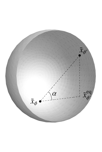
Figure 1: The vertical plane containing ${\bf\tilde{x}_{\phi}}$, ${\bf\tilde{x}_{\phi^{\prime}}}$.

This result has some analogy with the spectral distance computed on ${\cal P}(M_{2}({\mathbb{C}}))$ in [26], namely the rotation around the $z$-axis is an isometry and the distance on a parallel (${z_{\Psi}}={z_{\Psi^{\prime}}}$) is proportional to the Euclidean distance within the disk. But remarkably, while the distance on a meridian was infinite in [26], it remains finite here. This allows an easy “classical geometry” interpretation of Prop. 4.4. Assuming for convenience that $\tilde{z}_{\phi}\geq\tilde{z}_{\phi^{\prime}}$, let us call ${\bf\tilde{x}_{\phi^{\prime}}}^{eq}$ the projection of ${\bf\tilde{x}_{\phi^{\prime}}}$ in the $\tilde{z}_{\phi^{\prime}}$ plane and $\alpha$ the angle $({\bf\tilde{x}_{\phi}}{\bf\tilde{x}_{\phi^{\prime}}}^{eq},{\bf\tilde{x}_{\phi}}{\bf\tilde{x}_{\phi^{\prime}}})$ (see figure 1). Then

$$d(\omega_{\phi},\omega_{\phi^{\prime}})=\sqrt{\frac{\theta}{2}}\times\begin{cases}\cos\alpha\;\,d_{Ec}({\bf\tilde{x}_{\phi}},{\bf\tilde{x}_{\phi^{\prime}}})&\mathrm{when}\;\,\alpha\leq\frac{\pi}{4},\\ \frac{1}{2\sin\alpha}\,d_{Ec}({\bf\tilde{x}_{\phi}},{\bf\tilde{x}_{\phi^{\prime}}})&\mathrm{when}\;\,\alpha\geq\frac{\pi}{4}.\end{cases}$$

Note that by (4.13) this result is in agreement with (4.11). Also, two states with same $\tilde{x},\tilde{y}$ coordinates are at distance $\sqrt{\frac{\theta}{2}}\frac{\lvert\tilde{z}_{\phi}-\tilde{z}_{\phi^{\prime}}\rvert}{2}$. In particular the distance between the two poles — identified as $\omega_{0},\omega_{1}$ — is $\sqrt{\frac{\theta}{2}}$, in agreement with Proposition 3.6.

5 Conclusion

Describing the Moyal plane by a spectral triple based on the algebra of Schwartz functions equipped with Moyal $\star$-product (2.1), we have computed the spectral distance between the eigenfunctions of the quantum harmonic oscillator. We have shown that the distance is not finite on the whole of the pure-state space of $\mathcal{A}$, and that it can be made finite by truncating the Moyal spectral triple.

All the results in this paper are expressed in the matrix basis. It would be interesting to study the interpretation in the $x$-space. Can one see the pure states $\omega_{n}$ as deformation of some states of $C_{0}({\mathbb{R}}^{2})$? A relevant tool on that matter could be the coherent states of the harmonic oscillator.

The limit $\theta\rightarrow 0$ also deserves more attention. The pure state space for $\theta\neq 0$ (infinitely many pure states yielding the same representation modulo unitaries) is very different from the pure state space at $\theta=0$ (infinitely many pure states, the points of ${\mathbb{R}}^{2}$, yielding non-equivalent representations). This question should be addressed by using the continuous field of $C^{*}$-algebras, $\theta\mapsto\mathcal{A}_{\theta}=\overline{({\mathcal{S}},\star_{\theta})}$ where $\star_{\theta}$ is the Moyal product for the given value of the parameter.

One should also question the unitization problem. What is gained, from the metric point of view, by passing to the preferred unitization $\mathcal{A}_{1}$? In the commutative case, the algebra $C_{b}(X)$ of bounded continuous functions on a locally compact space $X$ is the maximal unitization of $C_{0}(X)$, and ${\cal P}(C_{b}(X))$ is the Stone-Čech compactification of ${\cal P}(C_{0}(X))\simeq X$. This is no longer true in the non-commutative case. In particular $\mathcal{A}_{1}$ is not the maximal unitization of $\mathcal{A}$ (which is the Moyal multiplier algebra ${\cal M}$). The link between ${\cal P}(\mathcal{A})$ and ${\cal P}(\mathcal{A}_{1})$ deserves further studies.

Finally, in the commutative case $\mathcal{A}=C_{0}^{\infty}(M)$, for $M$ a complete locally compact Riemannian manifold, the spectral distance between non-pure states coincides with the Wasserstein distance of order $1$ between probability distributions on $M$ [16]. Is there any possibility to associate a Wasserstein distance to the spectral distance on $S^{2}$ computed here?

Acknowledgements

The authors thank the anonymous referee for carefully reading the original manuscript and for many valuable remarks and suggestions. This work was partially supported by the ERG fellowship 237927 from the Europen Union.

References

• [1] E.M. Alfsen, Compact convex sets and boundary integrals, Springer-Verlag, Berlin, N.-Y., 1971.
• [2] G. Amelino-Camelia, G. Gubitosi, F. Mercati, Discreteness of area in noncommutative space, Phys.Lett. B676 (2009), 180–183.
• [3] D. Bahns, S. Doplicher, K. Fredenhagen, G. Piacitelli, Quantum geometry on quantum spacetime: distance, area and volume operators, arXiv: 1005.2130 [hep-th].
• [4] B. Blackadar. Operator algebras. Theory of $C^{*}$-algebras and von Neumann algebras. Encyclopaedia of Mathematical Sciences 122, 2006.
• [5] J.V. Bellissard, M. Marcolli, K. Reihani, Dynamical systems on spectral metric spaces, (2010), arXiv:1008.4617 [math.OA].
• [6] G. Bimonte, F. Lizzi, G. Sparano, Distances on a Lattice from Non-commutative Geometry, Phys.Lett. B341 (1994), 139–146
• [7] O. Bratteli, D.W. Robinson, Operator Algebras and Quant. Stat. Mech. 1, Springer Verlag, 1996.
• [8] E. Cagnache, T. Masson, J.C. Wallet, Noncommutative Yang-Mills-Higgs actions from derivation based differential calculus, J. Noncommut. Geom. 5 (2011), 39–67.
• [9] A. Connes, Noncommutative Geometry, Academic Press, 1994.
• [10] A. Connes, Noncommutative geometry and reality, J. Math. Phys. 36 (1995) 6194–6231.
• [11] A. Connes, On the spectral characterization of manifolds, arXiv:0810.2088 [math.OA].
• [12] A. Connes, M. Dubois-Violette, Noncommutative finite-dimensional manifolds I. spherical manifolds and related examples, Commun. Math. Phys. 230 (2002), 539–579.
• [13] A. Connes, G. Landi, Noncommutative manifolds: the instanton algebra and isospectral deformations, Commun. Math. Phys. 221 (2001), 141–159.
• [14] A. Connes, J. Lott, The metric aspect of noncommutative geometry, New symmetry principles in quantum field theory (Carg se 1991), p. 53-93, NATO Ad. Sci. Inst. Ser. B Phys. 295 Plenum, New York (1992).
• [15] E. Christensen, C. Ivan, Spectral triples for AF C*-algebras and metrics on the Cantor set, J. Operator Theory 56:1 (2006), 17–46.
• [16] F. D’Andrea, P. Martinetti, A view on optimal transport from noncommutative geometry, SIGMA 6 (2010), 057.
• [17] V.G. Drinfeld, Quantum groups, Proc. of the ICM, Berkeley 1 (1986), 798–820.
• [18] V. Gayral, B. Iochum, The spectral action for Moyal planes, J. Math. Phys. 46 (2005), 043503 .
• [19] V. Gayral, J.M. Gracia-Bondía, B. Iochum, T. Schücker, J.C. Várilly, Moyal planes are spectral triples, Commun. Math. Phys. 246 (2004), 569–623.
• [20] A. de Goursac, J.C. Wallet, R. Wulkenhaar, Noncommutative induced gauge theory, Eur. Phys. J. C. Part.Fields. 51 (2007), 977–987.
• [21] J.M. Gracia-Bondía, J.C. Várilly, Algebras of distributions suitable for phase-space quantum mechanics. I, J. Math. Phys., 29(4) (1988), 869–879.
• [22] J.M. Gracia-Bondía, J.C. Várilly, Algebras of distributions suitable for phase-space quantum mechanics. II, J. Math. Phys. 29(4) (1988), 880–887.
• [23] H.J. Groenewold, On the Principles of elementary quantum mechanics, Physica 12 (1946), 405–460.
• [24] H. Grosse, R. Wulkenhaar, Renormalisation of $\varphi^{4}$-theory on noncommutative $\mathbb{R}^{4}$ in the matrix basis, Commun. Math. Phys. 256 (2005), 305–374.
• [25] B. Iochum, T. Schücker, C. Stephan, On a Classification of Irreducible Almost Commutative Geometries, J. Math. Phys. 45 (2004), 5003–5041.
• [26] B. Iochum, T. Krajewski, P. Martinetti, Distances in Finite Spaces from Noncommutative Geometry, J. Geom. Phys. 37 (2001), no. 1-2, 100–125.
• [27] M. Jimbo, A $q$-difference analogue of $U(\mathfrak{g})$ and the Yang-Baxter equation, Lett. Math. Phys. 10 (1985), 63–69.
• [28] R.V. Kadison, J. R. Ringrose, Fundamentals of the theory of operators algebras II, Academic Press, 1986.
• [29] R.V. Kadison, A representation theory for commutative topological algebra, Mem. Amer. Math. Soc. 7 (1951).
• [30] D. Kaschek, N. Neumaier, S. Waldmann, Complete positivity of Rieffel’s deformation quantization by actions of $\mathbb{R}^{d}$, Jour. Noncommutative Geo. 3 (2009), 361–375.
• [31] F. Latrémolière, Bounded-Lipschitz distances on the state space of a $C^{*}$-algebra, Taiwanese J. Math. 11 (2007), no. 2, 447–469.
• [32] J. Madore, Fuzzy space-time, Can. J. Phys./Rev. can. phys. 75 6 (1997), 385–399.
• [33] P. Martinetti, Spectral distance on the circle, J. Func. Anal. 255 (2008), 1575–1612.
• [34] P. Martinetti, Carnot-Carathéodory metric from gauge fluctuation in noncommutative geometry, Comm. Math. Phys. 265 (2006), 585–616.
• [35] P. Martinetti, R. Wulkenhaar, Discrete Kaluza Klein from scalar fluctuations in non-commutative geometry, J. Math. Phys. 43 (2002), 182–204.
• [36] P. Martinetti, F. Mercati, L. Tomassini, Minimal length in quantum space and integrations of the line element in noncommutative geometry, arXiv: 1106.0261 [math-ph]
• [37] J.E. Moyal, Quantum mechanics as a statistical theory, Proc. Camb. Phil. Soc. 45 (1949), 99–124.
• [38] M.A. Rieffel, Deformation Quantization for Actions of $\mathbb{R}^{d}$, Memoirs of the Amer. Math. Soc. 506, Providence, RI, 1993.
• [39] M.A. Rieffel, Metric on state spaces, Documenta Math. 4 (1999), 559–600.
• [40] M.A. Rieffel, Compact quantum metric spaces, in “Operator algebras, quantization, and noncommutative geometry”, pp. 315–330, Contemp. Math. 365 (AMS, Providence, RI, 2004).
• [41] M.A. Rieffel, Gromov-Hausdorff distance for quantum metric spaces. Matrix algebras converge to the sphere for quantum Gromov-Hausdorff distance, Mem. AMS 168 (2004), no. 796, 1–65.
• [42] V. Rivasseau, F. Vignes-Tourneret, R. Wulkenhaar, Renormalization of noncommutative phi 4-theory by multi-scale analysis, Commun.Math.Phys. 262 (2006), 565–594.
• [43] C. Villani, Optimal Transport: Old and New, Springer, 2009.
• [44] J.C. Wallet, Derivations of the Moyal algebra and Noncommutative gauge theories, SIGMA 5 (2009) 013.