Close packing density of polydisperse hard spheres

Abstract

The most efficient way to pack equally sized spheres isotropically in 3D is known as the random close packed state, which provides a starting point for many approximations in physics and engineering. However, the particle size distribution of a real granular material is never monodisperse. Here we present a simple but accurate approximation for the random close packing density of hard spheres of any size distribution, based upon a mapping onto a one-dimensional problem. To test this theory we performed extensive simulations for mixtures of elastic spheres with hydrodynamic friction. The simulations show a general (but weak) dependence of the final (essentially hard sphere) packing density on fluid viscosity and on particle size, but this can be eliminated by choosing a specific relation between mass and particle size, making the random close packed volume fraction well-defined. Our theory agrees well with the simulations for bidisperse, tridisperse and log-normal distributions, and correctly reproduces the exact limits for large size ratios.

I Introduction

Granular materials such as sediments and powders are widespread in nature and industrial contexts, and treating the grains as hard spheres is often a useful first approximation. In these systems, the manner in which the grains pack together has profound influence on properties. Of these, random close packing1 is most likely to be encountered in tapped and consolidated systems, although other possibilities, such as random loose packing2 , and various crystalline arrangements (whose existence is very sensitive to the form of the size distribution and method of creation3 ; 4 ) are also possible.

Even though the precise nature (and for monodisperse spheres, even the existence5 ) of the random close packed state remains the subject of ongoing research6 , it provides a starting point for many approximations in both physics7 ; 8 and engineering, and has great practical importance not only for the prediction of the density of granular materials, but also other properties. For example, the viscosity of dense dispersions will diverge at this point9 and it is related to the permeability in packed beds10 .

One of the insights that have come forward from simulations6 is that the dense random packing density of hard spheres depends upon the (shear) friction coefficient, if the particles only lose energy by inelastic collisions. Further, the jamming density of a hard sphere system depends upon the initial state, and on the particular pathway chosen to cool down the system. In general, however, dissipative interactions play a role not just at contact. Granular particles suspended in a viscous medium also dissipate energy via long-range hydrodynamic interactions. Hence we anticipate that the dense random packing also depends upon solvent viscosity and on the range of the (hydrodynamic) friction. This is the first problem that we wish to address. To this end we developed a new simulation method that includes these effects. Using this method we not only find that the dense random packing depends on fluid viscosity, but – quite unexpectedly – also on particle size and mass. By analysing the various time scales in the problem we obtain a way to eliminate this dependence, which sheds new light upon the nature of the dense random packed state.

In practical cases the particle size distribution of a real granular material, or mixture of materials, is never monodisperse. Also for such polydisperse problems modelling techniques11 ; 12 have been used to calculate maximum packing fractions of spheres with a distribution of sizes. A typical example of a polydisperse system in a close packed state is shown in Fig. 1.

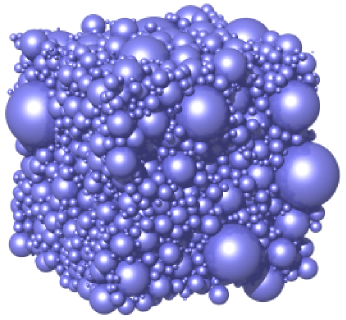
Figure 1: Close packed configuration of spheres from a log-normal distribution. The spread in the logarithm of radius is $\sigma=0.6$. Only spheres with centres lying in one periodic image of the simulation cell are shown.

The second problem that we wish to address is that these simulation methods are quite time consuming, and therefore their applicability is limited. It would be desirable to have an analytic expression for the close packing density, or a fast approximation, but progress in this direction has not been rapid. Ouchiyama and Tanaka13 have presented a theory based upon the volume occupied by a sphere in contact with other spheres of the mean diameter, but their results are at best qualitative, and the reasoning behind the method is not simple enough to suggest obvious improvements. Song et al.6 presented a theory for the packing of monodisperse spheres, but the generalisation to an arbitrary size distribution is not obvious. Recently Biazzo et al.14 presented a theory for binary mixtures, but like the Ouchiyama-Tanaka theory, it violates the exact upper limit for large fractions of big spheres that is given in Eq. (3) below. Thus, a comprehensive theory to predict the random close packing density of an arbitrary sphere mixture is still lacking.

We formulate such a theory, which is presented here in Section II. Next, we define our simulation method in Section III, and we present the combined theoretical and simulation results in Section IV. Conclusions are formulated in Section V.

II Theory

Here we propose an approximate solution to the problem of polydisperse packing density, obtained by abstracting what we believe to be essential features of the physics and geometry of packing. The fundamental problem we wish to solve is as follows: suppose we have a normalised distribution $P_{3D}(D)$ of sphere diameters defined so that $P_{3D}(D){\rm d}D$ equals the number fraction of spheres with diameters in the range $(D,D+{\rm d}D)$ present in the system. Then we ask what is the functional ${\cal F}:P_{3D}(D)\mapsto\phi_{\max}$ that maps the size distribution onto the random close packed volume fraction?

In order to construct this functional, we begin by mapping the 3D sphere packing problem onto a packing problem of rods in 1D. The corresponding 1D distribution $P_{1D}(L){\rm d}L$ gives the number fraction of rods with rod length in the range $(L,L+dL)$ present in the system. To do this we imagine a large random, but non-overlapping, arrangement of spheres in 3D with size distribution $P_{3D}(D)$. This need not be close packed for the argument that follows. Now imagine drawing a straight line through this distribution, and counting each portion of the line which lies within a sphere as a rod (see Fig. 2). The resulting distribution of rod lengths is then given by

$$P_{1D}(L)=2L\frac{\int_{L}^{\infty}P_{3D}(D){\rm d}D}{\int_{0}^{\infty}P_{3D}(D)D^{2}{\rm d}D}.$$ (1)

If rods of length $L_{i}$ are arranged on a line of length $\Lambda$ (with periodic boundary conditions), then the rod length fraction is clearly given by $\psi=\Lambda^{-1}\sum L_{i}$. This equals the volume fraction $\phi$ if there is a corresponding system of spheres in 3D.

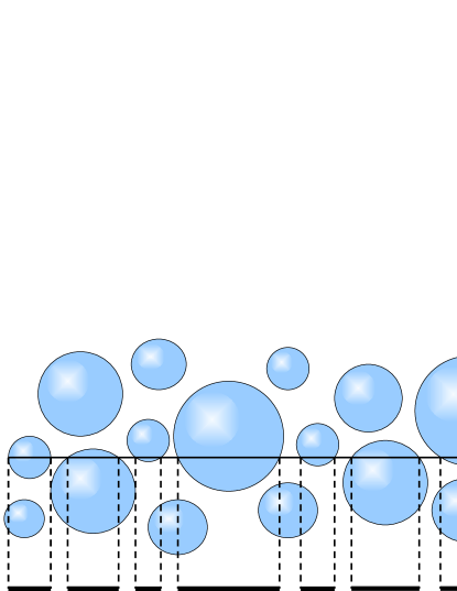
Figure 2: How to map a 3D sphere distribution onto a rod distribution. A straight line through a random arrangement of spheres defines a set of rods. The probability that a sphere is hit by the line is proportional to its cross sectional area and so proportional to $D^{2}P_{3D}(D)$. The probability that such a hit produces a rod of length $L$ is $2L/D^{2}$ (for $L<D$), and Eq. (1) in the text follows.

Let us assume that it is possible to map the closest random packing of spheres in 3D onto a problem of packing the above collection of rods on a line, where we search over all orderings of rods as well as their separations. This mapping will be achieved through an effective potential between the rods, which must have the following properties:

1. It should lead to a maximum packing fraction $\psi_{max}$ which is unchanged if all the rods (or spheres) are magnified by an equal amount;

2. The potential should be ‘hard’, in that it is either zero or infinite;

3. The interaction potential between large rods should reach through small rods. This will allow very small rods to ‘rattle around’ in the gaps between the large rods, so that at high weight fractions of large rods the latter can form a stress-bearing network;

4. The interaction range for mixtures of very unequal rods should be determined by the size of the smallest rod, so that small rods can form a dense randomly packed system in between the large rods, without leaving large gaps.

The true interaction potential between the rods will be both many-body and highly complicated, capturing topological aspects of 3D space. However, we suggest that the following pair potential is the simplest expression which honours the four requirements listed:

If two rods $i$ and $j$ have a gap $h$ between their nearest approaching ends, then we introduce the potential

$$V(h)=\left\{\begin{array}[]{lll}\infty&{\rm if}&h<\min(fL_{i},fL_{j})\\ 0&{\rm if}&h\geq\min(fL_{i},fL_{j})\end{array}\right.$$ (2)

where $f>0$ is a ‘free volume’ parameter. If this potential applies between any pair of rods, regardless of intervening rods in the gap between them, then it will satisfy requirement 3. The other requirements follow naturally. Rather than taking the minimum of the two lengths one could introduce a more complicated function of $L_{i}$ and $L_{j}$, but the present choice appears to be the simplest to capture the physics. In the remainder of this article $f$ will be used as a fit parameter; it is the only parameter in our theory, and can be chosen by requiring that the theory reproduces the random close packing of monodisperse systems.

For each ordering of the rods on the line, there is a shortest line which can accommodate them without incurring an infinite potential energy, and this leads to a close packing fraction for this ordering, which is simply $\psi=\Lambda^{-1}\sum L_{i}$. The maximum packing fraction $\psi_{\max}$ is the maximum value attained by $\psi$ over all possible orderings of the rods. If all the $L$’s are equal, $\psi_{\max}=(1+f)^{-1}$, and any rod polydispersity (which will always be present if we use Eq. (1)) will increase $\psi_{\max}$.

If we imagine inserting rods one at a time to form a packing, while increasing $\Lambda$ if necessary, then Eq. (2) constitutes a two-body potential between the inserted rod and all the rods currently in the packing. However, if rods are inserted in decreasing order of size, then the special choice of this potential means it only depends upon the newly inserted rod, and the packing further away is not disrupted by this process. To insert the new rod with a minimum increase of line length $\Lambda$ we need to identify the biggest gap. Therefore the following ‘greedy algorithm’15 may be used to find $\psi_{\max}$ for arbitrary $\{L_{i}\}$:

(a) The set of lengths $\{L_{i}\}$ is labelled such that $L_{1}\geq L_{2}\geq\ldots\geq L_{N}$. These will be inserted in decreasing order of lengths into the growing optimal packing, starting with $L_{1}$.

(b) Throughout the algorithm, we maintain a set of gaps $\{g_{i}\}$, equal in number to the number of rods we have inserted into the packing. At the start, when we have only one rod, this set contains one element $g_{1}=fL_{1}$.

(c) In order to insert rod $j$, we identify $g_{\max}$, the largest gap in the set of gaps, and we remove it from the set. We then add two new gaps to the set, namely $fL_{j}$ and $\max[g_{\max}-(1+f)L_{j},fL_{j}]$.

This process implicitly increases the line length $\Lambda$, if that is needed to accommodate the new rod.

Our final approximation consists of choosing a large number of rods from the distribution $P_{1D}(L)$, and packing them by the greedy 1D packing algorithm to obtain our estimate $\psi_{\max}$ for $\phi_{\max}$, the close packed volume fraction of the sphere distribution $P_{3D}$. Since this is essentially a sorting routine, the predictions of this algorithm take much less time (ca 0.3 seconds on a modern desktop computer) than explicit 3D simulation (1 to 30 hours). When the rod lengths are chosen at equidistant values of the cumulative 1D distribution, 2000 rods are sufficient for 5 decimal places accuracy. Thus, for $N$ rods we choose rod length $L_{i}$ such that $\int_{L_{i}}^{\infty}P_{1D}(l){\rm d}l=(N-i+1/2)/N$. We use $N=20000$ rods.

One useful property of this procedure is that it correctly reproduces the exact solution for bidisperse spheres with infinite size ratio. This limit is given by

$$\psi_{\max}=\min\left(\frac{\phi_{RCP}}{1-w(1-\phi_{RCP})},\frac{\phi_{RCP}}{w}\right),$$ (3)

where $\phi_{RCP}$ is the maximum packing fraction for a monodisperse system, and $w$ is the mass fraction of large spheres on the total particle volume, so $w=\phi_{\rm large}/(\phi_{\rm large}+\phi_{\rm small})$. Numerical solution of the theory for size ratios down to 1:1000 shows minor ($\sim 1\%$) deviations from the exact limit, for $w$ values very close to the cusp, $w=1/(2-\phi_{RCP})$.

The description above is complete, except that we need to specify the parameter $f$, which should be chosen such that the predicted maximum packing for monodisperse spheres is the correct random close packing value $\phi_{RCP}$. For monodisperse spheres we have $P_{1D}(L)=2LD_{0}^{-2}\theta(D_{0}-L)$ (where $\theta$ is the Heaviside step function), and we find that a value of $f=0.7654$ leads to a packing fraction of approximately $0.6435$. This value agrees with the simulation result described below, and is our only fit parameter.

III Simulation

Several methods have been proposed in the literature to simulate the dense random packing of hard spheres. One method used frequently was introduced by Lubachevsky and Stillinger,21 who simulated hard spheres by Molecular Dynamics and slowly compress the system until it jams. There is a drawback to this method, namely that ever smaller time steps need to be taken as close packing is approached. Moreover, the physical relaxation time of the system diverges near the close packing density,26 and consequently long runs are necessary. To circumvent this problem O’Hern et al.16 used soft spheres, and located the minimum energy by a conjugate gradient (CG) algorithm. This method is much faster than a hard sphere simulation, but the disadvantage is that the CG algorithm only simulates the high friction limit.

In general the dense random packing dependends on friction,6 and dissipative interactions may play a role not just at hard sphere contact. Granular particles suspended in a viscous medium also dissipate energy via long-range hydrodynamic interactions. Hence we anticipate that the dense random packing also depends upon solvent viscosity and on the range of friction. Therefore we introduce a new simulation method to include these effects.

Following O’Hern et al.16 and Groot and Stoyanov17 we simulate repulsive elastic spheres in the limit $T\rightarrow 0$. The generalization of the repulsive force in this model to elastic spheres of unequal size is

$$F_{ij}^{Rep}=2ER_{ij}(D_{ij}-r)\theta(D_{ij}-r).$$ (4)

Here, $r$ is the distance between particle centres, $D_{ij}=(D_{i}+D_{j})/2$ is the mean diameter and $R_{ij}$ is the harmonic mean radius given by $R_{ij}=\frac{1}{2}D_{i}D_{j}/D_{ij}$. The parameter $E$ is proportional to the linear elastic modulus of the particles17 . Henceforth we use $E=1000$.

Instead of using a CG algorithm to search the energy minimum, or imposing energy dissipation at particle collision, we introduce a soft friction function of finite range that represents the hydrodynamic interaction between spheres. A soft friction has been introduced before to simulate hydrodynamics in fluids, in the context of Dissipative Particle Dynamics27 ; 19 ; 20 . However, application to particles of unequal size is new to our knowledge, and because the dense random packing depends on friction some care must be taken in defining the friction function.

The most general distance-dependent friction is

$${\rm\bf F}_{ij}^{frict}=-\gamma_{ij}{\rm\bf v}_{ij}^{r}g(r/r_{c})$$ (5)

where $\gamma_{ij}$ is a friction factor that may depend on both particle sizes, ${\rm\bf v}_{ij}^{r}$ is the radial velocity difference, $g(r/r_{c})$ is a distance dependent function, and $r_{c}$ is a cut-off distance that may again depend on particle size.

Figure 3: Volume fraction obtained by extrapolating the $P-\phi$ curve to zero pressure.

To demonstrate the importance of the friction function, we first concentrate on monodisperse systems and study the influence of friction range and strength, and of particle size. We use a periodic $10\times 10\times 10$ box, containing from 1222 up to 1290 particles. All particles have diameter 1 and mass 1, and interact with a repulsive force $F=10^{3}(1-r)$ for $r<1$. First we study the influence of the range of the friction interaction. To this end we use the friction interaction ${\rm\bf F}_{ij}^{frict}=-{\rm\bf v}_{ij}^{r}(1-r/r_{c})^{2}/(1-1/r_{c})^{2}$; and the range is varied as $r_{c}=$ 1.5, 2, 3. With this choice for the friction force, the friction at particle contact is unity for all systems. All systems are evolved over $10^{4}$ steps or more, with $\delta t=0.01$. For each system the pressure at T = 0 was averaged over 5 independent starting configurations.

Even though all systems have the same friction strength at $r=1$, the mere range of friction appears to influence the pressure in the final state. As the friction range increases, so does the pressure at T = 0. In particular, the volume fraction to which the pressure extrapolates to zero – the dense random packing – varies systematically with the force range, see Fig. 3. Although the effect is not very large (about 1% variation), it is clear that the friction range does have an influence. The extrapolated value to $r_{c}=D=1$, $\phi_{cp}=0.6392\pm 0.0004$, compares well with the reported mean-field result for hard spheres with a friction interaction at contact,6 $\phi_{RCP}=0.634$. Thus we conclude that, to eliminate the influence of the friction range, the range must be scaled relative to the particle size.

Next, to demonstrate the influence of particle size and friction strength, a series of simulations was done where the ratio of the friction range relative to the particle diameter was kept fixed at $r_{c}/D$ = 1.5. The friction force used in this study was ${\rm\bf F}_{ij}^{frict}=-\gamma_{f}{\rm\bf v}_{ij}^{r}(1-r/r_{c})^{2}$, where $\gamma_{f}$ is a fixed friction factor, to be specified as input variable. Two sizes were studied, $D=1/2$ and $D=1$, and two friction factors were used, $\gamma_{f}=1$ and $\gamma_{f}=4$. In these simulations all particle masses were put at $m=1$. The box size was taken as $V=8^{3}$, and the conservative force was taken as $F=10^{3}D(D-r)$ for $r<D$, the same as in the previous simulations.

The results are shown in Fig. 4a. The red lines give the results of low viscosity ($\gamma_{f}=1$) and the black lines give the results of higher viscosity ($\gamma_{f}=4$). Results for small particles are denoted by open symbols and dashed curves, while results for big particles are denoted by closed symbols and full curves. This shows that both the friction factor and particle size influence the pressure in the glassy state. Consequently, the dense random packing density must depend on particle size. Even though the effect is small it is important, as it points at a reason why the dense random packing density is ill-defined. For practical reasons we wish to define a dense random packing density that does not depend on particle size, i.e. that is scale invariant. To obtain this, it is not sufficient to have a friction range that is proportional to the particle diameter; the packing density depends in a complicated way on particle size and on the strength and range of the friction force. Empirically there may seem to be some scaling when the friction is increased with the square of particle size (results for $D=1/2$, $\gamma_{f}=1$ in Fig. 4a partially overlap with $D=1$, $\gamma_{f}=4$), but the slopes of the curves are clearly different.

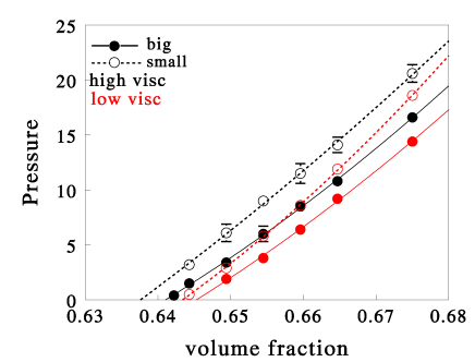
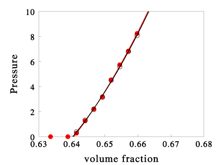
Figure 4: Mean pressure at T = 0 as function of particle volume fraction; a (top), for big particles (full symbols) and small particles (open symbols) and for low (red) and high (black) viscosity; b (bottom) big particles (red dots) and small particles (black circles) using friction as in Eq. (7) and mass $m=D$.

The above results show that we cannot just take any friction function. It must reflect the physical properties of the hydrodynamic interaction. One physical property is the scaling of the hydrodynamic force with particle size. On dimensional grounds the friction factor must be proportional to particle radius, as in Stokes’ law, $F=6\pi\eta av$. More generally, the (radial) squeeze mode of the hydrodynamic force between two rigid spheres at close contact behaves as18

$${\rm\bf F}_{ij}^{frict}=-\gamma{\rm\bf v}_{ij}^{r}R_{ij}g(h/R_{ij})\approx-\gamma{\rm\bf v}_{ij}^{r}\frac{R_{ij}^{2}}{h}$$ (6)

where $\gamma$ is the friction factor that is proportional to fluid viscosity, and $h=r-D_{ij}$ is the distance of closest approach. The function $g(x)\sim(1/x)$ is a scaling function that represents the lubrication force.

There is a large body of evidence showing that correct long-range inertial hydrodynamics is generated even if the (divergent) lubrication force between particles is replaced by a finite distance-dependent friction19 ; 20 . It is important however to choose the harmonic mean radius as the scaling length (unlike the conjecture by Kim and Karilla18 ), otherwise the friction between very unequal spheres would vanish if we remove the divergence of $g(x)$. Thus, we use the friction function

$${\rm\bf F}_{ij}^{frict}=-\gamma{\rm\bf v}_{ij}^{r}R_{ij}(1-h/R_{ij})^{2}\theta(R_{ij}-h).$$ (7)

which captures the right physics regarding the scaling of the range and strength of the viscous interaction with particle size.

Now we can turn to the problem of defining a size invariant dense random packing density. Therefore we analyse the relevant time scales of the problem. For a monodisperse system of elastic particles, a first time scale is the oscillation time, $t_{el}=2\pi(m/ED)^{1/2}$. This is the elastic time scale. The second time scale in the system is the drag relaxation time, $t_{d}=m/(\gamma D)$. The dense random packing can only be independent of particle size if we maintain a constant ratio between these two time scales, $t_{el}/t_{d}=2\pi\gamma(D/Em)^{1/2}$. Thus, we have scale invariance only if the friction factor satisfies $\gamma\propto(m/D)^{1/2}$. Since for most systems mass scales as $m\propto D^{3}$, this implies that for (soft) elastic spheres with hydrodynamic interaction the dense random packing fraction is (weakly) particle size dependent.

To obtain a well-defined dense random packing we are forced to choose the particle mass $m$ proportional to $D$. When this choice is made, the above ratio of time scales becomes particle size independent, and consequently the dense random packing fraction is well-defined. This choice has been made henceforth. The predicted scaling was checked by simulation and holds exactly. The pressure as function of time for systems of particle diameter $D=1/2$ and $D=1$ fall on top of each other if we scale the friction range with particle size (as in Eq. (7)) and simultaneously impose $m\propto D$. To demonstrate the improvement in system definition, two series of simulations were done, again for monodisperse systems of particle diameter $D=1/2$ and $D=1$, with repulsive force $F=10^{3}D(D-r)$ for $r<D$. For a realistic hydrodynamic scaling we used Eq. (7), with friction factor $\gamma=0.74$. Because the systems are monodisperse the cut-off distance for the friction interaction is $r_{c}=1.5D$, as in the previous case. To obtain scale invariance, we choose the masses as $m=D$. The systems had fixed volume $V=10^{3}$ for $D=1$ and $V=5^{3}$ for $D=1/2$. The systems were integrated over 5000 steps with time step $\delta t=0.01$ and the pressure was averaged over 10 independent runs. The comparison between small and big particles is shown in Fig. 4b. The predicted scaling is followed excellently.

Now that the system is well-defined, we can define a fast algorithm to obtain the close packing density. We use a variation of the Lubachevsky-Stillinger algorithm21 , where we make use of the relative softness of the interaction potential. We prepare the system in a random conformation (with particle overlaps) and then evolve it in an $(N,V,T)$ ensemble until we have a completely equilibrated state. For the parameters $\gamma=1$ and $\delta t=0.01$ that we used, this requires $3-50\times 10^{3}$ time steps. Then we switch to an $(N,P,T)$ ensemble, where the pressure is steered towards $P=0.01$, which is close enough in practice to $P=0$ (the error in $\phi_{\max}$ is of the order $10^{-5}$). If during a run the pressure falls below $0.001$ we switch to the L-S algorithm and compress the system in small steps until the pressure turns positive. The advantage of this method over the standard L-S algorithm is that the (high) pressure in the initial $(N,V,T)$ simulation quickly drives the system towards $P=0$. The final $(N,P,T)$ simulation serves to run down the $P-\phi$ curve (see Fig. 4b) to locate the intercept at $P=0$. Some minor evolution can however still be observed at $P=0.01$. To gain further simulation speed we combined a linked cell neighbour search with a Verlet neighbour list22 . In the late stages of evolution, when particles hardly move, this leads to a large increase in simulation speed, particularly for systems of large particle size difference.

Figure 5: a (top): Close packing density as function of the friction factor $\gamma$. Each data point is an average over 10 independent runs; b (bottom) same data, plotted to $1/\sqrt{\gamma}$.

Even though the close packing density is now well-defined, it still depends on friction, or the cooling rate, see Fig. 5. In fact this is the very source of the previously found dependence of the close packing density on particle size and mass. To study this relation, monodisperse systems of 6000 particles were used. All particles have diameter 1 and mass 1, and interact with a repulsive force with $E=10^{3}$. We insert the particles in a box of size $16.83$ (or $\phi=0.66$), pre-equilibrate for $5\times 10^{4}$ to $2\times 10^{5}$ time steps of $\delta t=0.01$ until the pressure has fully equilibrated. Then we run a constant pressure ensemble, steering the pressure to $P=0.01$, until the volume fraction is stable over four decimal places ($1.5\times 10^{5}$ time steps). All results are averaged over 10 runs. Polycrystalline domains only start to occur for $\gamma<0.03$; all systems shown here are isotropic. Over about a decade we find a $\log(\gamma)$ dependence for $\gamma\rightarrow 0$ (see Fig. 5a), and over two decades we find a power law decay $\phi\approx 0.64+0.0028/\sqrt{\gamma}$ for $\gamma>1/4$ (see Fig. 5b). Therefore we have to make a choice for the friction factor, and only refer to the packing fraction at that value of $\gamma$. Our default value used in the next section is $\gamma=1$.

For comparison we also evolved a system from its initial conformation to equilibrium using a steepest descent method in an $(N,V,T)$ ensemble, which should compare well with the CG algorithm16 . The final pressure coincides with our result at $\gamma\rightarrow\infty$, which demonstrates that CG simulates the high viscosity limit. For truly hard spheres the modulus diverges, hence the ratio $t_{el}/t_{d}=2\pi\gamma(D/Em)^{1/2}\rightarrow 0$. To simulate this with particles of finite modulus, low values of $\gamma$ would be preferred. This implies that the present method is closer to the physical case than the CG algorithm to generate hard spheres conformations, unless largely inelastic collisions are pertinent.

IV Results

The simple approximation for ${\cal F}$ described in section II is now compared with the results from the sphere packing simulation method of section III. Consider first bidisperse spheres, as studied for example by Clarke and Wiley23 and by Yerazunis et al.24 , where the larger spheres have $R$ times the radius of the smaller, so that $P_{3D}(D)\propto R^{3}(1-w)\delta(D-1/R)+w\delta(D-1)$. The simulation results for binary mixtures are shown in Table 1, and in Fig. 6, together with the theoretical prediction. The big particles have diameter $D_{1}=$ 1, and the small particle diameters are $D_{2}=$ 0.5, 0.3, 0.2 and 0.1. The dash-dot curve gives the exact upper limit of the volume fraction, Eq. (3). For diameter $D_{2}\geq 0.2$ we used $6000$ particles; for $D_{2}=0.1$ we used up to $N=49950$ particles (at $w=0.8$) to prevent finite size effects. All runs were evolved over a minimum of 150 000 time steps, and convergence of the volume fraction was checked by extending the evolution of selected systems to 450 000 steps. All volume fraction results shown in Fig. 6 are stable up to four decimal places.

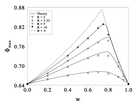
Figure 6: Maximum packing fraction for bidisperse spheres of different size. $R$ is the size ratio, and $w=\phi_{\rm large}/(\phi_{\rm large}+\phi_{\rm small})$ is the relative volume fraction of the large spheres. Symbols are simulation results, and solid lines are theoretical predictions, based on 20000 rods. The dashed curves give the upper limit for infinite size ratio, Eq. (3).

Table 1: Simulation results for the maximum packing fraction of bidisperse sphers, with diameters $D_{1}$ and $D_{2}$. The mass fraction present in the large spheres is given by $w=\phi_{\rm large}/(\phi_{\rm large}+\phi_{\rm small})$.

$w$	$D_{2}/D_{1}=0.5$	$D_{2}/D_{1}=0.3$	$D_{2}/D_{1}=0.2$	$D_{2}/D_{1}=0.1$
0	0.6435	0.6435	0.6435	0.6435
0.2	0.6579	0.6695	0.6761
0.4	0.6690	0.6971	0.7152	0.7298
0.5				0.7557
0.6	0.6774	0.7236	0.7525	0.7835
0.7	0.6795	0.7324	0.7714	0.8150
0.75				0.8270
0.8	0.6749	0.7315	0.7769	0.7948
0.9	0.6650	0.6985	0.7111
0.95	0.6558	0.6690
1	0.6435	0.6435	0.6435	0.6435

A bidisperse system, with moderate to large size ratios, has two distinct regimes (and a non-trivial crossover between them): When the proportion of large spheres is low, they are isolated from one another, like holes in a Swiss cheese; while the small spheres form a close-packed phase (the ‘cheese’) between them. On the other hand, when the proportion of large spheres is high, these form a close-packed structure, leaving the small spheres to ‘rattle around’ in the gaps between them. Recent theories of the close packed state of bidisperse spheres14 ; 25 do not address the ‘rattler’ regime adequately. In contrast, our theory captures both regimes (exactly, in the limit of infinite size ratio), and also the analogous regimes which are produced for larger numbers of size classes, such as tridiperse spheres.

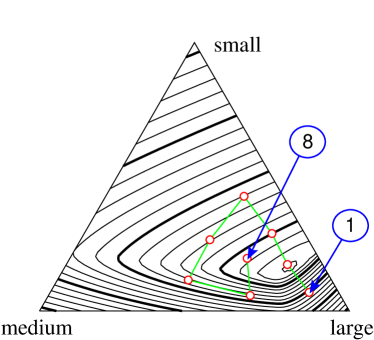
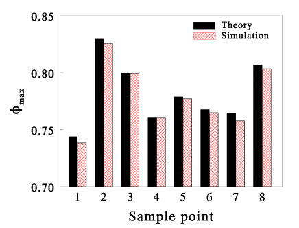
Figure 7: Maximum packing fraction for a tridisperse distribution of spheres with size ratios 1:3:9. The composition diagram (a, top) is based on weight fractions; contour lines connect points of equal volume fraction, with bold lines at volume fractions of 0.65, 0.7, 0.75 and 0.8. The compositions used in the simulations are marked by the circles; b (bottom) shows the comparison between theory and simulation per sample point.

Next, we consider a tridisperse distribution. In particular we consider the case where the sphere diameters are in the ratio 1:3:9. Fig. 7 shows the theoretical prediction compared with simulation results for selected points. The number of particles chosen varies from 6000 to 13400. Particular care was taken at large weight fractions of big particles, where these may form a stress bearing network. A finite size study showed that in that case (specifically sample point 1) the number of large particles in the system needs to be above 175 for reliable results. For sample point 1 we used 209 big particles from a total of 13300. Again, the theory compares very well with the simulation results. The differences may well be attributed to remaining (minor) finite size effects.

Figure 8: Maximum packing fraction for a log-normal distribution. The spread in log(radius) is denoted by $\sigma$. Simulation results are given by symbols; the solid line is the theoretical prediction, based on 20000 rods.

Finally, we consider a log-normal distribution, which is defined as $P_{3D}(D)\propto\exp(-[\ln(D/D_{0})]^{2}/2\sigma^{2})/D$. Thus, from Eq. (2), we find the rod distribution in the theory as $P_{1D}(L)\propto L\ {\rm erfc}[\ln(L/D_{0})/\sigma\sqrt{2}]$. In these simulations we set an upper diameter to the particles $D=1$, and choose the mean diameter such that less than 0.1% of the particles exceed this size. We used 6000 particles that were evolved over 50 000 to 200 000 steps, until the volume fraction had converged up to 4 decimal places. Fig. 8 shows the comparison between theory and simulation data. The system at $\sigma=0.6$ is shown in Fig. 1. Again, the theory compares very well with the simulation results.

V Conclusions

Concluding, we have introduced a theory for the close packing density of hard spheres of arbitrary size distribution, based on a mapping onto a one-dimensional problem. To test the theory we simulated the dense random packing of (soft) elastic spheres with hydrodynamic friction in 3D in the limit $T\rightarrow 0$, which approaches the hard sphere system. For the distributions studied we obtain excellent agreement between theory and simulation. The theory reproduces the infinite size ratio limit for bidisperse spheres. Hence we expect that this approximation will prove useful for more general size distributions. The simple structure of the approximation may also be amenable to further analysis, and open up new avenues for analytical approximations.

Application of this theory to other space dimensions than 3D is straightforward. However, a comparison between theory and simulations showed that, although the theory is qualitatively correct in 2D, it does not reproduce the simulations as accurately as in 3D. This may be related to the mean-field character of the theory, i.e. the explicit spatial correlation is lost in the theory. We therefore speculate that the theory will be accurate in 3D and in higher dimensions.

The simulations show a weak dependence of the dense random packing on fluid viscosity, if the friction force is of hydrodynamic origin. In general the dense random packing density also depends on particle size, mass and elastic modulus. For particles of diameter $D$, mass $m$ and elastic modulus $E$, suspended in a liquid of viscosity $\eta$, we infer that the dense random packing density should be a function of the dimensionless group $Q=\eta^{2}D/(Em)$. For systems of the same $Q$ value but different size, mass and viscosity we find excellent scaling of the pressure as function of time. Therefore we conclude that the size dependence of dense random packing is a kinetic effect that disappears when $m\propto D$. Although such scaling is artificial, it leads to a well-defined dense random packing, which is prudent to test theories that are based only on geometrical considerations.

References

- (1) J. Bernal, J. Mason, Nature 188, 910 (1960).
- (2) G. Y. Onoda, E. G. Liniger, Phys. Rev. Lett. 64, 2727 (1990).
- (3) A. Imhof, J. K. G. Dhont, Phys. Rev. Lett. 75(8), 1622 (1995).
- (4) K. P. Velikov, C. G. Christova, R. P. A. Dullens, A. van Blaaderen, Science 296, 106 (2002).
- (5) S. Torquato, T. M. Truskett, P. G. Debenedetti, Phys. Rev. Lett. 84, 2064 (2000).
- (6) C. Song, P. Wang, H. A. Makse, Nature 453, 629 (2008).
- (7) P. G. Debenedetti, F. H. Stillinger, Nature 410, 259 (2001).
- (8) H. M. Jaeger, S. R. Nagel, R. P. Behringer, Rev. Mod. Phys. 68, 1259 (1996).
- (9) I. M. Krieger, Adv. Col. Int. Sci. 3, 111 (1972).
- (10) R. J. Hill, D. L. Koch, A. J. C. Ladd, J. Fluid Mech. 448, 243 (2001).
- (11) S. E. Phan, W. B. Russel, J. X. Zhu, P. M. Chaikin, J. Chem. Phys. 108, 9789 (1998).
- (12) A. R. Kansal, S. Torquato, F. H. Stillinger, J. Chem. Phys. 117, 8212 (2002).
- (13) N. Ouchiyama, T. Tanaka, Ind. Eng. Chem. Fundam. 20, 66 (1981).
- (14) I. Biazzo, F. Caltagirone, G. Parisi, F. Zamponi, Phys. Rev. Lett. 102, 195701 (2009).
- (15) T. H. Cormen, C. E. Leiserson, R. L. Rivest, C Stein, C., Introduction to Algorithms (MIT Press, Cambridge, Mass., 2003).
- (16) B. D. Lubachevsky, F. H. Stillinger, J. Stat. Phys. 60, 561 (1990).
- (17) M. Hermes and M. Dijkstra, Random close packing of polydisperse hard spheres, http://arXiv.org/abs/0903.4075v1 (2009).
- (18) C. S. O’Hern, S. A. Langer, A. J. Liu, S. R. Nagel, Phys. Rev. Lett. 88, 075507 (2002).
- (19) R. D. Groot, S. D. Stoyanov, Phys. Rev. E 78, 051403 (2008).
- (20) P. J. Hoogerbrugge and J. M. V. A. Koelman, Europhys. Lett. 19, 155 (1992).
- (21) P. Espanol, Phys. Rev. E 52, 1734 (1995).
- (22) R. D. Groot, P. B. Warren, J. Chem. Phys. 107, 4423 (1997).
- (23) S. Kim, L. Karilla, Microhydrodynamics: Principles and Selected Applications (Butterworth-Heinemann, Stoneham, MA, 1991).
- (24) M. P. Allen, D. J. Tildesley, Computer simulation of liquids (Clarendon Press, Oxford, 1987).
- (25) A. S. Clarke, J. D. Wiley, Phys. Rev. B 35, 7350 (1987).
- (26) S. Yerazunis, S. W. Cornell, B. Wintner, Nature 207, 835 (1965).
- (27) M. Clusel, E. I. Corwin, A. O. N. Siemens, J. Brujic, Nature 460, 611 (2009).